class: center, middle, inverse, title-slide .title[ # CS&SS 569 Visualizing Data and Models ] .subtitle[ ## Lab 6: Visualizing spatial data ] .author[ ### Ramses Llobet ] .institute[ ### Department of Political Science, UW ] .date[ ### 2025-02-14 ] --- ## Introduction - A long rant on space: What do we mean when we say visualizing "spatial data"? -- 1. Physical world - Physical, spatial features: geographical area, features, contours, etc -- 2. Social world - Some socio-economic-political variables that could be mapped onto physical, geographical features - E.g., district-level income level, crime rate, education spending, etc -- 3. Graphical space as dimension(s) to express some variables - E.g., x and y coordinates on our 2D canvas --- ## Introduction - We can project (1) physical space onto (3) graphical space - Traditional understanding of "map" -- - We can project (2) social variables directly onto (3) graphical space - Bubble plot uses size/area to express magnitude; bar plot uses length to express magnitude -- - Problems start to occur when we project (2) social variables onto (1) physical space, then onto (3) graphical space - Let's say we want to visualize some district-level covariates -- - Problem 1: incongruity b/w social space and physical space - We visualize district-level variables onto the whole WA state; too much extrapolation -- - Problem 2: why do we prioritize physical space? - E.g., why a vast piece of land w/ little people should be prioritized over a small but densely populated area? - Can we use variables other than physical space to mediate (2) and (3)? --- ## (In)famous US election map... <img src="pictures/trumpMap.png" width="40%" style="display: block; margin: auto;" /> --- ## ... inspires many advances in visualizing spatial data <img src="pictures/election-maps-top-24-us-elections-2020-results-data-visualization-blog.png" width="52.5%" style="display: block; margin: auto;" /> --- ## But the problem is more common than you think... <img src="pictures/alaskaMaps.png" width="90%" style="display: block; margin: auto;" /> --- ## Popular ways to visualize spatial data: Choropleth map <img src="pictures/NYT_map1.png" width="45%" style="display: block; margin: auto;" /> --- ## Popular ways to visualize spatial data: Choropleth map w/ small multiples <img src="pictures/NYT_map2.png" width="35%" style="display: block; margin: auto;" /> --- ## Popular ways to visualize spatial data: Geo-faceted small multiples <img src="pictures/Economist_geofacet.png" width="37.5%" style="display: block; margin: auto;" /> --- ## Popular ways to visualize spatial data: Cartogram heatmap <img src="pictures/WA_statebins.png" width="90%" style="display: block; margin: auto;" /> --- ## Popular ways to visualize spatial data: Tiled cartogram <img src="pictures/tileCartogram.png" width="67.5%" style="display: block; margin: auto;" /> --- ## Roadmap - Cover different ways to visualize spatial data: -- - Geo-faceted small multiples w/ package **`geofacet`** -- - Cartogram heatmap w/ package **`statebins`** -- - Tiled cartogram w/ package **`tilegramsR`** -- - Choropleth maps (a.k.a. "maps'') -- - Brief introduction to spatial data file (e.g., shapefile; `.shp`) -- - package **`sf`** to wrangle spatial data and **`tmap`** to visualize map -- - Interactive maps; small multiples in choropleth maps -- - Be mindful of the issues of space(s) and the curse of dimensionality -- - How to incorporate time series or extra covariates when visualizing spatial data? --- ## Prerequisite ``` r # download packages packages <- c("tidyverse", "geofacet", "statebins", "tilegramsR", "sf", "tmap", "tigris") not_installed <- setdiff(packages, rownames(installed.packages())) if (length(not_installed)) install.packages(not_installed) # load packages library(tidyverse) library(geofacet) library(statebins) library(tilegramsR) library(sf) library(tmap) library(maptiles) library(tigris) # load theme source("https://students.washington.edu/kpleung/vis/theme_cavis.R") ``` --- count: false ## Geo-faceted small multiples .panel1-geofacet1-auto[ ``` r *WaPo_data <- read_csv("data/WaPo_data.csv") ``` ] .panel2-geofacet1-auto[ ] --- count: false ## Geo-faceted small multiples .panel1-geofacet1-auto[ ``` r WaPo_data <- read_csv("data/WaPo_data.csv") *print(WaPo_data, n = 5) ``` ] .panel2-geofacet1-auto[ ``` # A tibble: 51 × 23 stab state share_cut1994 share_cut1995 share_cut1996 share_cut1997 <chr> <chr> <dbl> <dbl> <dbl> <dbl> 1 NC North Carolina 1.4 0.9 3 4.1 2 AL Alabama 1.1 2.4 5.2 4.6 3 MS Mississippi 2 3.9 5.1 2.2 4 AR Arkansas 1.6 1.3 1.6 2.7 5 TN Tennessee 1.6 2 3.4 3.5 # ℹ 46 more rows # ℹ 17 more variables: share_cut1998 <dbl>, share_cut1999 <dbl>, # share_cut2000 <dbl>, share_cut2001 <dbl>, share_cut2002 <dbl>, # share_cut2003 <dbl>, share_cut2004 <dbl>, share_cut2005 <dbl>, # share_cut2006 <dbl>, share_cut2007 <dbl>, share_cut2008 <dbl>, # share_cut2009 <dbl>, share_cut2010 <dbl>, share_cut2011 <dbl>, # share_cut2012 <dbl>, share_cut2013 <dbl>, avgshare <dbl> ``` ] <style> .panel1-geofacet1-auto { color: black; width: 88.2%; hight: 32%; float: top; padding-left: 1%; font-size: 80% } .panel2-geofacet1-auto { color: black; width: 9.8%; hight: 32%; float: top; padding-left: 1%; font-size: 80% } .panel3-geofacet1-auto { color: black; width: NA%; hight: 33%; float: top; padding-left: 1%; font-size: 80% } </style> --- count: false ## Geo-faceted small multiples .panel1-geofacet2-auto[ ``` r # convert the data into long format *WaPo_data ``` ] .panel2-geofacet2-auto[ ``` # A tibble: 51 × 23 stab state share_cut1994 share_cut1995 share_cut1996 share_cut1997 <chr> <chr> <dbl> <dbl> <dbl> <dbl> 1 NC North Carolina 1.4 0.9 3 4.1 2 AL Alabama 1.1 2.4 5.2 4.6 3 MS Mississippi 2 3.9 5.1 2.2 4 AR Arkansas 1.6 1.3 1.6 2.7 5 TN Tennessee 1.6 2 3.4 3.5 6 SC South Carolina 1.5 1 2.5 0.7 7 ME Maine 2.3 1.9 3.5 1.7 8 MI Michigan 0.3 0.4 1.1 0.9 9 OR Oregon 0.4 0.7 1.3 0.8 10 KY Kentucky 2.5 1 3.1 1.8 # ℹ 41 more rows # ℹ 17 more variables: share_cut1998 <dbl>, share_cut1999 <dbl>, # share_cut2000 <dbl>, share_cut2001 <dbl>, share_cut2002 <dbl>, # share_cut2003 <dbl>, share_cut2004 <dbl>, share_cut2005 <dbl>, # share_cut2006 <dbl>, share_cut2007 <dbl>, share_cut2008 <dbl>, # share_cut2009 <dbl>, share_cut2010 <dbl>, share_cut2011 <dbl>, # share_cut2012 <dbl>, share_cut2013 <dbl>, avgshare <dbl> ``` ] --- count: false ## Geo-faceted small multiples .panel1-geofacet2-auto[ ``` r # convert the data into long format WaPo_data %>% * select(-avgshare) ``` ] .panel2-geofacet2-auto[ ``` # A tibble: 51 × 22 stab state share_cut1994 share_cut1995 share_cut1996 share_cut1997 <chr> <chr> <dbl> <dbl> <dbl> <dbl> 1 NC North Carolina 1.4 0.9 3 4.1 2 AL Alabama 1.1 2.4 5.2 4.6 3 MS Mississippi 2 3.9 5.1 2.2 4 AR Arkansas 1.6 1.3 1.6 2.7 5 TN Tennessee 1.6 2 3.4 3.5 6 SC South Carolina 1.5 1 2.5 0.7 7 ME Maine 2.3 1.9 3.5 1.7 8 MI Michigan 0.3 0.4 1.1 0.9 9 OR Oregon 0.4 0.7 1.3 0.8 10 KY Kentucky 2.5 1 3.1 1.8 # ℹ 41 more rows # ℹ 16 more variables: share_cut1998 <dbl>, share_cut1999 <dbl>, # share_cut2000 <dbl>, share_cut2001 <dbl>, share_cut2002 <dbl>, # share_cut2003 <dbl>, share_cut2004 <dbl>, share_cut2005 <dbl>, # share_cut2006 <dbl>, share_cut2007 <dbl>, share_cut2008 <dbl>, # share_cut2009 <dbl>, share_cut2010 <dbl>, share_cut2011 <dbl>, # share_cut2012 <dbl>, share_cut2013 <dbl> ``` ] --- count: false ## Geo-faceted small multiples .panel1-geofacet2-auto[ ``` r # convert the data into long format WaPo_data %>% select(-avgshare) %>% * pivot_longer(contains("share_cut"), names_to = "year", values_to = "share_cut") ``` ] .panel2-geofacet2-auto[ ``` # A tibble: 1,020 × 4 stab state year share_cut <chr> <chr> <chr> <dbl> 1 NC North Carolina share_cut1994 1.4 2 NC North Carolina share_cut1995 0.9 3 NC North Carolina share_cut1996 3 4 NC North Carolina share_cut1997 4.1 5 NC North Carolina share_cut1998 3 6 NC North Carolina share_cut1999 3.9 7 NC North Carolina share_cut2000 1.5 8 NC North Carolina share_cut2001 3.8 9 NC North Carolina share_cut2002 6.1 10 NC North Carolina share_cut2003 6.7 # ℹ 1,010 more rows ``` ] --- count: false ## Geo-faceted small multiples .panel1-geofacet2-auto[ ``` r # convert the data into long format WaPo_data %>% select(-avgshare) %>% pivot_longer(contains("share_cut"), names_to = "year", values_to = "share_cut") %>% * mutate(year = str_extract(year, "\\d+"), * year = as.numeric(year)) ``` ] .panel2-geofacet2-auto[ ``` # A tibble: 1,020 × 4 stab state year share_cut <chr> <chr> <dbl> <dbl> 1 NC North Carolina 1994 1.4 2 NC North Carolina 1995 0.9 3 NC North Carolina 1996 3 4 NC North Carolina 1997 4.1 5 NC North Carolina 1998 3 6 NC North Carolina 1999 3.9 7 NC North Carolina 2000 1.5 8 NC North Carolina 2001 3.8 9 NC North Carolina 2002 6.1 10 NC North Carolina 2003 6.7 # ℹ 1,010 more rows ``` ] --- count: false ## Geo-faceted small multiples .panel1-geofacet2-auto[ ``` r # convert the data into long format WaPo_data %>% select(-avgshare) %>% pivot_longer(contains("share_cut"), names_to = "year", values_to = "share_cut") %>% mutate(year = str_extract(year, "\\d+"), year = as.numeric(year)) -> * WaPo_data_long ``` ] .panel2-geofacet2-auto[ ] <style> .panel1-geofacet2-auto { color: black; width: 88.2%; hight: 32%; float: top; padding-left: 1%; font-size: 80% } .panel2-geofacet2-auto { color: black; width: 9.8%; hight: 32%; float: top; padding-left: 1%; font-size: 80% } .panel3-geofacet2-auto { color: black; width: NA%; hight: 33%; float: top; padding-left: 1%; font-size: 80% } </style> --- count: false ## Geo-faceted small multiples .panel1-geofacet3-auto[ ``` r *ggplot(WaPo_data_long, aes(x = year , y = share_cut)) ``` ] .panel2-geofacet3-auto[ <!-- --> ] --- count: false ## Geo-faceted small multiples .panel1-geofacet3-auto[ ``` r ggplot(WaPo_data_long, aes(x = year , y = share_cut)) + * theme_cavis_hgrid ``` ] .panel2-geofacet3-auto[ <!-- --> ] --- count: false ## Geo-faceted small multiples .panel1-geofacet3-auto[ ``` r ggplot(WaPo_data_long, aes(x = year , y = share_cut)) + theme_cavis_hgrid + * geom_line() ``` ] .panel2-geofacet3-auto[ <!-- --> ] --- count: false ## Geo-faceted small multiples .panel1-geofacet3-auto[ ``` r ggplot(WaPo_data_long, aes(x = year , y = share_cut)) + theme_cavis_hgrid + geom_line() + * facet_wrap(~ state) ``` ] .panel2-geofacet3-auto[ <!-- --> ] --- count: false ## Geo-faceted small multiples .panel1-geofacet3-auto[ ``` r ggplot(WaPo_data_long, aes(x = year , y = share_cut)) + theme_cavis_hgrid + geom_line() + facet_wrap(~ state) + * scale_x_continuous( * labels = function(x) paste0("'", str_sub(x, 3, 4)) * ) ``` ] .panel2-geofacet3-auto[ <!-- --> ] --- count: false ## Geo-faceted small multiples .panel1-geofacet3-auto[ ``` r ggplot(WaPo_data_long, aes(x = year , y = share_cut)) + theme_cavis_hgrid + geom_line() + facet_wrap(~ state) + scale_x_continuous( labels = function(x) paste0("'", str_sub(x, 3, 4)) ) + * scale_y_continuous( * labels = function(x) paste0(x, "%") * ) ``` ] .panel2-geofacet3-auto[ <!-- --> ] --- count: false ## Geo-faceted small multiples .panel1-geofacet3-auto[ ``` r ggplot(WaPo_data_long, aes(x = year , y = share_cut)) + theme_cavis_hgrid + geom_line() + facet_wrap(~ state) + scale_x_continuous( labels = function(x) paste0("'", str_sub(x, 3, 4)) ) + scale_y_continuous( labels = function(x) paste0(x, "%") ) + * theme( * strip.text.x = element_text(size = 7), * axis.text.x = element_text(size = 7), * axis.text.y = element_text(size = 7) * ) ``` ] .panel2-geofacet3-auto[ <!-- --> ] --- count: false ## Geo-faceted small multiples .panel1-geofacet3-auto[ ``` r ggplot(WaPo_data_long, aes(x = year , y = share_cut)) + theme_cavis_hgrid + geom_line() + facet_wrap(~ state) + scale_x_continuous( labels = function(x) paste0("'", str_sub(x, 3, 4)) ) + scale_y_continuous( labels = function(x) paste0(x, "%") ) + theme( strip.text.x = element_text(size = 7), axis.text.x = element_text(size = 7), axis.text.y = element_text(size = 7) ) + * labs(x = NULL, y = "Share of job loss due to trade") ``` ] .panel2-geofacet3-auto[ <!-- --> ] <style> .panel1-geofacet3-auto { color: black; width: 49%; hight: 32%; float: left; padding-left: 1%; font-size: 80% } .panel2-geofacet3-auto { color: black; width: 49%; hight: 32%; float: left; padding-left: 1%; font-size: 80% } .panel3-geofacet3-auto { color: black; width: NA%; hight: 33%; float: left; padding-left: 1%; font-size: 80% } </style> --- count: false ## Geo-faceted small multiples .panel1-geofacet3-rotate[ ``` r ggplot(WaPo_data_long, aes(x = year , y = share_cut)) + theme_cavis_hgrid + geom_line() + * facet_geo(~ state, grid = "us_state_grid2") + scale_x_continuous( labels = function(x) paste0("'", str_sub(x, 3, 4)) ) + scale_y_continuous( labels = function(x) paste0(x, "%") ) + theme( strip.text.x = element_text(size = 7), axis.text.x = element_text(size = 7), axis.text.y = element_text(size = 7) ) + labs(x = NULL, y = "Share of job loss due to trade") ``` ] .panel2-geofacet3-rotate[ 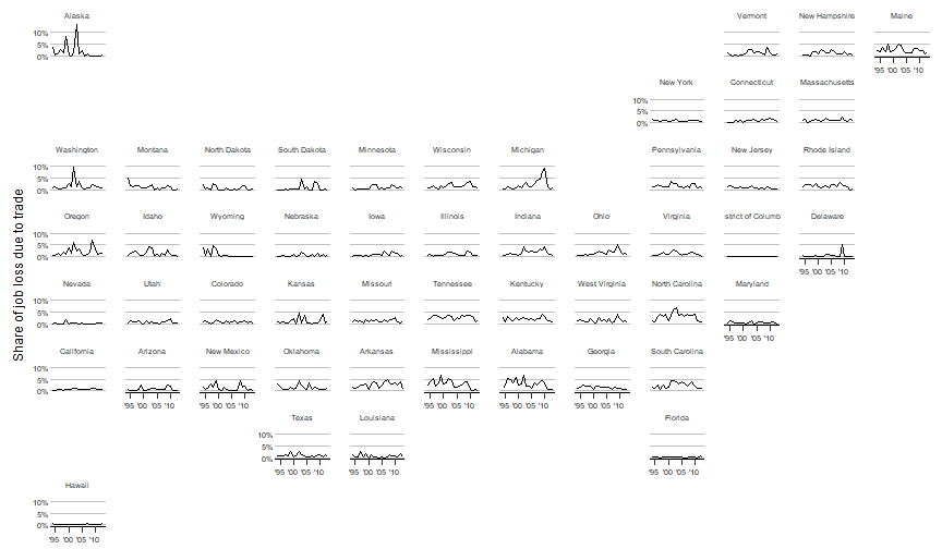<!-- --> ] --- count: false ## Geo-faceted small multiples .panel1-geofacet3-rotate[ ``` r ggplot(WaPo_data_long, aes(x = year , y = share_cut)) + theme_cavis_hgrid + geom_line() + * facet_geo(~ state, grid = "us_state_grid1") + scale_x_continuous( labels = function(x) paste0("'", str_sub(x, 3, 4)) ) + scale_y_continuous( labels = function(x) paste0(x, "%") ) + theme( strip.text.x = element_text(size = 7), axis.text.x = element_text(size = 7), axis.text.y = element_text(size = 7) ) + labs(x = NULL, y = "Share of job loss due to trade") ``` ] .panel2-geofacet3-rotate[ 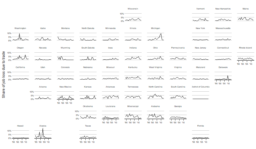<!-- --> ] <style> .panel1-geofacet3-rotate { color: black; width: 49%; hight: 32%; float: left; padding-left: 1%; font-size: 80% } .panel2-geofacet3-rotate { color: black; width: 49%; hight: 32%; float: left; padding-left: 1%; font-size: 80% } .panel3-geofacet3-rotate { color: black; width: NA%; hight: 33%; float: left; padding-left: 1%; font-size: 80% } </style> --- ## Geo-faceted small multiples - Check out the [available grids](https://hafen.github.io/geofacet/articles/geofacet.html) (users submitted) -- - You can build your own grid using [Geo Grid Designer](https://hafen.github.io/grid-designer/) and make it a public good --- ## Cartogram Heatmaps <img src="pictures/WA_statebins.png" width="75%" style="display: block; margin: auto;" /> --- count: false ## Cartogram heatmaps with statebins package .panel1-statebins1-auto[ ``` r # coerce avgshare into a factor *WaPo_data ``` ] .panel2-statebins1-auto[ ``` # A tibble: 51 × 23 stab state share_cut1994 share_cut1995 share_cut1996 share_cut1997 <chr> <chr> <dbl> <dbl> <dbl> <dbl> 1 NC North Carolina 1.4 0.9 3 4.1 2 AL Alabama 1.1 2.4 5.2 4.6 3 MS Mississippi 2 3.9 5.1 2.2 4 AR Arkansas 1.6 1.3 1.6 2.7 5 TN Tennessee 1.6 2 3.4 3.5 6 SC South Carolina 1.5 1 2.5 0.7 7 ME Maine 2.3 1.9 3.5 1.7 8 MI Michigan 0.3 0.4 1.1 0.9 9 OR Oregon 0.4 0.7 1.3 0.8 10 KY Kentucky 2.5 1 3.1 1.8 # ℹ 41 more rows # ℹ 17 more variables: share_cut1998 <dbl>, share_cut1999 <dbl>, # share_cut2000 <dbl>, share_cut2001 <dbl>, share_cut2002 <dbl>, # share_cut2003 <dbl>, share_cut2004 <dbl>, share_cut2005 <dbl>, # share_cut2006 <dbl>, share_cut2007 <dbl>, share_cut2008 <dbl>, # share_cut2009 <dbl>, share_cut2010 <dbl>, share_cut2011 <dbl>, # share_cut2012 <dbl>, share_cut2013 <dbl>, avgshare <dbl> ``` ] --- count: false ## Cartogram heatmaps with statebins package .panel1-statebins1-auto[ ``` r # coerce avgshare into a factor WaPo_data %>% * select(stab, state, avgshare) ``` ] .panel2-statebins1-auto[ ``` # A tibble: 51 × 3 stab state avgshare <chr> <chr> <dbl> 1 NC North Carolina 3.56 2 AL Alabama 3.22 3 MS Mississippi 2.94 4 AR Arkansas 2.89 5 TN Tennessee 2.86 6 SC South Carolina 2.61 7 ME Maine 2.58 8 MI Michigan 2.55 9 OR Oregon 2.38 10 KY Kentucky 2.24 # ℹ 41 more rows ``` ] --- count: false ## Cartogram heatmaps with statebins package .panel1-statebins1-auto[ ``` r # coerce avgshare into a factor WaPo_data %>% select(stab, state, avgshare) %>% * mutate(avgshare2 = cut(avgshare, * breaks = 4, * labels = c("0-1", "1-2", "2-3", "3-4"))) ``` ] .panel2-statebins1-auto[ ``` # A tibble: 51 × 4 stab state avgshare avgshare2 <chr> <chr> <dbl> <fct> 1 NC North Carolina 3.56 3-4 2 AL Alabama 3.22 3-4 3 MS Mississippi 2.94 3-4 4 AR Arkansas 2.89 3-4 5 TN Tennessee 2.86 3-4 6 SC South Carolina 2.61 2-3 7 ME Maine 2.58 2-3 8 MI Michigan 2.55 2-3 9 OR Oregon 2.38 2-3 10 KY Kentucky 2.24 2-3 # ℹ 41 more rows ``` ] --- count: false ## Cartogram heatmaps with statebins package .panel1-statebins1-auto[ ``` r # coerce avgshare into a factor WaPo_data %>% select(stab, state, avgshare) %>% mutate(avgshare2 = cut(avgshare, breaks = 4, labels = c("0-1", "1-2", "2-3", "3-4"))) -> * WaPo_data2 ``` ] .panel2-statebins1-auto[ ] <style> .panel1-statebins1-auto { color: black; width: 88.2%; hight: 32%; float: top; padding-left: 1%; font-size: 80% } .panel2-statebins1-auto { color: black; width: 9.8%; hight: 32%; float: top; padding-left: 1%; font-size: 80% } .panel3-statebins1-auto { color: black; width: NA%; hight: 33%; float: top; padding-left: 1%; font-size: 80% } </style> --- count: false ## Cartogram heatmaps with statebins package .panel1-statebins2-non_seq[ ``` r WaPo_data2 ``` ] .panel2-statebins2-non_seq[ ``` # A tibble: 51 × 4 stab state avgshare avgshare2 <chr> <chr> <dbl> <fct> 1 NC North Carolina 3.56 3-4 2 AL Alabama 3.22 3-4 3 MS Mississippi 2.94 3-4 4 AR Arkansas 2.89 3-4 5 TN Tennessee 2.86 3-4 6 SC South Carolina 2.61 2-3 7 ME Maine 2.58 2-3 8 MI Michigan 2.55 2-3 9 OR Oregon 2.38 2-3 10 KY Kentucky 2.24 2-3 # ℹ 41 more rows ``` ] --- count: false ## Cartogram heatmaps with statebins package .panel1-statebins2-non_seq[ ``` r WaPo_data2 %>% * statebins( * value_col = "avgshare2", * ggplot2_scale_function = scale_fill_brewer, * ) ``` ] .panel2-statebins2-non_seq[ 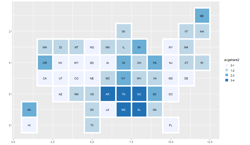<!-- --> ] --- count: false ## Cartogram heatmaps with statebins package .panel1-statebins2-non_seq[ ``` r WaPo_data2 %>% statebins( value_col = "avgshare2", ggplot2_scale_function = scale_fill_brewer, ) + * theme_statebins() ``` ] .panel2-statebins2-non_seq[ 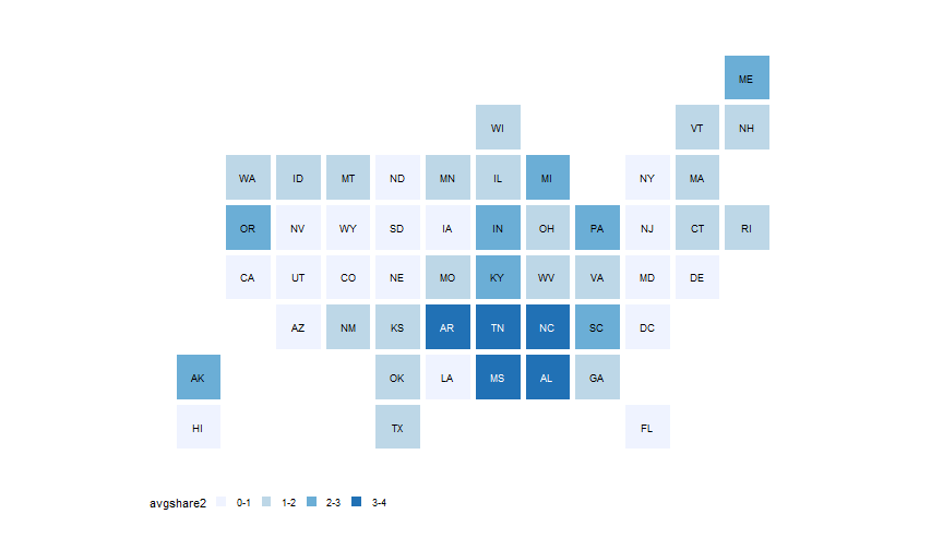<!-- --> ] --- count: false ## Cartogram heatmaps with statebins package .panel1-statebins2-non_seq[ ``` r WaPo_data2 %>% statebins( value_col = "avgshare2", ggplot2_scale_function = scale_fill_brewer, * round = TRUE ) + theme_statebins() ``` ] .panel2-statebins2-non_seq[ 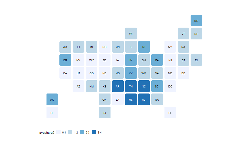<!-- --> ] --- count: false ## Cartogram heatmaps with statebins package .panel1-statebins2-non_seq[ ``` r WaPo_data2 %>% statebins( value_col = "avgshare2", ggplot2_scale_function = scale_fill_brewer, round = TRUE ) + theme_statebins() + * scale_fill_brewer( * palette = "Blues", * labels = c("Smallest\nshare", "", "", "Largest"), * name = "Share of job loss due to trade") ``` ] .panel2-statebins2-non_seq[ 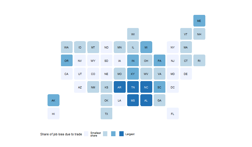<!-- --> ] --- count: false ## Cartogram heatmaps with statebins package .panel1-statebins2-non_seq[ ``` r WaPo_data2 %>% statebins( value_col = "avgshare2", ggplot2_scale_function = scale_fill_brewer, round = TRUE ) + theme_statebins() + scale_fill_brewer( palette = "Blues", labels = c("Smallest\nshare", "", "", "Largest"), name = "Share of job loss due to trade") + * guides(fill = guide_legend(title.position = "top", * label.position = "bottom")) ``` ] .panel2-statebins2-non_seq[ 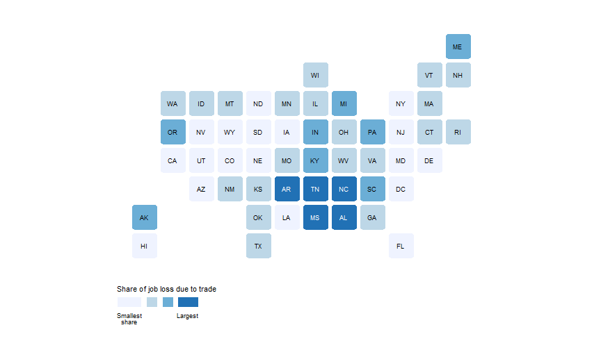<!-- --> ] --- count: false ## Cartogram heatmaps with statebins package .panel1-statebins2-non_seq[ ``` r WaPo_data2 %>% statebins( value_col = "avgshare2", ggplot2_scale_function = scale_fill_brewer, round = TRUE ) + theme_statebins() + scale_fill_brewer( palette = "Blues", labels = c("Smallest\nshare", "", "", "Largest"), name = "Share of job loss due to trade") + guides(fill = guide_legend(title.position = "top", label.position = "bottom")) + * theme(legend.position = c(0, 0.85), * legend.direction = "horizontal", * ) ``` ] .panel2-statebins2-non_seq[ 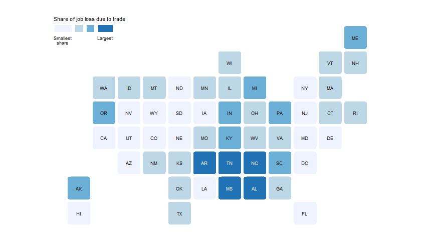<!-- --> ] --- count: false ## Cartogram heatmaps with statebins package .panel1-statebins2-non_seq[ ``` r WaPo_data2 %>% statebins( value_col = "avgshare2", ggplot2_scale_function = scale_fill_brewer, round = TRUE ) + theme_statebins() + scale_fill_brewer( palette = "Blues", labels = c("Smallest\nshare", "", "", "Largest"), name = "Share of job loss due to trade") + guides(fill = guide_legend(title.position = "top", label.position = "bottom")) + theme(legend.position = c(0, 0.85), legend.direction = "horizontal", * legend.key.height = unit(0.2, "cm"), * legend.key.width = unit(1.6, "cm") ) ``` ] .panel2-statebins2-non_seq[ 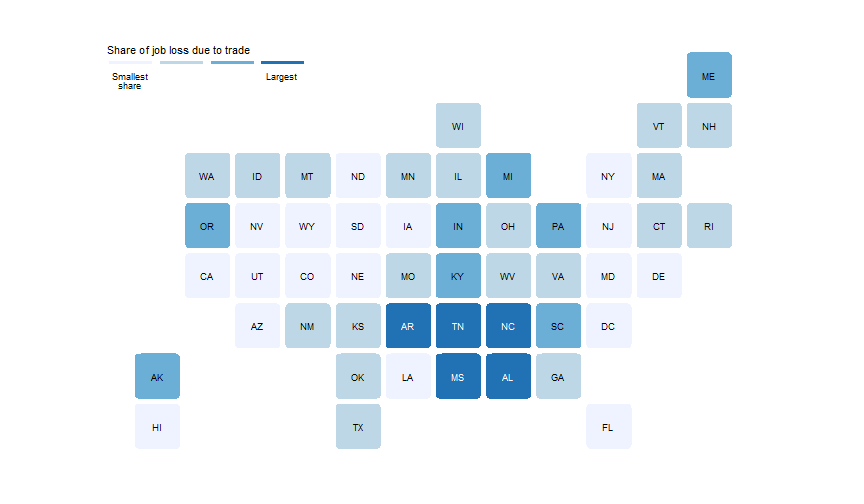<!-- --> ] <style> .panel1-statebins2-non_seq { color: black; width: 49%; hight: 32%; float: left; padding-left: 1%; font-size: 80% } .panel2-statebins2-non_seq { color: black; width: 49%; hight: 32%; float: left; padding-left: 1%; font-size: 80% } .panel3-statebins2-non_seq { color: black; width: NA%; hight: 33%; float: left; padding-left: 1%; font-size: 80% } </style> --- ## Cartogram heatmaps with statebins package - The **`statebins`** package only supports the United States data at the moment - But customizing grid should be easy to implement, like **`geofacet`** package? --- ## Tiled cartogram with tilegramsR package <img src="pictures/tileCartogram.png" width="67.5%" style="display: block; margin: auto;" /> --- count: false ## Tiled cartogram with tilegramsR package .panel1-tileCartogram1-auto[ ``` r *ec_tiles <- tilegramsR::sf_FiveThirtyEightElectoralCollege ``` ] .panel2-tileCartogram1-auto[ ] --- count: false ## Tiled cartogram with tilegramsR package .panel1-tileCartogram1-auto[ ``` r ec_tiles <- tilegramsR::sf_FiveThirtyEightElectoralCollege *class(ec_tiles) # more on sf obejct soon ``` ] .panel2-tileCartogram1-auto[ ``` [1] "sf" "data.frame" ``` ] --- count: false ## Tiled cartogram with tilegramsR package .panel1-tileCartogram1-auto[ ``` r ec_tiles <- tilegramsR::sf_FiveThirtyEightElectoralCollege class(ec_tiles) # more on sf obejct soon *ec_tiles ``` ] .panel2-tileCartogram1-auto[ ``` [1] "sf" "data.frame" ``` ``` Simple feature collection with 538 features and 3 fields Geometry type: POLYGON Dimension: XY Bounding box: xmin: 293.6239 ymin: 16.95238 xmax: 2495.803 ymax: 1661.333 CRS: NA First 10 features: FID state tilegramVa geometry 1 02 AK 3 POLYGON ((293.6239 237.3333... 2 06 CA 55 POLYGON ((352.3486 847.619,... 3 06 CA 55 POLYGON ((322.9862 796.7619... 4 06 CA 55 POLYGON ((352.3486 745.9048... 5 06 CA 55 POLYGON ((322.9862 695.0476... 6 06 CA 55 POLYGON ((352.3486 644.1905... 7 02 AK 3 POLYGON ((322.9862 288.1905... 8 02 AK 3 POLYGON ((352.3486 237.3333... 9 06 CA 55 POLYGON ((411.0734 949.3333... 10 06 CA 55 POLYGON ((381.711 898.4762,... ``` ] --- count: false ## Tiled cartogram with tilegramsR package .panel1-tileCartogram1-auto[ ``` r ec_tiles <- tilegramsR::sf_FiveThirtyEightElectoralCollege class(ec_tiles) # more on sf obejct soon ec_tiles %>% * left_join(WaPo_data2, by = c("state" = "stab")) ``` ] .panel2-tileCartogram1-auto[ ``` [1] "sf" "data.frame" ``` ``` Simple feature collection with 538 features and 6 fields Geometry type: POLYGON Dimension: XY Bounding box: xmin: 293.6239 ymin: 16.95238 xmax: 2495.803 ymax: 1661.333 CRS: NA First 10 features: FID state tilegramVa state.y avgshare avgshare2 1 02 AK 3 Alaska 1.88 2-3 2 06 CA 55 California 0.72 0-1 3 06 CA 55 California 0.72 0-1 4 06 CA 55 California 0.72 0-1 5 06 CA 55 California 0.72 0-1 6 06 CA 55 California 0.72 0-1 7 02 AK 3 Alaska 1.88 2-3 8 02 AK 3 Alaska 1.88 2-3 9 06 CA 55 California 0.72 0-1 10 06 CA 55 California 0.72 0-1 geometry 1 POLYGON ((293.6239 237.3333... 2 POLYGON ((352.3486 847.619,... 3 POLYGON ((322.9862 796.7619... 4 POLYGON ((352.3486 745.9048... 5 POLYGON ((322.9862 695.0476... 6 POLYGON ((352.3486 644.1905... 7 POLYGON ((322.9862 288.1905... 8 POLYGON ((352.3486 237.3333... 9 POLYGON ((411.0734 949.3333... 10 POLYGON ((381.711 898.4762,... ``` ] --- count: false ## Tiled cartogram with tilegramsR package .panel1-tileCartogram1-auto[ ``` r ec_tiles <- tilegramsR::sf_FiveThirtyEightElectoralCollege class(ec_tiles) # more on sf obejct soon ec_tiles %>% left_join(WaPo_data2, by = c("state" = "stab")) -> * ec_tiles ``` ] .panel2-tileCartogram1-auto[ ``` [1] "sf" "data.frame" ``` ] --- count: false ## Tiled cartogram with tilegramsR package .panel1-tileCartogram1-auto[ ``` r ec_tiles <- tilegramsR::sf_FiveThirtyEightElectoralCollege class(ec_tiles) # more on sf obejct soon ec_tiles %>% left_join(WaPo_data2, by = c("state" = "stab")) -> ec_tiles *state_tiles <- sf_FiveThirtyEightElectoralCollege.states # state polygons for drawing borders ``` ] .panel2-tileCartogram1-auto[ ``` [1] "sf" "data.frame" ``` ] --- count: false ## Tiled cartogram with tilegramsR package .panel1-tileCartogram1-auto[ ``` r ec_tiles <- tilegramsR::sf_FiveThirtyEightElectoralCollege class(ec_tiles) # more on sf obejct soon ec_tiles %>% left_join(WaPo_data2, by = c("state" = "stab")) -> ec_tiles state_tiles <- sf_FiveThirtyEightElectoralCollege.states # state polygons for drawing borders *ec_centers <- sf_FiveThirtyEightElectoralCollege.centers # state centroids for drawing labels ``` ] .panel2-tileCartogram1-auto[ ``` [1] "sf" "data.frame" ``` ] <style> .panel1-tileCartogram1-auto { color: black; width: 88.2%; hight: 32%; float: top; padding-left: 1%; font-size: 80% } .panel2-tileCartogram1-auto { color: black; width: 9.8%; hight: 32%; float: top; padding-left: 1%; font-size: 80% } .panel3-tileCartogram1-auto { color: black; width: NA%; hight: 33%; float: top; padding-left: 1%; font-size: 80% } </style> --- count: false ## Tiled cartogram with tilegramsR package .panel1-tileCartogram2-non_seq[ ``` r ggplot() + theme_void() ``` ] .panel2-tileCartogram2-non_seq[ <!-- --> ] --- count: false ## Tiled cartogram with tilegramsR package .panel1-tileCartogram2-non_seq[ ``` r ggplot() + theme_void() + * geom_sf( * data = ec_tiles, * ) ``` ] .panel2-tileCartogram2-non_seq[ 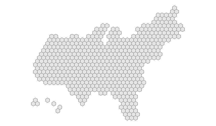<!-- --> ] --- count: false ## Tiled cartogram with tilegramsR package .panel1-tileCartogram2-non_seq[ ``` r ggplot() + theme_void() + geom_sf( data = ec_tiles, * aes( * fill = avgshare2, * ) ) ``` ] .panel2-tileCartogram2-non_seq[ 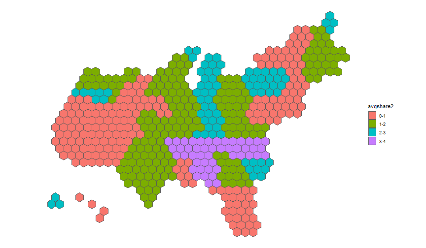<!-- --> ] --- count: false ## Tiled cartogram with tilegramsR package .panel1-tileCartogram2-non_seq[ ``` r ggplot() + theme_void() + geom_sf( data = ec_tiles, aes( fill = avgshare2, * color = avgshare2 ) ) ``` ] .panel2-tileCartogram2-non_seq[ <!-- --> ] --- count: false ## Tiled cartogram with tilegramsR package .panel1-tileCartogram2-non_seq[ ``` r ggplot() + theme_void() + geom_sf( data = ec_tiles, aes( fill = avgshare2, color = avgshare2 ) ) + * scale_fill_brewer(palette = "Blues", * name = "Share of job loss\ndue to trade") ``` ] .panel2-tileCartogram2-non_seq[ 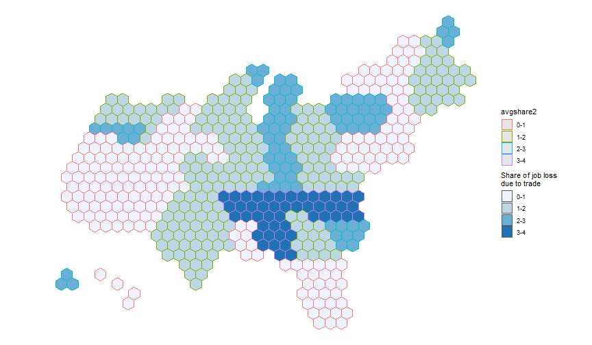<!-- --> ] --- count: false ## Tiled cartogram with tilegramsR package .panel1-tileCartogram2-non_seq[ ``` r ggplot() + theme_void() + geom_sf( data = ec_tiles, aes( fill = avgshare2, color = avgshare2 ) ) + scale_fill_brewer(palette = "Blues", name = "Share of job loss\ndue to trade") + * scale_color_brewer(palette = "Blues", * name = "Share of job loss\ndue to trade") ``` ] .panel2-tileCartogram2-non_seq[ 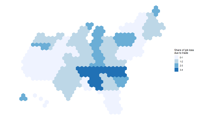<!-- --> ] --- count: false ## Tiled cartogram with tilegramsR package .panel1-tileCartogram2-non_seq[ ``` r ggplot() + theme_void() + geom_sf( data = ec_tiles, aes( fill = avgshare2, color = avgshare2 ) ) + scale_fill_brewer(palette = "Blues", name = "Share of job loss\ndue to trade") + scale_color_brewer(palette = "Blues", name = "Share of job loss\ndue to trade") + * geom_sf_text( * data = ec_centers, * aes(label = state) * ) ``` ] .panel2-tileCartogram2-non_seq[ <!-- --> ] --- count: false ## Tiled cartogram with tilegramsR package .panel1-tileCartogram2-non_seq[ ``` r ggplot() + theme_void() + geom_sf( data = ec_tiles, aes( fill = avgshare2, color = avgshare2 ) ) + scale_fill_brewer(palette = "Blues", name = "Share of job loss\ndue to trade") + scale_color_brewer(palette = "Blues", name = "Share of job loss\ndue to trade") + geom_sf_text( data = ec_centers, aes(label = state) ) + * geom_sf( * data = state_tiles, * color = "white", alpha = 0 * ) ``` ] .panel2-tileCartogram2-non_seq[ 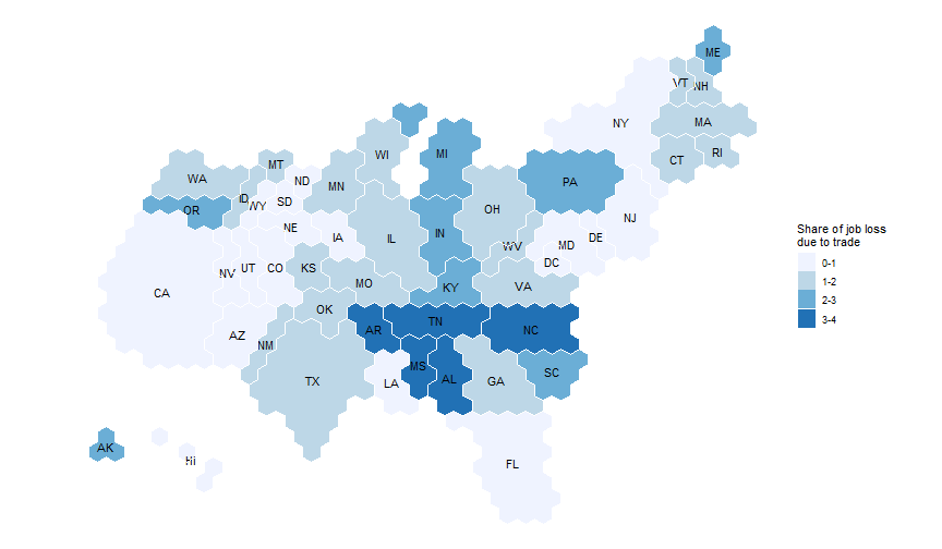<!-- --> ] --- count: false ## Tiled cartogram with tilegramsR package .panel1-tileCartogram2-non_seq[ ``` r ggplot() + theme_void() + geom_sf( data = ec_tiles, aes( fill = avgshare2, color = avgshare2 ) ) + scale_fill_brewer(palette = "Blues", name = "Share of job loss\ndue to trade") + scale_color_brewer(palette = "Blues", name = "Share of job loss\ndue to trade") + geom_sf_text( data = ec_centers, aes(label = state) ) + geom_sf( data = state_tiles, color = "white", alpha = 0 ) + * theme(legend.position = c(0.925, 0.25)) ``` ] .panel2-tileCartogram2-non_seq[ 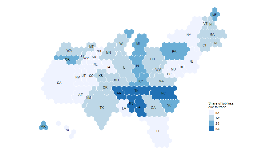<!-- --> ] <style> .panel1-tileCartogram2-non_seq { color: black; width: 49%; hight: 32%; float: left; padding-left: 1%; font-size: 80% } .panel2-tileCartogram2-non_seq { color: black; width: 49%; hight: 32%; float: left; padding-left: 1%; font-size: 80% } .panel3-tileCartogram2-non_seq { color: black; width: NA%; hight: 33%; float: left; padding-left: 1%; font-size: 80% } </style> --- ## Final thoughts about tiled cartograms - Why hexagos? [Because hexagons are the bestagons](https://www.youtube.com/watch?v=thOifuHs6eY) -- - To my knowledge, there is no existing algorithm to automatically generate the tile cartogram layouts -- - I'm trying to develop a function/package to do that: inspirations from using neural networks/ genetic algorithms to solve the [Tetris game](https://cs229.stanford.edu/proj2015/238_report.pdf) --- ## Introduction to spatial data in R - Numerous spatial data formats -- - **`.shp`** (shapefile; the most common); `.geojson`, `.json`; `.gml`; `.csv`; `.tiff`... -- - Countless packages to work with spatial data -- - Recent package **`sf`** allows geospatial data to be stored in data frames -- - Well integrated with `tidyverse` -- - Many packages to draw maps -- - **`tmap`** allows easy visualization of static and interactive maps -- - Also employs the "grammar of graphics" --- ## Introduction to spatial data in R - Grammar of graphics in **`tmap`**: | ggplot2 | tmap -- | --------------- | --------------- Data |`ggplot(...) +` |`tm_shape(...) +` Layers |`geom_...(...) +` |`tm_...(...) +` Small Multiples |`facet_grid(...)` |`tm_facets(...)` Layout |`theme(...)` |`tm_layout(...)` --- ## Introduction to spatial data in R - Before plotting choropleth maps, we need to find the appropriate shapefile -- - Download the US shapefile [here](https://www.census.gov/geographies/mapping-files/time-series/geo/carto-boundary-file.html) --- count: false ## Choropleth maps with sf and tmap .panel1-tmap1-auto[ ``` r *us_shp <- st_read("data/cb_2018_us_state_20m/cb_2018_us_state_20m.shp") ``` ] .panel2-tmap1-auto[ ``` Reading layer `cb_2018_us_state_20m' from data source `D:\Google Drive\Phd UW\Courses\5th year\CS&SS 569 - Visualizing Data and Models\Labs\Lab6\data\cb_2018_us_state_20m\cb_2018_us_state_20m.shp' using driver `ESRI Shapefile' Simple feature collection with 52 features and 9 fields Geometry type: MULTIPOLYGON Dimension: XY Bounding box: xmin: -179.1743 ymin: 17.91377 xmax: 179.7739 ymax: 71.35256 Geodetic CRS: NAD83 ``` ] --- count: false ## Choropleth maps with sf and tmap .panel1-tmap1-auto[ ``` r us_shp <- st_read("data/cb_2018_us_state_20m/cb_2018_us_state_20m.shp") *class(us_shp) ``` ] .panel2-tmap1-auto[ ``` Reading layer `cb_2018_us_state_20m' from data source `D:\Google Drive\Phd UW\Courses\5th year\CS&SS 569 - Visualizing Data and Models\Labs\Lab6\data\cb_2018_us_state_20m\cb_2018_us_state_20m.shp' using driver `ESRI Shapefile' Simple feature collection with 52 features and 9 fields Geometry type: MULTIPOLYGON Dimension: XY Bounding box: xmin: -179.1743 ymin: 17.91377 xmax: 179.7739 ymax: 71.35256 Geodetic CRS: NAD83 ``` ``` [1] "sf" "data.frame" ``` ] --- count: false ## Choropleth maps with sf and tmap .panel1-tmap1-auto[ ``` r us_shp <- st_read("data/cb_2018_us_state_20m/cb_2018_us_state_20m.shp") class(us_shp) *head(as_tibble(us_shp)) ``` ] .panel2-tmap1-auto[ ``` Reading layer `cb_2018_us_state_20m' from data source `D:\Google Drive\Phd UW\Courses\5th year\CS&SS 569 - Visualizing Data and Models\Labs\Lab6\data\cb_2018_us_state_20m\cb_2018_us_state_20m.shp' using driver `ESRI Shapefile' Simple feature collection with 52 features and 9 fields Geometry type: MULTIPOLYGON Dimension: XY Bounding box: xmin: -179.1743 ymin: 17.91377 xmax: 179.7739 ymax: 71.35256 Geodetic CRS: NAD83 ``` ``` [1] "sf" "data.frame" ``` ``` # A tibble: 6 × 10 STATEFP STATENS AFFGEOID GEOID STUSPS NAME LSAD ALAND AWATER <chr> <chr> <chr> <chr> <chr> <chr> <chr> <dbl> <dbl> 1 24 01714934 0400000US24 24 MD Maryland 00 2.52e10 6.98e 9 2 19 01779785 0400000US19 19 IA Iowa 00 1.45e11 1.08e 9 3 10 01779781 0400000US10 10 DE Delaware 00 5.05e 9 1.40e 9 4 39 01085497 0400000US39 39 OH Ohio 00 1.06e11 1.03e10 5 42 01779798 0400000US42 42 PA Pennsylvania 00 1.16e11 3.39e 9 6 31 01779792 0400000US31 31 NE Nebraska 00 1.99e11 1.37e 9 # ℹ 1 more variable: geometry <MULTIPOLYGON [°]> ``` ] <style> .panel1-tmap1-auto { color: black; width: 39.2%; hight: 32%; float: left; padding-left: 1%; font-size: 80% } .panel2-tmap1-auto { color: black; width: 58.8%; hight: 32%; float: left; padding-left: 1%; font-size: 80% } .panel3-tmap1-auto { color: black; width: NA%; hight: 33%; float: left; padding-left: 1%; font-size: 80% } </style> --- count: false ## Choropleth maps with sf and tmap .panel1-tmap2-auto[ ``` r *us_shp ``` ] .panel2-tmap2-auto[ ``` Simple feature collection with 52 features and 9 fields Geometry type: MULTIPOLYGON Dimension: XY Bounding box: xmin: -179.1743 ymin: 17.91377 xmax: 179.7739 ymax: 71.35256 Geodetic CRS: NAD83 First 10 features: STATEFP STATENS AFFGEOID GEOID STUSPS NAME LSAD ALAND 1 24 01714934 0400000US24 24 MD Maryland 00 25151100280 2 19 01779785 0400000US19 19 IA Iowa 00 144661267977 3 10 01779781 0400000US10 10 DE Delaware 00 5045925646 4 39 01085497 0400000US39 39 OH Ohio 00 105828882568 5 42 01779798 0400000US42 42 PA Pennsylvania 00 115884442321 6 31 01779792 0400000US31 31 NE Nebraska 00 198956658395 7 53 01779804 0400000US53 53 WA Washington 00 172112588220 8 72 01779808 0400000US72 72 PR Puerto Rico 00 8868896030 9 01 01779775 0400000US01 01 AL Alabama 00 131174048583 10 05 00068085 0400000US05 05 AR Arkansas 00 134768872727 AWATER geometry 1 6979966958 MULTIPOLYGON (((-76.04621 3... 2 1084180812 MULTIPOLYGON (((-96.62187 4... 3 1399985648 MULTIPOLYGON (((-75.77379 3... 4 10268850702 MULTIPOLYGON (((-82.86334 4... 5 3394589990 MULTIPOLYGON (((-80.51989 4... 6 1371829134 MULTIPOLYGON (((-104.0531 4... 7 12559278850 MULTIPOLYGON (((-123.2371 4... 8 4922382562 MULTIPOLYGON (((-65.34207 1... 9 4593327154 MULTIPOLYGON (((-88.46866 3... 10 2962859592 MULTIPOLYGON (((-94.61792 3... ``` ] --- count: false ## Choropleth maps with sf and tmap .panel1-tmap2-auto[ ``` r us_shp %>% * left_join(WaPo_data, by=c("NAME" = "state")) ``` ] .panel2-tmap2-auto[ ``` Simple feature collection with 52 features and 31 fields Geometry type: MULTIPOLYGON Dimension: XY Bounding box: xmin: -179.1743 ymin: 17.91377 xmax: 179.7739 ymax: 71.35256 Geodetic CRS: NAD83 First 10 features: STATEFP STATENS AFFGEOID GEOID STUSPS NAME LSAD ALAND 1 24 01714934 0400000US24 24 MD Maryland 00 25151100280 2 19 01779785 0400000US19 19 IA Iowa 00 144661267977 3 10 01779781 0400000US10 10 DE Delaware 00 5045925646 4 39 01085497 0400000US39 39 OH Ohio 00 105828882568 5 42 01779798 0400000US42 42 PA Pennsylvania 00 115884442321 6 31 01779792 0400000US31 31 NE Nebraska 00 198956658395 7 53 01779804 0400000US53 53 WA Washington 00 172112588220 8 72 01779808 0400000US72 72 PR Puerto Rico 00 8868896030 9 01 01779775 0400000US01 01 AL Alabama 00 131174048583 10 05 00068085 0400000US05 05 AR Arkansas 00 134768872727 AWATER stab share_cut1994 share_cut1995 share_cut1996 share_cut1997 1 6979966958 MD 0.4 1.1 0.7 0.4 2 1084180812 IA 0.1 0.4 0.5 0.6 3 1399985648 DE 0.6 0.0 0.0 0.0 4 10268850702 OH 0.6 0.8 0.6 1.0 5 3394589990 PA 1.5 1.4 2.0 1.7 6 1371829134 NE 0.0 0.2 0.7 0.1 7 12559278850 WA 1.0 1.2 0.5 0.4 8 4922382562 <NA> NA NA NA NA 9 4593327154 AL 1.1 2.4 5.2 4.6 10 2962859592 AR 1.6 1.3 1.6 2.7 share_cut1998 share_cut1999 share_cut2000 share_cut2001 share_cut2002 1 0.5 0.4 0.3 0.1 0.3 2 0.1 0.5 0.1 0.6 0.9 3 0.0 0.4 0.0 0.0 0.0 4 0.5 1.0 0.9 1.3 2.5 5 1.5 1.3 1.4 3.6 2.8 6 0.1 0.2 1.0 0.0 0.6 7 1.0 0.7 2.5 1.4 9.4 8 NA NA NA NA NA 9 3.5 5.6 2.5 2.8 6.5 10 2.7 2.8 0.6 3.1 3.9 share_cut2003 share_cut2004 share_cut2005 share_cut2006 share_cut2007 1 1.1 0.1 0.5 0.7 0.8 2 0.9 1.0 0.6 2.4 0.9 3 1.0 0.9 0.7 0.4 0.1 4 1.9 1.4 0.9 2.9 2.0 5 2.8 1.2 1.5 0.9 1.6 6 2.0 1.2 0.2 0.2 0.9 7 1.3 3.4 0.6 0.4 0.6 8 NA NA NA NA NA 9 2.2 2.1 1.2 3.3 2.6 10 3.6 1.1 2.3 3.8 4.9 share_cut2008 share_cut2009 share_cut2010 share_cut2011 share_cut2012 1 0.5 0.2 0.6 0.8 0.3 2 0.8 2.3 1.4 1.4 0.2 3 0.0 5.4 0.0 0.0 0.0 4 2.2 5.0 2.8 1.0 1.3 5 1.0 2.6 2.5 0.9 1.1 6 0.3 1.3 0.3 1.1 0.1 7 0.7 2.2 1.6 1.1 1.0 8 NA NA NA NA NA 9 3.9 4.3 3.6 0.4 0.7 10 3.2 3.0 3.3 2.4 3.9 share_cut2013 avgshare geometry 1 0.1 0.47 MULTIPOLYGON (((-76.04621 3... 2 1.1 0.89 MULTIPOLYGON (((-96.62187 4... 3 0.1 0.53 MULTIPOLYGON (((-75.77379 3... 4 0.4 1.72 MULTIPOLYGON (((-82.86334 4... 5 0.8 1.79 MULTIPOLYGON (((-80.51989 4... 6 0.5 0.62 MULTIPOLYGON (((-104.0531 4... 7 0.7 1.69 MULTIPOLYGON (((-123.2371 4... 8 NA NA MULTIPOLYGON (((-65.34207 1... 9 0.6 3.22 MULTIPOLYGON (((-88.46866 3... 10 0.5 2.89 MULTIPOLYGON (((-94.61792 3... ``` ] --- count: false ## Choropleth maps with sf and tmap .panel1-tmap2-auto[ ``` r us_shp %>% left_join(WaPo_data, by=c("NAME" = "state")) %>% * tigris::shift_geometry() # rescale AK, HI, PR ``` ] .panel2-tmap2-auto[ ``` Simple feature collection with 52 features and 31 fields Geometry type: MULTIPOLYGON Dimension: XY Bounding box: xmin: -3112200 ymin: -1697728 xmax: 2258154 ymax: 1558935 Projected CRS: USA_Contiguous_Albers_Equal_Area_Conic First 10 features: STATEFP STATENS AFFGEOID GEOID STUSPS NAME LSAD ALAND 1 24 01714934 0400000US24 24 MD Maryland 00 25151100280 2 19 01779785 0400000US19 19 IA Iowa 00 144661267977 3 10 01779781 0400000US10 10 DE Delaware 00 5045925646 4 39 01085497 0400000US39 39 OH Ohio 00 105828882568 5 42 01779798 0400000US42 42 PA Pennsylvania 00 115884442321 6 31 01779792 0400000US31 31 NE Nebraska 00 198956658395 7 53 01779804 0400000US53 53 WA Washington 00 172112588220 8 01 01779775 0400000US01 01 AL Alabama 00 131174048583 9 05 00068085 0400000US05 05 AR Arkansas 00 134768872727 10 35 00897535 0400000US35 35 NM New Mexico 00 314196306401 AWATER stab share_cut1994 share_cut1995 share_cut1996 share_cut1997 1 6979966958 MD 0.4 1.1 0.7 0.4 2 1084180812 IA 0.1 0.4 0.5 0.6 3 1399985648 DE 0.6 0.0 0.0 0.0 4 10268850702 OH 0.6 0.8 0.6 1.0 5 3394589990 PA 1.5 1.4 2.0 1.7 6 1371829134 NE 0.0 0.2 0.7 0.1 7 12559278850 WA 1.0 1.2 0.5 0.4 8 4593327154 AL 1.1 2.4 5.2 4.6 9 2962859592 AR 1.6 1.3 1.6 2.7 10 728776523 NM 1.4 0.8 0.9 3.0 share_cut1998 share_cut1999 share_cut2000 share_cut2001 share_cut2002 1 0.5 0.4 0.3 0.1 0.3 2 0.1 0.5 0.1 0.6 0.9 3 0.0 0.4 0.0 0.0 0.0 4 0.5 1.0 0.9 1.3 2.5 5 1.5 1.3 1.4 3.6 2.8 6 0.1 0.2 1.0 0.0 0.6 7 1.0 0.7 2.5 1.4 9.4 8 3.5 5.6 2.5 2.8 6.5 9 2.7 2.8 0.6 3.1 3.9 10 1.4 4.5 0.4 0.3 1.7 share_cut2003 share_cut2004 share_cut2005 share_cut2006 share_cut2007 1 1.1 0.1 0.5 0.7 0.8 2 0.9 1.0 0.6 2.4 0.9 3 1.0 0.9 0.7 0.4 0.1 4 1.9 1.4 0.9 2.9 2.0 5 2.8 1.2 1.5 0.9 1.6 6 2.0 1.2 0.2 0.2 0.9 7 1.3 3.4 0.6 0.4 0.6 8 2.2 2.1 1.2 3.3 2.6 9 3.6 1.1 2.3 3.8 4.9 10 0.5 0.1 0.1 0.1 0.0 share_cut2008 share_cut2009 share_cut2010 share_cut2011 share_cut2012 1 0.5 0.2 0.6 0.8 0.3 2 0.8 2.3 1.4 1.4 0.2 3 0.0 5.4 0.0 0.0 0.0 4 2.2 5.0 2.8 1.0 1.3 5 1.0 2.6 2.5 0.9 1.1 6 0.3 1.3 0.3 1.1 0.1 7 0.7 2.2 1.6 1.1 1.0 8 3.9 4.3 3.6 0.4 0.7 9 3.2 3.0 3.3 2.4 3.9 10 4.1 1.7 1.9 0.1 0.8 share_cut2013 avgshare geometry 1 0.1 0.47 MULTIPOLYGON (((1722285 240... 2 1.1 0.89 MULTIPOLYGON (((-50588.83 5... 3 0.1 0.53 MULTIPOLYGON (((1705278 431... 4 0.4 1.72 MULTIPOLYGON (((1081987 544... 5 0.8 1.79 MULTIPOLYGON (((1287712 486... 6 0.5 0.62 MULTIPOLYGON (((-670097.4 4... 7 0.7 1.69 MULTIPOLYGON (((-2000238 15... 8 0.6 3.22 MULTIPOLYGON (((708460.5 -5... 9 0.5 2.89 MULTIPOLYGON (((122656.3 -1... 10 0.0 1.26 MULTIPOLYGON (((-1226428 -5... ``` ] --- count: false ## Choropleth maps with sf and tmap .panel1-tmap2-auto[ ``` r us_shp %>% left_join(WaPo_data, by=c("NAME" = "state")) %>% tigris::shift_geometry() -> # rescale AK, HI, PR * us_shp2 ``` ] .panel2-tmap2-auto[ ] <style> .panel1-tmap2-auto { color: black; width: 39.2%; hight: 32%; float: left; padding-left: 1%; font-size: 80% } .panel2-tmap2-auto { color: black; width: 58.8%; hight: 32%; float: left; padding-left: 1%; font-size: 80% } .panel3-tmap2-auto { color: black; width: NA%; hight: 33%; float: left; padding-left: 1%; font-size: 80% } </style> --- count: false ## Choropleth maps with sf and tmap .panel1-tmap3-non_seq[ ``` r tm_shape(us_shp2) + tm_polygons( ) ``` ] .panel2-tmap3-non_seq[ 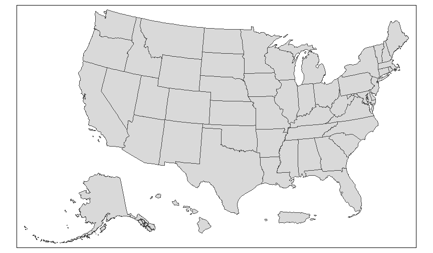<!-- --> ] --- count: false ## Choropleth maps with sf and tmap .panel1-tmap3-non_seq[ ``` r tm_shape(us_shp2) + tm_polygons( * col = "avgshare", * palette = "Blues", ) ``` ] .panel2-tmap3-non_seq[ 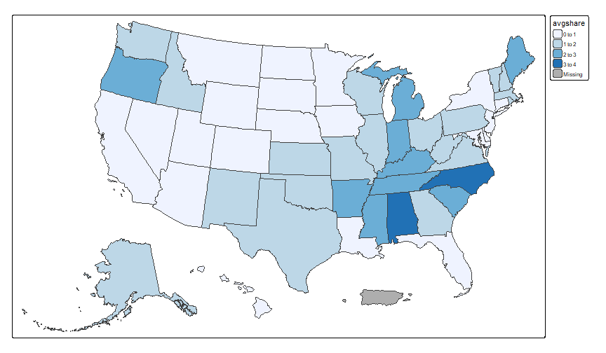<!-- --> ] --- count: false ## Choropleth maps with sf and tmap .panel1-tmap3-non_seq[ ``` r tm_shape(us_shp2) + tm_polygons( col = "avgshare", palette = "Blues", * border.col = "white", ) ``` ] .panel2-tmap3-non_seq[ 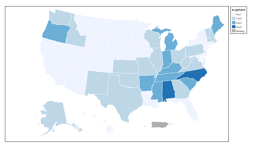<!-- --> ] --- count: false ## Choropleth maps with sf and tmap .panel1-tmap3-non_seq[ ``` r tm_shape(us_shp2) + tm_polygons( col = "avgshare", palette = "Blues", border.col = "white", ) + * tm_text( * text = "STUSPS", * ) ``` ] .panel2-tmap3-non_seq[ 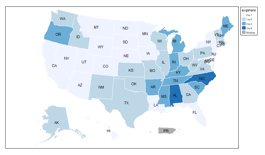<!-- --> ] --- count: false ## Choropleth maps with sf and tmap .panel1-tmap3-non_seq[ ``` r tm_shape(us_shp2) + tm_polygons( col = "avgshare", palette = "Blues", border.col = "white", ) + tm_text( text = "STUSPS", * size = "avgshare", * legend.size.show = FALSE ) ``` ] .panel2-tmap3-non_seq[ <!-- --> ] --- count: false ## Choropleth maps with sf and tmap .panel1-tmap3-non_seq[ ``` r tm_shape(us_shp2) + tm_polygons( col = "avgshare", palette = "Blues", border.col = "white", ) + tm_text( text = "STUSPS", size = "avgshare", legend.size.show = FALSE ) + * tm_layout( * frame = FALSE, * ) ``` ] .panel2-tmap3-non_seq[ 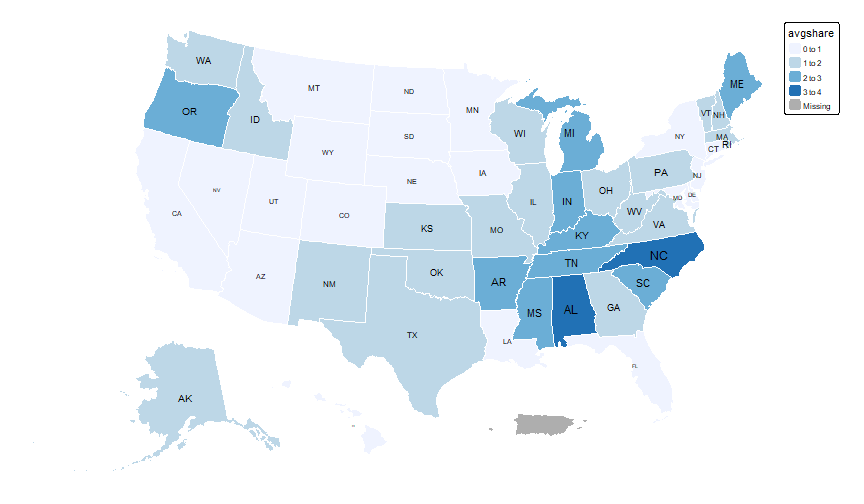<!-- --> ] --- count: false ## Choropleth maps with sf and tmap .panel1-tmap3-non_seq[ ``` r tm_shape(us_shp2) + tm_polygons( col = "avgshare", palette = "Blues", border.col = "white", * legend.is.portrait = FALSE, ) + tm_text( text = "STUSPS", size = "avgshare", legend.size.show = FALSE ) + tm_layout( frame = FALSE, * legend.stack = "horizontal", ) ``` ] .panel2-tmap3-non_seq[ 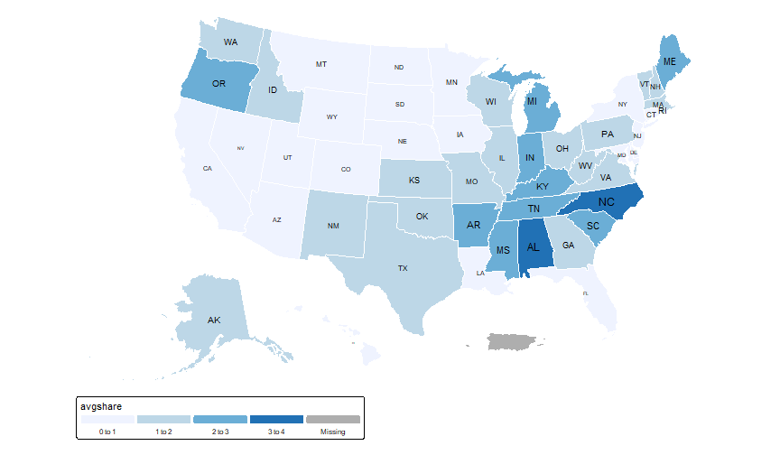<!-- --> ] --- count: false ## Choropleth maps with sf and tmap .panel1-tmap3-non_seq[ ``` r tm_shape(us_shp2) + tm_polygons( col = "avgshare", palette = "Blues", border.col = "white", legend.is.portrait = FALSE, ) + tm_text( text = "STUSPS", size = "avgshare", legend.size.show = FALSE ) + tm_layout( frame = FALSE, legend.stack = "horizontal", * legend.position = c('right', 'top'), ) ``` ] .panel2-tmap3-non_seq[ 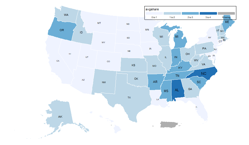<!-- --> ] --- count: false ## Choropleth maps with sf and tmap .panel1-tmap3-non_seq[ ``` r tm_shape(us_shp2) + tm_polygons( col = "avgshare", palette = "Blues", border.col = "white", legend.is.portrait = FALSE, * title = "Share of job loss due to trade", * labels = c("Smallest", "", "", "Largest share") ) + tm_text( text = "STUSPS", size = "avgshare", legend.size.show = FALSE ) + tm_layout( frame = FALSE, legend.stack = "horizontal", legend.position = c('right', 'top'), * legend.title.size = 1, * legend.text.size = 0.5 ) ``` ] .panel2-tmap3-non_seq[ 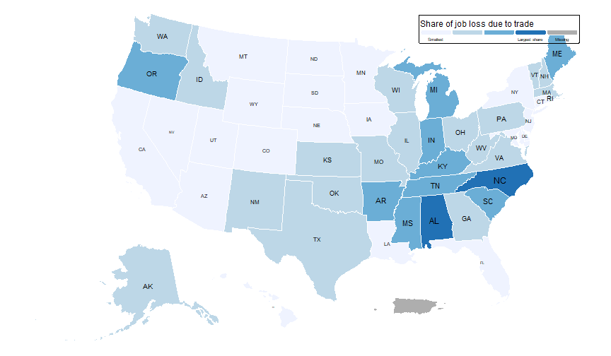<!-- --> ] <style> .panel1-tmap3-non_seq { color: black; width: 49%; hight: 32%; float: left; padding-left: 1%; font-size: 80% } .panel2-tmap3-non_seq { color: black; width: 49%; hight: 32%; float: left; padding-left: 1%; font-size: 80% } .panel3-tmap3-non_seq { color: black; width: NA%; hight: 33%; float: left; padding-left: 1%; font-size: 80% } </style> --- ## Choropleth maps with sf and tmap - To save the map: ``` r tmap_save(tmap_object, filename = "[...].pdf") ``` --- ## Choropleth maps with sf and tmap: NYC examples - Download the [Rental Housing and Demographics in NYC data](https://geodacenter.github.io/data-and-lab/nyc/) -- - Unzip it and put it in your working directory -- ``` r # load .shp file with sf nyc_shp <- st_read("data/nyc/nyc.shp") ``` ``` Reading layer `nyc' from data source `D:\Google Drive\Phd UW\Courses\5th year\CS&SS 569 - Visualizing Data and Models\Labs\Lab6\data\nyc\nyc.shp' using driver `ESRI Shapefile' Simple feature collection with 55 features and 34 fields Geometry type: MULTIPOLYGON Dimension: XY Bounding box: xmin: 913037.2 ymin: 120117 xmax: 1067549 ymax: 272751.4 Projected CRS: NAD83 / New York Long Island (ftUS) ``` --- count: false ## Choropleth maps with sf and tmap: NYC examples .panel1-nyc1-non_seq[ ``` r tm_shape(nyc_shp) + tm_polygons( ) ``` ] .panel2-nyc1-non_seq[ 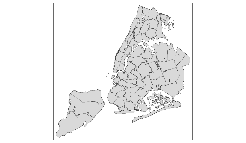<!-- --> ] --- count: false ## Choropleth maps with sf and tmap: NYC examples .panel1-nyc1-non_seq[ ``` r tm_shape(nyc_shp) + tm_polygons( * col = "rent2008", ) ``` ] .panel2-nyc1-non_seq[ 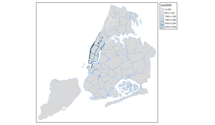<!-- --> ] --- count: false ## Choropleth maps with sf and tmap: NYC examples .panel1-nyc1-non_seq[ ``` r tm_shape(nyc_shp) + tm_polygons( col = "rent2008", * palette = "BrBG", ) ``` ] .panel2-nyc1-non_seq[ 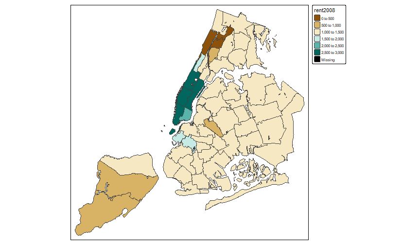<!-- --> ] --- count: false ## Choropleth maps with sf and tmap: NYC examples .panel1-nyc1-non_seq[ ``` r tm_shape(nyc_shp) + tm_polygons( col = "rent2008", palette = "BrBG", * border.col = "white", ) ``` ] .panel2-nyc1-non_seq[ 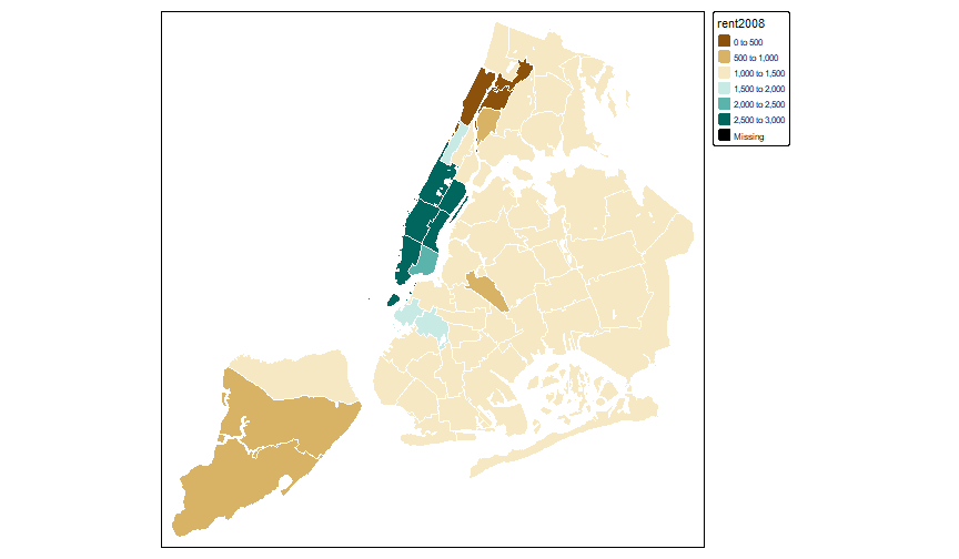<!-- --> ] --- count: false ## Choropleth maps with sf and tmap: NYC examples .panel1-nyc1-non_seq[ ``` r tm_shape(nyc_shp) + tm_polygons( col = "rent2008", palette = "BrBG", border.col = "white", * title = "Rent in 2008" ) ``` ] .panel2-nyc1-non_seq[ 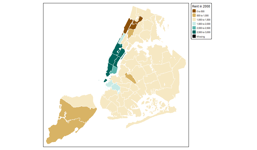<!-- --> ] --- count: false ## Choropleth maps with sf and tmap: NYC examples .panel1-nyc1-non_seq[ ``` r tm_shape(nyc_shp) + tm_polygons( col = "rent2008", palette = "BrBG", border.col = "white", title = "Rent in 2008" ) + * tm_layout(frame = FALSE) ``` ] .panel2-nyc1-non_seq[ <!-- --> ] <style> .panel1-nyc1-non_seq { color: black; width: 39.2%; hight: 32%; float: left; padding-left: 1%; font-size: 80% } .panel2-nyc1-non_seq { color: black; width: 58.8%; hight: 32%; float: left; padding-left: 1%; font-size: 80% } .panel3-nyc1-non_seq { color: black; width: NA%; hight: 33%; float: left; padding-left: 1%; font-size: 80% } </style> --- count: false ## Choropleth maps with sf and tmap: NYC examples .panel1-nyc2-auto[ ``` r ## interactive mode in tmap *tmap_mode("view") ``` ] .panel2-nyc2-auto[ ] --- count: false ## Choropleth maps with sf and tmap: NYC examples .panel1-nyc2-auto[ ``` r ## interactive mode in tmap tmap_mode("view") ## switch off spherical geometry to avoid error ## usually you don't need to do this *sf::sf_use_s2(use_s2 = FALSE) ``` ] .panel2-nyc2-auto[ ] --- count: false ## Choropleth maps with sf and tmap: NYC examples .panel1-nyc2-auto[ ``` r ## interactive mode in tmap tmap_mode("view") ## switch off spherical geometry to avoid error ## usually you don't need to do this sf::sf_use_s2(use_s2 = FALSE) ## tmap *tm_shape(nyc_shp) + tm_polygons( * col = "rent2008", * palette = "BrBG", * title = "Rent in 2008", * alpha = 0.5 * ) ``` ] .panel2-nyc2-auto[ <style>#legend01 { background: #FFFFFF; opacity: 1}</style> <div class="leaflet html-widget html-fill-item" id="htmlwidget-70f61fcc836e85972bcf" style="width:864px;height:504px;"></div> <script type="application/json" data-for="htmlwidget-70f61fcc836e85972bcf">{"x":{"options":{"crs":{"crsClass":"L.CRS.EPSG3857","code":null,"proj4def":null,"projectedBounds":null,"options":{}},"attributionControl":true},"calls":[{"method":"createMapPane","args":["tmap401",401]},{"method":"addLayersControl","args":[["Esri.WorldGrayCanvas","OpenStreetMap","Esri.WorldTopoMap"],"nyc_shp",{"collapsed":true,"autoZIndex":true,"position":"topleft"}]},{"method":"addProviderTiles","args":["Esri.WorldGrayCanvas",null,"Esri.WorldGrayCanvas",{"minZoom":0,"maxZoom":18,"maxNativeZoom":17,"tileSize":256,"subdomains":"abc","errorTileUrl":"","tms":false,"noWrap":false,"zoomOffset":0,"zoomReverse":false,"opacity":1,"zIndex":1,"detectRetina":false,"pane":"tilePane"}]},{"method":"addProviderTiles","args":["OpenStreetMap",null,"OpenStreetMap",{"minZoom":0,"maxZoom":18,"maxNativeZoom":17,"tileSize":256,"subdomains":"abc","errorTileUrl":"","tms":false,"noWrap":false,"zoomOffset":0,"zoomReverse":false,"opacity":1,"zIndex":1,"detectRetina":false,"pane":"tilePane"}]},{"method":"addProviderTiles","args":["Esri.WorldTopoMap",null,"Esri.WorldTopoMap",{"minZoom":0,"maxZoom":18,"maxNativeZoom":17,"tileSize":256,"subdomains":"abc","errorTileUrl":"","tms":false,"noWrap":false,"zoomOffset":0,"zoomReverse":false,"opacity":1,"zIndex":1,"detectRetina":false,"pane":"tilePane"}]},{"method":"addPolygons","args":[[[[{"lng":[-74.07838400002191,-74.07688399996789,-74.07588400000149,-74.07528399997989,-74.07608400000871,-74.07568399999431,-74.07508399997269,-74.0751839999763,-74.0743840000171,-74.07338399998108,-74.07278400002912,-74.0728840000327,-74.07218400000748,-74.07138399997866,-74.07068400002309,-74.07042299998723,-74.07014800001215,-74.06970000000715,-74.06897500001584,-74.06906699997459,-74.06883400002609,-74.06892700002525,-74.06851599998399,-74.06855199997693,-74.06860100000796,-74.06759799998991,-74.06588199997825,-74.06461399997157,-74.06585599997173,-74.06495899999095,-74.06388899998026,-74.06280500003034,-74.06404500001932,-74.06365700000254,-74.06360600002995,-74.06276000002175,-74.06167100000899,-74.06034500002529,-74.06034199997367,-74.06034300001407,-74.06020299999511,-74.05969500000188,-74.05908400002305,-74.05901300000795,-74.05715800001774,-74.05713299998202,-74.05678400000983,-74.05662699999999,-74.05717399996817,-74.05757599999379,-74.06033499996924,-74.0604279999684,-74.06495199998653,-74.06514499998929,-74.06548899996827,-74.06585700001216,-74.06620300000233,-74.06655000003293,-74.06696100000457,-74.06860199997874,-74.06877599997942,-74.07397699999827,-74.07436599998583,-74.07465600001018,-74.07538000003069,-74.07635199997937,-74.07654699999335,-74.07730299998437,-74.07754000002494,-74.07792900001249,-74.07937800002429,-74.08130900002283,-74.08132400000248,-74.08257599998909,-74.08346099997222,-74.08443299999053,-74.08477800000992,-74.08486899999787,-74.08516699999748,-74.08566299999305,-74.08602999999651,-74.08678500001675,-74.08736799997787,-74.08753100002134,-74.08844700000419,-74.08928800001918,-74.09023799998376,-74.0909719999907,-74.0943390000326,-74.09794699999823,-74.09829299998843,-74.09984900000825,-74.10032399999055,-74.10142700001218,-74.1023560000331,-74.10354400000907,-74.10453800001144,-74.10561800000855,-74.10544800003028,-74.10603799999585,-74.10651700000055,-74.10710599999533,-74.10754699999588,-74.10841699999938,-74.10922000001018,-74.10984799997988,-74.10987800000882,-74.11015900001755,-74.11021400001256,-74.1102970000253,-74.11073300003264,-74.11110899998214,-74.11153599997384,-74.11186100002035,-74.11291299999976,-74.11298799996766,-74.11365499998192,-74.1138929999933,-74.11687599997121,-74.11763300000266,-74.11845500001556,-74.11880100000573,-74.11960100003455,-74.12111599999861,-74.12146199998878,-74.12252299998383,-74.1227369999999,-74.12394800000034,-74.12641299999861,-74.12738599998771,-74.1280339999999,-74.12889900001016,-74.12995799999402,-74.13108200002893,-74.13224899999157,-74.13311400000184,-74.13397799997169,-74.13501600001186,-74.1359019999658,-74.13693899996555,-74.13804199998718,-74.13903599998956,-74.13990000002904,-74.14087300001813,-74.14180199996942,-74.14277500002814,-74.14398499998816,-74.14554100000801,-74.14722600001996,-74.1492330000268,-74.14968600002503,-74.15024799997283,-74.1506359999896,-74.15259900002829,-74.15322400001597,-74.1538060000063,-74.15471200000272,-74.15503600000882,-74.15624400002727,-74.15756000002453,-74.15714699997206,-74.15706000000652,-74.15684300000846,-74.15885200002653,-74.15960800001753,-74.16029799998668,-74.16131200003157,-74.16329800002511,-74.1642479999897,-74.16528400001866,-74.16729199999629,-74.16802600000324,-74.16845700001737,-74.16860900003398,-74.16975299997213,-74.17709400001236,-74.17776400000864,-74.17851900002886,-74.18104499998616,-74.18313500000573,-74.18331199998843,-74.18596799997826,-74.18618400000554,-74.19192799997012,-74.19242399996571,-74.19574899998102,-74.19588899999999,-74.19545000001064,-74.19485200000024,-74.19478799998959,-74.19329299999841,-74.19059600002241,-74.19049699998961,-74.18940000000161,-74.18739299999477,-74.18709599996598,-74.1880009999916,-74.18650100000721,-74.18549799998918,-74.184198000012,-74.18409599999717,-74.18109299997674,-74.18099200000235,-74.18019100000275,-74.17909100003276,-74.17929499999275,-74.17839300001874,-74.17708999998992,-74.17608899998312,-74.17568700002711,-74.1740850000279,-74.17278499998108,-74.17238600000709,-74.17138500000029,-74.17148799998589,-74.17133299998727,-74.17078699998989,-74.17018699996827,-74.16928700000548,-74.16818699996585,-74.16778700002109,-74.16598700002588,-74.16588700002229,-74.16508699999346,-74.16488699998625,-74.16398700002347,-74.16308699999105,-74.16278100001624,-74.16128999997785,-74.16169999997869,-74.16079800000469,-74.16008799999304,-74.15888399999703,-74.15808399996821,-74.15698399999822,-74.15637500003059,-74.1547760000134,-74.15455099997047,-74.15255700000169,-74.15297299996656,-74.15127499998616,-74.15015499997368,-74.14965300001408,-74.14955399998126,-74.14973900000881,-74.14905200002168,-74.14561299999389,-74.14473500001517,-74.1438419999872,-74.14335000001404,-74.14274200001721,-74.142740000006,-74.14172400001952,-74.14050899999667,-74.14030300002544,-74.1400930000318,-74.13941999998389,-74.13778600001416,-74.13778600001416,-74.13458599996852,-74.1344480000304,-74.13288599997693,-74.13258599996611,-74.13138599999252,-74.13101399999583,-74.13088599997451,-74.12988600000813,-74.12928599998651,-74.12868600003455,-74.12778600000212,-74.12778600000212,-74.12741899999864,-74.1272859999841,-74.12718700002092,-74.12418600001172,-74.12048499997726,-74.12068499998449,-74.12018600000688,-74.11828600000808,-74.11428600000326,-74.11298600002608,-74.11258499997123,-74.11253600000985,-74.11088499997965,-74.10968500000604,-74.10460000001088,-74.1031059999905,-74.09996600000272,-74.09881600003094,-74.09863199997417,-74.09382500000575,-74.08980500002805,-74.08971299999966,-74.08865600002704,-74.08788499998676,-74.08648500000596,-74.08448500000354,-74.08248400003033,-74.07858400002912,-74.07838400002191],"lat":[40.64860100002049,40.6482010000061,40.64810100000251,40.64760099998449,40.64700100003252,40.6465010000145,40.6465010000145,40.64610100000009,40.64520099996768,40.64590099999287,40.6457009999857,40.64510100003369,40.6448010000229,40.64350099997606,40.6431010000313,40.64242200001936,40.64175099998267,40.64121600001214,40.63796099997148,40.63719499999401,40.63153099999055,40.6307650000131,40.62695800001104,40.62661099998044,40.62617899999552,40.62386499997343,40.62200400001921,40.62022699997888,40.61914300002896,40.61879399998715,40.61907200001387,40.6178300000137,40.61665700001741,40.61628700003193,40.61623899997171,40.615561999971,40.61470400003478,40.61199900001395,40.61149800002517,40.61120199996713,40.61113899999689,40.6110360000113,40.61060200001514,40.61054000001571,40.60890500000556,40.60885500000376,40.60810199999474,40.60790600000996,40.60765899998297,40.60747700000704,40.60623200002485,40.60635999997655,40.60424600003132,40.60459200002151,40.6051690000186,40.60500599997512,40.6048420000305,40.60464500000529,40.60446499997097,40.60486400001457,40.60440299997152,40.60620999997116,40.60632599999482,40.60639700000989,40.60657500003304,40.60672600000924,40.60675900002018,40.60682699998362,40.60684399997449,40.60682800002406,40.60663399998086,40.60639299998748,40.60639099997628,40.60654200002209,40.60679099999068,40.60702299996842,40.60712299997201,40.60715799999414,40.60727200000664,40.60745399998252,40.60763600002807,40.60795100001855,40.60816600000539,40.60822100000043,40.60853099999767,40.60884500001733,40.60919300001871,40.60945800000739,40.61063399998568,40.61069099999189,40.61070799998279,40.61087600001945,40.61076200000699,40.61076400001821,40.61079899997072,40.61095000001654,40.61088600000588,40.61108499997266,40.61016300002581,40.61035400001738,40.61044999999856,40.61054500000892,40.61054599997972,40.6105190000024,40.61040400001915,40.61017100000102,40.61017100000102,40.61025400001376,40.61026899999342,40.61041600001681,40.61104500002693,40.61130899997517,40.61148999998029,40.61152999999567,40.61147099997823,40.61148400001628,40.61159499997712,40.61162799998805,40.61148600002749,40.6112890000023,40.61101099997557,40.61089599999233,40.61081600003124,40.61017599999425,40.61004499999091,40.609868999979,40.60983299998606,40.60957200001984,40.60926299999339,40.60918300003227,40.60918400000307,40.60908699998148,40.60900599997996,40.60887600001706,40.60879599998631,40.60868199997385,40.6086669999942,40.60860299998352,40.60855499999295,40.60849099998229,40.60842699997163,40.60837899998103,40.60831499997039,40.60820100002755,40.60820299996914,40.60813799998768,40.60815699998974,40.60815900000097,40.6084590000118,40.60941700002121,40.60966500001901,40.60953400001568,40.60984699999493,40.61136599998141,40.61182799999527,40.61225699999818,40.61291700000803,40.61314800001497,40.61402300001168,40.61489800000837,40.61562200002886,40.61590199999716,40.61623099999648,40.61654700002737,40.6170089999716,40.61742200002411,40.61799999999198,40.61912200001566,40.61963400003133,40.62016299996821,40.6209559999926,40.6212539999922,40.62140100001562,40.6214519999882,40.62199700001479,40.6253180000077,40.62564799997779,40.62607699998072,40.62753000001494,40.62868699999116,40.62878499998355,40.63012199999412,40.62992499996891,40.6331429999762,40.633390999974,40.63540400001447,40.63548799999799,40.63615099998986,40.63717199996953,40.63730100003126,40.6391060000197,40.64041599998333,40.64101600000495,40.64212099996813,40.64052599997335,40.64102800000258,40.64262599997938,40.64323200003462,40.644429999997,40.64352699998258,40.64472799999658,40.64482300000698,40.64532199998454,40.64552100002098,40.64501800002096,40.64311899999296,40.64281699997091,40.64371299998094,40.64351100003214,40.64521199999452,40.64510900000893,40.64410599999088,40.64320499998768,40.64300299996927,40.6418020000249,40.64169099999444,40.64130099996645,40.64220099999888,40.64200099999167,40.64120100003247,40.64190099998808,40.64130099996645,40.64240100000609,40.64220099999886,40.64140099997005,40.64110100002888,40.64130099996645,40.6411309999882,40.64029100001363,40.63879100002923,40.63868499999201,40.64008300003122,40.63980099998206,40.63971200000532,40.63972899999618,40.63913700001943,40.6391599999743,40.6373640000015,40.63769200003003,40.63888599996999,40.63900999996888,40.63752600000456,40.63743200003459,40.63772400000055,40.63870800001649,40.63899700000046,40.63926199998912,40.63856700002673,40.6397369999714,40.6397339999894,40.63973300001859,40.64044100001905,40.64053900001144,40.63962300002857,40.63991799997653,40.64031500000893,40.64044600001227,40.64080100001807,40.64140099997006,40.64200099999165,40.64195200003031,40.64140099997005,40.64170099998084,40.64160099997728,40.64122899998058,40.64110100002888,40.64140099997005,40.64120100003247,40.64120100003247,40.64070100001448,40.63940099996767,40.63947399999394,40.63950099997125,40.64030100000006,40.64000099998926,40.64110100002888,40.64170099998086,40.64220099999888,40.64270100001689,40.64410099999771,40.64460100001571,40.64440100000849,40.64442799998579,40.64530099997128,40.6450010000301,40.64570500000811,40.64588300003123,40.64466500002636,40.64501499996935,40.64532199998455,40.64594399999027,40.64732399999821,40.64740799998172,40.64811799999337,40.64800099999889,40.6486010000205,40.64880100002773,40.64840100001331,40.6491009999689,40.64860100002049]}]],[[{"lng":[-74.20153400002889,-74.19994999997289,-74.19854400003723,-74.19777400003659,-74.19949700002712,-74.19971600000547,-74.19714799999234,-74.19830299999333,-74.19894400002667,-74.20031499996227,-74.20322499998662,-74.2033270000195,-74.20285700003001,-74.20287499998632,-74.20158599999614,-74.20153400002889],"lat":[40.6144850000254,40.61404699999226,40.61449800003635,40.6126990000348,40.60959699996657,40.60705299999719,40.60308000003747,40.60121499999219,40.60220700001488,40.60378499998346,40.60581900001797,40.60885899999872,40.60999100002154,40.61354299999184,40.61449900002541,40.6144850000254]}],[{"lng":[-74.19192799996601,-74.18618400000479,-74.18596799999368,-74.18331200002419,-74.1831349999694,-74.18104500001131,-74.17851899999822,-74.17776399998665,-74.17709399996421,-74.16975300001256,-74.16860899996787,-74.16845700002237,-74.16802599998924,-74.16729199997766,-74.16528399996504,-74.16424799996413,-74.16329800001795,-74.16131199999441,-74.1602979999826,-74.15960800002571,-74.15885200002506,-74.15684300002334,-74.15706000002353,-74.15714699999084,-74.15755999999118,-74.15624399999005,-74.15503600003272,-74.15471199997781,-74.15380600000981,-74.15322400002024,-74.15259899996508,-74.15063599999617,-74.15024800002863,-74.1496859999735,-74.14923300002775,-74.14722600000417,-74.14554099998088,-74.14398500000139,-74.14277499998943,-74.1418019999886,-74.14087299996595,-74.13989999996511,-74.13903599999715,-74.1380419999963,-74.13693899996258,-74.13590199997262,-74.13501600001555,-74.13397800003652,-74.13311399999208,-74.13224900003505,-74.13108200001219,-74.12995799997844,-74.12889899999939,-74.12803399996588,-74.12738600000904,-74.12641300000818,-74.12394800001699,-74.12273700001596,-74.12252299998302,-74.12146200002579,-74.1211159999818,-74.11960100001328,-74.11880100003444,-74.11845499999043,-74.11763300002251,-74.11687600003279,-74.11389299996468,-74.11365499996448,-74.11298799998576,-74.11291299996384,-74.11186099998478,-74.1115360000173,-74.11110900001692,-74.11073299999474,-74.11029700001622,-74.11021400000523,-74.11015899999427,-74.10987800000494,-74.10984800002676,-74.10922000000438,-74.10841699998183,-74.10754700000294,-74.10710600000256,-74.10651700001299,-74.10603799996886,-74.10544799999022,-74.10561799996852,-74.10453799998945,-74.10354399998859,-74.10235599996571,-74.10142700001954,-74.10032399998582,-74.09984899997448,-74.09829299999501,-74.09794700002749,-74.09433899998069,-74.09097199997781,-74.09023799996626,-74.08928800002006,-74.08844700003029,-74.08753100001857,-74.08736799996379,-74.08678499998514,-74.08602999997358,-74.08566300000604,-74.0851669999947,-74.08486900003813,-74.08477800003806,-74.08443299998312,-74.08346099997136,-74.08257600000339,-74.0813239999914,-74.08130900000231,-74.07937799998972,-74.07792899998847,-74.07754000003185,-74.07730300002072,-74.07654700002007,-74.07635200000898,-74.07537999999722,-74.07465600002939,-74.07436599998542,-74.07397700002879,-74.06877600002433,-74.06860200001326,-74.06696099996815,-74.06655000002243,-74.06620299998936,-74.06585700002184,-74.06548899998876,-74.06514499999938,-74.06495199996642,-74.0604279999844,-74.06033500000618,-74.05757600001473,-74.0571739999707,-74.05662699998115,-74.05559600000211,-74.05513400000171,-74.05312500000001,-74.05460900000126,-74.0549109999906,-74.05559600000211,-74.05918400003797,-74.06368399997628,-74.06818399999105,-74.06846499998036,-74.07358399996291,-74.07571699998658,-74.07598399997589,-74.0767840000312,-74.07698399998766,-74.07738399997709,-74.07668399997648,-74.07648400002003,-74.07898400001123,-74.08348400002602,-74.08678399999607,-74.08858399998668,-74.09068399998849,-74.09079699997766,-74.09368400002383,-74.09428399996972,-74.09513300002507,-74.09703000002671,-74.09750600002712,-74.09780900000551,-74.09815599996212,-74.09837299996229,-74.09856799997341,-74.09876999998448,-74.09889300001737,-74.09913200000665,-74.09945699997417,-74.09971800002901,-74.10032399998582,-74.1007359999971,-74.1010609999646,-74.10133799999761,-74.1014719999868,-74.1033880000103,-74.10382100002161,-74.10446799998937,-74.10526599999005,-74.10584799997963,-74.10660299999121,-74.10675300003504,-74.10753000003571,-74.1082409999926,-74.10903899999329,-74.10977200001577,-74.11194900001763,-74.11332800001883,-74.11404200001944,-74.11473500002003,-74.11523399999862,-74.11610000002119,-74.1169840000001,-74.11760899997878,-74.1183849999904,-74.11907500002374,-74.11987200003537,-74.12131700000381,-74.12295500000523,-74.12308399997256,-74.1233639999728,-74.12375200001684,-74.12472299996304,-74.12396499998424,-74.12333699996185,-74.12262300003772,-74.12221200001551,-74.12201700000442,-74.12138899998205,-74.12108500001455,-74.12119000001464,-74.12144700003671,-74.12155400001494,-74.1216609999932,-74.12163800001501,-74.12172300000418,-74.12224100000461,-74.12319000003819,-74.12396699996241,-74.12504700001794,-74.12537000000729,-74.12655800003016,-74.12688100001952,-74.12749000002003,-74.12774900002026,-74.12796500003138,-74.12946400002173,-74.13079699999011,-74.13166200002361,-74.13200600001298,-74.13272199999174,-74.13406099997104,-74.13445000000415,-74.13516699997199,-74.13572499999431,-74.13626499998385,-74.13682699996248,-74.13810200002914,-74.13829599997469,-74.14006799996525,-74.14084600003149,-74.14147199999925,-74.14393500001228,-74.14374299996841,-74.14351300003376,-74.14348600002282,-74.14348700001189,-74.14372600000117,-74.14474000001297,-74.14545200003543,-74.14603500001408,-74.14645199997074,-74.14793399999385,-74.14986899996273,-74.1503719999741,-74.15162800001887,-74.16248600001725,-74.16418600002963,-74.16498600000847,-74.16506900001947,-74.16564699997626,-74.16603699999844,-74.16750500002155,-74.16974999996886,-74.16957200000148,-74.1695319999796,-74.16939700000133,-74.16929100001218,-74.16584700000921,-74.16502199999759,-74.16480099996461,-74.16482500000834,-74.16544399997611,-74.16506300000853,-74.16304999997404,-74.15999200003697,-74.15867499997029,-74.15785300000236,-74.15724699996908,-74.15777300003506,-74.1616439999619,-74.16527200001964,-74.16563600001996,-74.16638400003151,-74.16803100001108,-74.16936700002316,-74.17189799998164,-74.17398700002711,-74.17588699999597,-74.17878699997659,-74.18338699996961,-74.18508699998199,-74.18155799998989,-74.17926500003163,-74.17845599999816,-74.1777009999866,-74.1779710000196,-74.18120700000053,-74.17562399996297,-74.17991199999943,-74.1787799999766,-74.17705400001881,-74.17505800002803,-74.17338700000475,-74.17338700000475,-74.17608700002891,-74.17888700003131,-74.18018699997779,-74.18018699997779,-74.17848699996543,-74.17688700000774,-74.17718700001893,-74.17889500002039,-74.18070499997825,-74.18162099998995,-74.18043600001079,-74.18285700002379,-74.18326699998045,-74.18017999997781,-74.18028900001066,-74.1827059999909,-74.18641599999408,-74.18832199997384,-74.18983000001884,-74.1902280000301,-74.19198700000977,-74.19498699996865,-74.19958700003812,-74.20368699998701,-74.206087,-74.20565000003241,-74.20524199997742,-74.20422599998747,-74.20414799999834,-74.20411999999831,-74.20448699996585,-74.20405400003105,-74.20219400000758,-74.19837800001524,-74.19732900000342,-74.19681999998113,-74.19688399997025,-74.19647400001362,-74.19654500000274,-74.19590100000221,-74.19549400001277,-74.19540699996899,-74.19575200002392,-74.19588700000217,-74.19638699996985,-74.19858700002635,-74.19738699998162,-74.19689500000304,-74.19654200003552,-74.19526200002349,-74.19645599998081,-74.19673100003568,-74.19688700001396,-74.19452000002286,-74.19389299998954,-74.19411899996788,-74.19446500001189,-74.19453400002287,-74.1960960000133,-74.20099399996285,-74.20181199997448,-74.20161800002894,-74.20193799997459,-74.20116799997393,-74.20057999997343,-74.19948599999435,-74.19838500001526,-74.19588899998033,-74.19574899998021,-74.19242399997736,-74.19192799996601],"lat":[40.63314300000864,40.62992499998401,40.63012199997326,40.6287849999721,40.62868699997202,40.62752999999289,40.62607700003534,40.62564799998034,40.62531799999098,40.62199700002093,40.62145200000954,40.62140100003135,40.62125400003119,40.62095599999816,40.62016300001934,40.61963399998609,40.6191219999966,40.61800000001748,40.61742199998422,40.61700899998387,40.61654699998347,40.61623099999412,40.61590199999384,40.61562199999359,40.61489800002576,40.614023000025,40.61314800002424,40.61291700002404,40.61225699996887,40.61182799999035,40.61136599998993,40.60984699998865,40.60953399996655,40.6096649999885,40.60941700002108,40.6084590000093,40.60815899999812,40.60815700001999,40.6081379999981,40.60820299997631,40.60820099999817,40.6083149999764,40.60837899996553,40.60842699997651,40.60849099996562,40.60855500003124,40.6086029999657,40.60866700003135,40.60868200002042,40.60879599999868,40.60887599996596,40.60900599999885,40.60908700003169,40.60918399996623,40.60918299997715,40.60926300002095,40.60957200001027,40.60983299998865,40.60986899997774,40.61004499996697,40.61017599998893,40.61081600003319,40.61089600000047,40.6110109999678,40.6112889999899,40.61148599997912,40.61162800003388,40.61159500001198,40.61148400000098,40.61147099999004,40.61153000003382,40.61149000001191,40.61130900000083,40.61104499997876,40.61041599996729,40.61026899996715,40.61025399997806,40.61017099996708,40.61017099996706,40.61040400002189,40.61051899998922,40.61054600000016,40.61054500001109,40.61044999997824,40.61035400003281,40.61016299997801,40.61108500000064,40.61088600003324,40.61095000002237,40.61079899998946,40.61076399998942,40.61076200001128,40.61087599998954,40.61070799998937,40.61069100002216,40.61063400003304,40.60945800003201,40.60919300002087,40.60884499999872,40.60853099998751,40.60822100000911,40.60816599999814,40.60795099997609,40.60763599997581,40.60745399997566,40.60727199997552,40.60715799999726,40.60712299999726,40.60702300001902,40.60679100002974,40.60654199999674,40.60639099996384,40.60639300001845,40.6066339999859,40.60682800000792,40.60684399998608,40.60682700001885,40.60675899999692,40.60672599997506,40.60657500001862,40.60639699997478,40.60632599998564,40.60621000002924,40.60440299996213,40.60486399997345,40.60446499997311,40.60464499999512,40.60484199998436,40.6050060000282,40.60516900000648,40.60459199996229,40.60424599999477,40.60635999999658,40.60623200001834,40.60747700003031,40.60765900003047,40.60790600000885,40.60670700002967,40.60700800002991,40.60367800000521,40.60092600001379,40.6003660000133,40.59926600002326,40.59350199997463,40.58900200003634,40.58410200003214,40.58390899999919,40.58040199999619,40.57818000002705,40.57790200000498,40.57840199997262,40.57850200002735,40.57820200001614,40.57810200003793,40.57750200001555,40.5759019999814,40.57260300000043,40.5697030000198,40.56790300002915,40.5666030000062,40.5664630000061,40.56290299997026,40.56280299999203,40.56330300003615,40.56436100002612,40.56401599997122,40.56375300001468,40.56342500000349,40.56307900003596,40.56293099997028,40.56265599999189,40.56248700000268,40.56217499996962,40.56179699996928,40.56135300000171,40.56084299999034,40.56043199996815,40.56003799998966,40.55997200002237,40.55993999998955,40.56097900003417,40.56121300000157,40.56152700001277,40.56195699998037,40.56220500002428,40.56255199998088,40.56268399999193,40.56303200001407,40.56334600002528,40.56380800002567,40.56415599997132,40.56547699999432,40.56633700000597,40.56591000000559,40.56520300000501,40.56464399999359,40.56388799999294,40.56448200000438,40.5646980000155,40.56517699998314,40.56557300001626,40.566018999962,40.5668950000283,40.56790300002915,40.56806699999654,40.56818300002941,40.56846400001872,40.5689270000082,40.56946899997588,40.56994499997629,40.57033900003127,40.57073399999883,40.5708650000208,40.57152300002135,40.57198400003267,40.57289000000067,40.57351599996842,40.57376300002327,40.57410899999079,40.57450400003484,40.57509699998071,40.57524700002455,40.57567699999214,40.57576000000314,40.57590999997048,40.57596000003608,40.57622600003631,40.57642400001463,40.57519000003543,40.57512499998072,40.5750430000353,40.57461600003493,40.57414200001267,40.57381400000146,40.57368600002319,40.57342100001205,40.57325800003377,40.57319299997909,40.57311100003364,40.57304699996802,40.57294899996796,40.57288399998973,40.57273799997868,40.57272200000053,40.57251100001128,40.57244600003309,40.57238099997838,40.57207199998905,40.57129800003209,40.57060500003149,40.57052399999863,40.5700789999655,40.5695690000306,40.5699659999763,40.57021400002023,40.57021500000931,40.57035699998757,40.57085999999894,40.57071499997694,40.57042799997671,40.57078900000981,40.5668019999736,40.56550200002712,40.56220199998058,40.56159600002378,40.56077600003398,40.56046300001185,40.56081100003401,40.56119200000157,40.56333300001434,40.56347499999259,40.56395899998208,40.56602299999479,40.56694699999556,40.56666699999534,40.56616200000582,40.56687699999551,40.56716399999576,40.56799299996369,40.56897400003009,40.56917100001932,40.56951799997594,40.56934000000855,40.56956200003059,40.57005699997638,40.56973299999798,40.56869299996428,40.56821300000758,40.56750299996325,40.56704300001749,40.5667189999626,40.56726499996307,40.56690200002831,40.57000199996541,40.5724019999784,40.57430200002371,40.57690199999319,40.57675100003677,40.57890100002766,40.57851199999456,40.57890100002766,40.58012999998503,40.58590400000089,40.58711200003472,40.58721399999109,40.58842300001399,40.58879099997061,40.59028600000466,40.59040200003753,40.59090200000519,40.59080200002695,40.58940200002575,40.59090200000518,40.59280199997404,40.59390199996405,40.59380199998581,40.59450199998642,40.59431100000811,40.59361999998568,40.59141699996193,40.58819900001379,40.58620699997932,40.58490399998911,40.58087299997474,40.57936899996252,40.57787699997218,40.57840099998356,40.57841300000542,40.57782099997211,40.5775300000156,40.57730199998259,40.57950199996263,40.57960200001736,40.58020199996324,40.57970199999559,40.58120400002963,40.58139699998612,40.5849339999673,40.5852040000003,40.58641300002319,40.58803499996997,40.589335999982,40.59130999998368,40.59505599997597,40.59684699998843,40.59703699997768,40.5986520000009,40.59894500001209,40.60025799996954,40.60155500002524,40.60164500003624,40.6018060000364,40.60233400000405,40.60310100003749,40.60440099998397,40.60710100000816,40.61000099998878,40.60924800003182,40.6089610000316,40.60861599997666,40.60931200002097,40.60962499996661,40.61040099997821,40.61353799996995,40.61341199996985,40.61411600000324,40.61519300001508,40.61677600000552,40.61616899998312,40.61690599996192,40.61950699999693,40.6206120000088,40.62381900000064,40.62933900003812,40.63144800001809,40.63295900003031,40.63336700000882,40.63548800001063,40.63540400001057,40.63339099997606,40.63314300000864]},{"lng":[-74.08208199997019,-74.08180300003551,-74.08124199996946,-74.08096500001295,-74.08045900003435,-74.08053000002349,-74.08070899997993,-74.08041800002339,-74.08032600003423,-74.07993999996835,-74.07927600003333,-74.0790970000004,-74.07891799996747,-74.07908599996762,-74.07892600003304,-74.0788669999893,-74.07867799998914,-74.07912500000043,-74.07991199996835,-74.08104700003486,-74.08141699996962,-74.0816300000135,-74.08110500001305,-74.08110400002397,-74.08111100002398,-74.08169699996985,-74.08181599996996,-74.08208199997019],"lat":[40.60270400001531,40.60237400002596,40.60237899997132,40.60207699998197,40.60211000000387,40.60239099999317,40.60295400003737,40.6031300000266,40.6029929999937,40.6023320000259,40.60233300001497,40.60267099999343,40.60304700001559,40.60361099997237,40.60404100001644,40.60426099998384,40.60475600000614,40.60515300002832,40.60533600001756,40.60530800001754,40.60497200001726,40.6045079999622,40.60393700000543,40.60377799998344,40.6034009999722,40.60307600000469,40.60296200002644,40.60270400001531]}]],[[{"lng":[-74.18659200002178,-74.18369599999258,-74.17877500000813,-74.17688800001471,-74.1758019999633,-74.17458800000358,-74.17534800002554,-74.17503900001427,-74.17474599999154,-74.1741039999862,-74.17332700002696,-74.17377800003767,-74.17311299999821,-74.17294700001598,-74.17104999996903,-74.16929099996483,-74.1693970000305,-74.16953199998436,-74.1695720000366,-74.16974999996978,-74.16750499996984,-74.16603700001002,-74.16564700002642,-74.16506899997525,-74.16498600002457,-74.16418600003125,-74.1624859999949,-74.15162800002558,-74.15037200003526,-74.14986900002137,-74.1479339999814,-74.14645200001139,-74.14603500003703,-74.14545199999952,-74.14474000002409,-74.14372600000202,-74.14348699996083,-74.14348600001212,-74.1435130000029,-74.14374300002019,-74.14393499996358,-74.14147199997818,-74.14084599996137,-74.14006799997252,-74.13829599998773,-74.13810199998511,-74.13682699999831,-74.13626500001654,-74.13572500003926,-74.13516700001419,-74.13444999997154,-74.13406100001757,-74.13272199999568,-74.13200599998267,-74.13166199998635,-74.13079700000925,-74.1294640000033,-74.12796500001512,-74.12774900000802,-74.12749000002161,-74.12688100002296,-74.12655800000149,-74.12537000000293,-74.12504699998146,-74.12396700002691,-74.12318999998676,-74.12224100002938,-74.12172299997566,-74.12163799996576,-74.12166099999985,-74.12155399998547,-74.1214469999711,-74.12118999996302,-74.12108500000789,-74.12138900003286,-74.12201700002802,-74.12221199997938,-74.12262300001871,-74.12333699997251,-74.12396499996764,-74.12472300001127,-74.12375199996852,-74.12336399996326,-74.12308400000201,-74.12295499998316,-74.12131700000353,-74.1198719999969,-74.11907500001155,-74.11838499995967,-74.11760900003007,-74.11698399996197,-74.11609999998838,-74.11523399998165,-74.11473500000535,-74.11404200002642,-74.11332799999172,-74.11194899999849,-74.1097719999903,-74.10903900004001,-74.10824100002503,-74.10752999999831,-74.10675300003909,-74.10660299996451,-74.10584800000974,-74.10526600000186,-74.10446799998689,-74.10382099999525,-74.10338800003233,-74.10147199998889,-74.10133799998374,-74.10106100003043,-74.10073600003062,-74.10032399996166,-74.09971799997096,-74.09945700000624,-74.09913200000641,-74.09889299996524,-74.09876999996233,-74.09856799996541,-74.09837300001408,-74.09815599997735,-74.09780899997308,-74.09750599997773,-74.0970300000355,-74.09513299998856,-74.094284,-74.09601199997586,-74.09680600003414,-74.09741799995986,-74.0978339999855,-74.09945800003584,-74.09972200000855,-74.09970399996078,-74.09941900001321,-74.10000299999943,-74.10131899998723,-74.10179500001036,-74.10250600003707,-74.10312200000037,-74.10401499999786,-74.10436500001011,-74.1056490000208,-74.11121500001859,-74.11147099999704,-74.11258499998792,-74.1135849999998,-74.1141829999962,-74.11558099998595,-74.11767700002181,-74.11877500002417,-74.11987399997525,-74.12167200000208,-74.12666200000791,-74.13334699998289,-74.13544300001875,-74.1372409999647,-74.13764100000181,-74.14028500000924,-74.14022999999808,-74.13958199997678,-74.13418199996126,-74.12827100001844,-74.12756799998597,-74.1293649999832,-74.13196300000334,-74.13526300002633,-74.13607100001393,-74.13828100002883,-74.13988499997213,-74.14049300002208,-74.13989099998807,-74.14138799999789,-74.14188900003344,-74.14127299998924,-74.1420749999609,-74.14145400001131,-74.14139599999216,-74.14200399996119,-74.14348900002008,-74.14367899998511,-74.14427500000319,-74.14442800000485,-74.14543400003264,-74.14557199999449,-74.14583699999682,-74.14583399998885,-74.14821900000987,-74.14869700001134,-74.14898400001815,-74.148888000006,-74.14900100003631,-74.14906100003378,-74.14910100000515,-74.14804899999005,-74.14845599999181,-74.14862699996034,-74.14883100001649,-74.14902800002707,-74.14914099997648,-74.14985399998156,-74.15066999996341,-74.15154999998032,-74.15280800002988,-74.15371899999424,-74.15455900003981,-74.15524199996523,-74.1559320000171,-74.15704799998635,-74.15711099999179,-74.15729299996256,-74.15786999998413,-74.15796700002589,-74.15847299996686,-74.15898000001833,-74.15942000002678,-74.15998699999484,-74.1608590000175,-74.1605249999938,-74.16060699999574,-74.16346299997268,-74.16668599998002,-74.16848099999889,-74.16990400000107,-74.171655000011,-74.17243299999984,-74.17329700002823,-74.17798600001706,-74.17948800001319,-74.17983000003116,-74.18165400001915,-74.18215700003306,-74.18256100002687,-74.1831560000153,-74.18380100002862,-74.18448999996997,-74.18663600003072,-74.18765700001742,-74.19217299997847,-74.19317400001997,-74.19367100001793,-74.19317299999034,-74.19595799996756,-74.19695199996352,-74.19772799997401,-74.19992300003,-74.19983300003378,-74.2001680000062,-74.20032599999416,-74.20498699996259,-74.20994300001301,-74.21047399996638,-74.21168699997739,-74.21238700000187,-74.21368700000112,-74.21468700001299,-74.21718699996175,-74.21978699996025,-74.22188700003372,-74.22248700000847,-74.22488699998843,-74.2281870000114,-74.22938699996092,-74.23018700003516,-74.23324000002269,-74.23446100002793,-74.23642599998573,-74.23668799998009,-74.23786999996275,-74.23926200001745,-74.24127000003544,-74.24181099996146,-74.2422930000005,-74.24288799998895,-74.24368799998227,-74.24488800001269,-74.24668800001787,-74.25018799997851,-74.25148799997775,-74.25166700002147,-74.25248799998964,-74.25458799998221,-74.25558799999406,-74.25566899996637,-74.25608799999999,-74.2540149999982,-74.25352900000247,-74.25239699996379,-74.25270200001837,-74.25218800000225,-74.24822399996944,-74.24732599998565,-74.24653099997863,-74.24693199996446,-74.24633699997601,-74.24582500001912,-74.24450999998007,-74.24260000003343,-74.24148800002088,-74.24288799998895,-74.24348799996372,-74.24366800003705,-74.24287899996507,-74.24382000000908,-74.24173199996747,-74.24254299996302,-74.24244499997253,-74.24405500001269,-74.24556099996552,-74.2458660000201,-74.24486600000823,-74.24698800000526,-74.24780800002469,-74.24626399999796,-74.24347100002646,-74.24245399999643,-74.23804799997684,-74.23693599996427,-74.23605800000661,-74.23395000001977,-74.22900199996363,-74.2282150000318,-74.22600200000893,-74.22302800001539,-74.22286799996817,-74.21866999996139,-74.21801999996177,-74.21728400000353,-74.21718199997545,-74.21699699999672,-74.21544799998368,-74.2138600000289,-74.21335299997742,-74.21088699998407,-74.21128700002119,-74.2109870000338,-74.20848700000414,-74.20620200003283,-74.20502299997726,-74.2010139999868,-74.1983669999714,-74.19757799998033,-74.19696599997371,-74.19732899996653,-74.19699099998614,-74.19437199999113,-74.19380200001511,-74.19269600001849,-74.19258499996654,-74.1914869999642,-74.18997499999543,-74.18961699998893,-74.1887600000061,-74.18659200002178],"lat":[40.57707599998745,40.57335099999582,40.57132800001889,40.56856900000281,40.56676899999764,40.56579700000619,40.56467800002897,40.56434799996193,40.56403699997234,40.56604699996868,40.56588399999442,40.56432099997115,40.56378800003944,40.56575400002685,40.56647599997491,40.56602299998588,40.56395900000797,40.56347499999058,40.56333299999115,40.56119199999762,40.56081100003792,40.56046300000405,40.56077599997198,40.56159599999142,40.56220199998209,40.56550200000507,40.56680200000434,40.57078899999034,40.57042799997586,40.57071499998266,40.57085999999004,40.57035699997615,40.57021499997673,40.57021400002802,40.56996599996293,40.56956900001469,40.57007899999324,40.57052399998799,40.5706049999603,40.57129800002016,40.57207199997141,40.57238099998268,40.57244599996648,40.57251100003117,40.57272199997103,40.57273800004049,40.57288399999658,40.57294899998037,40.57304699997086,40.57311100000592,40.57319300000786,40.57325799999165,40.57342099996591,40.57368599996825,40.57381400003836,40.57414199996524,40.57461600001003,40.57504300003792,40.57512500003985,40.57519000002362,40.57642400000948,40.57622599996927,40.57596000001818,40.57590999999334,40.57575999999966,40.5756769999681,40.57524700001316,40.57509700001945,40.57450400000934,40.57410900003945,40.57376299998389,40.57351600002932,40.57289000001251,40.57198400003445,40.57152299997026,40.57086499997637,40.57073399997915,40.57033900000927,40.56994499998809,40.56946899996496,40.56892700000932,40.56846399996678,40.56818299997592,40.56806700001854,40.56790300001465,40.56689500000853,40.56601900002918,40.56557300000479,40.56517700000528,40.56469799997418,40.56448199996709,40.56388800000826,40.56464399999266,40.56520299996642,40.56591000003648,40.56633699998346,40.56547699999266,40.56415600001857,40.56380799998467,40.56334599997173,40.56303199997415,40.56268400002116,40.56255199999438,40.56220499999009,40.56195700000589,40.56152699997005,40.56121299997246,40.5609789999985,40.559939999964,40.55997200002199,40.5600380000354,40.56043199997563,40.56084300001501,40.56135299999355,40.56179700003959,40.56217499999133,40.56248700001057,40.56265600000076,40.56293099997571,40.56307899999106,40.56342499996572,40.5637529999735,40.56401599999749,40.56436100002342,40.56330299999243,40.56280299998649,40.5606600000146,40.56072699997673,40.56078699997422,40.56054699998433,40.55920599998409,40.55898799999866,40.55847099997455,40.55784299997941,40.55788800001794,40.55660500003685,40.55572099998237,40.55579799999801,40.55506599999643,40.5540010000008,40.55301000001282,40.55359399999904,40.54720100001718,40.54690799999444,40.54760300003262,40.54710000001872,40.5462010000053,40.54599799997879,40.54389700003751,40.54369400001099,40.54279300001923,40.54269099999116,40.53888500002721,40.53207900002766,40.53077600002046,40.53007599999596,40.53067399999237,40.53360199999865,40.53373799998214,40.53530400001335,40.53559600000646,40.54068700001073,40.54258600003603,40.54509000002236,40.54639500000793,40.54639899996462,40.54549499996489,40.54520299997176,40.54460299999701,40.54397300002353,40.54347499999592,40.54236700002097,40.54266500002999,40.53896400002117,40.53936099996943,40.53777900003059,40.53760100001649,40.53723599996444,40.53673399998018,40.53666599998841,40.53551099999655,40.53516000003559,40.53495200002276,40.53488700003899,40.53397900000167,40.53376799998086,40.534428000034,40.5344889999802,40.53425000001993,40.53391900000418,40.53340799999602,40.53330000003292,40.5332709999829,40.53250200001796,40.53246700003291,40.53245800000902,40.53244500002845,40.53242600003194,40.53230699998571,40.53197899997794,40.53180800000941,40.53139399996208,40.53104900001705,40.53092400003578,40.53068600002424,40.53055700000537,40.53016799997052,40.52948700002344,40.52902300003215,40.528629000011,40.52779600001097,40.5276570000195,40.52731500000153,40.52702000000044,40.52680800003096,40.52666500000191,40.52678999998317,40.52740199998979,40.52741100001369,40.52596799998538,40.52450300003353,40.52360499996882,40.52267000002165,40.52293700000232,40.52252599996299,40.52208199999784,40.51960300002393,40.51985700002403,40.52050200003735,40.52058400003928,40.52063399998325,40.52030099998916,40.51982400001732,40.51896700003449,40.51910499999632,40.51803699999272,40.51702800003786,40.51196900001067,40.51186399997462,40.51106599995966,40.51077100003946,40.50997099996526,40.51086399996278,40.51114500003455,40.51172900002075,40.51302199997447,40.51261400002396,40.51242199999969,40.51230300003436,40.51061500002987,40.50944800000614,40.50850300000542,40.50750299999357,40.50670300000028,40.50630299996316,40.50350300002702,40.50260299998396,40.5024029999654,40.50250300001515,40.50130299998471,40.50210299997801,40.50220300002778,40.50201799996812,40.50129900002805,40.50085400003326,40.5001030000352,40.50000299998548,40.49856500002439,40.4976770000132,40.49792900003498,40.49654600000414,40.49707400003045,40.49730300001816,40.49700300003077,40.49680300001221,40.49610299998773,40.49670299996249,40.49790299999293,40.49827800001758,40.50000299998548,40.50230299999659,40.50510300001363,40.50555900001065,40.50790300003068,40.50979099997283,40.51246400003028,40.51338100001058,40.51389500002672,40.51440300002695,40.51691199999958,40.51632000001911,40.51642499997424,40.51691899996426,40.5170209999923,40.51812600004021,40.51902199996475,40.51860600002001,40.51950299997418,40.52090300002317,40.52160299996675,40.5224889999996,40.52286700003224,40.52514200003092,40.53127300001842,40.53357999999418,40.53448299996428,40.53618600000861,40.53638099995995,40.53728400001095,40.53869300000293,40.54250300000446,40.54339600000195,40.54533199999061,40.54705700003941,40.54632500003785,40.54880299998212,40.54905899996059,40.55217599998318,40.55172199996449,40.555040999984,40.55516599996524,40.55566800003042,40.55535300000323,40.55488799998236,40.55492299996739,40.55495800003335,40.55491400002438,40.55494199996389,40.55499100004003,40.55620000001345,40.55681299996878,40.55753099996016,40.56090199998286,40.56290200000659,40.56530199998653,40.57120200000799,40.57229200001611,40.57174999997956,40.57162099996074,40.57318899997026,40.57568100000569,40.57561499999225,40.57606700003259,40.57726899996044,40.57675299996598,40.57682100003861,40.57653799998851,40.57630400001452,40.57610200001763,40.57672899998317,40.57717800001549,40.57745400002008,40.57707599998745]}],[{"lng":[-74.19963999997988,-74.200308999976,-74.20500899996706,-74.20768700001084,-74.20758699996109,-74.2064869999804,-74.20638700001157,-74.20428700001901,-74.20269299996741,-74.20208099996078,-74.19892900003406,-74.19963999997988],"lat":[40.57717500000756,40.57324200000311,40.57336600003562,40.57320200003176,40.57510200000577,40.57770200000425,40.57880199998496,40.57970200002799,40.57987900001246,40.57971600003818,40.57823599996561,40.57717500000756]}]],[[{"lng":[-73.90385900000932,-73.90384100000068,-73.90334699999515,-73.90303599999572,-73.90213600001326,-73.90224599999794,-73.90346799999875,-73.9029929999887,-73.90329999999985,-73.90195900001004,-73.89710699998328,-73.89631699998552,-73.89507599998922,-73.89804499999759,-73.90081400001895,-73.90119100000919,-73.90206699998014,-73.90309899998509,-73.9027869999988,-73.90277599997989,-73.90265099998801,-73.90313800000382,-73.90273199998602,-73.90167399999584,-73.9014120000063,-73.90127599999552,-73.90069700000367,-73.90039500000854,-73.89850500000043,-73.89842700000386,-73.8963909999938,-73.89539200000466,-73.89579300000644,-73.89567500000429,-73.89550600001853,-73.89550600001853,-73.8950060000101,-73.89370600001274,-73.89210599999397,-73.89120600001152,-73.8922070000152,-73.89362699998844,-73.89593600000696,-73.89524500001585,-73.89442700001825,-73.893737000014,-73.89313400001063,-73.89235700000548,-73.89034500000692,-73.88973900000211,-73.88894000000002,-73.88856300000977,-73.88816500000945,-73.88775700001794,-73.88698400000109,-73.88679199999068,-73.88677399998203,-73.88768399999653,-73.88857300000095,-73.88838300000511,-73.88937800000592,-73.88985400000281,-73.89020100001953,-73.8902980000116,-73.89139200001908,-73.89184600001904,-73.89269000000185,-73.89288399998598,-73.89353800001383,-73.89430000001178,-73.89519600000594,-73.89680900001733,-73.89810000001037,-73.89833900001611,-73.90024600000514,-73.90055000001483,-73.90080999998979,-73.90110599998202,-73.90150500001008,-73.90208199998735,-73.90215399998104,-73.90287099999824,-73.90298099998293,-73.90378800000249,-73.90446600000101,-73.90448799999794,-73.90579699999961,-73.90721499999914,-73.90641599999705,-73.90572500000592,-73.90692999998492,-73.9075179999811,-73.90712899998509,-73.9078330000097,-73.90833799999326,-73.90964499998037,-73.91014300001508,-73.91193899999169,-73.91284699999163,-73.91384199999243,-73.91414500001525,-73.91494500000422,-73.91594099999189,-73.91704499999052,-73.91823800000465,-73.91964699999983,-73.91992900001259,-73.92075399999992,-73.92149199998636,-73.92238099999076,-73.92370299998507,-73.92508999998333,-73.92589199998687,-73.92617399999962,-73.92628200001059,-73.92749500000707,-73.92822200001547,-73.92857400000733,-73.92893100001523,-73.92979099999209,-73.93089499999074,-73.93139400001232,-73.93189200000614,-73.93349700000007,-73.93430200000502,-73.935804000004,-73.93700000001955,-73.93779700000705,-73.93859699999601,-73.9393959999981,-73.94019500000019,-73.94099300001544,-73.94179300000437,-73.94270000001742,-73.94369300000366,-73.9444929999926,-73.94537800000874,-73.94607700001731,-73.94617700001082,-73.94697699999978,-73.94788400001283,-73.94877000001581,-73.94907399998465,-73.95007799998977,-73.95254,-73.95079699998071,-73.94406500001875,-73.94375100001788,-73.94063699999438,-73.93913599998228,-73.93896499998193,-73.93876199999349,-73.93866100001311,-73.93858700000484,-73.93865200000879,-73.93852899999061,-73.93650600001402,-73.9361740000045,-73.93695499999795,-73.93560700001841,-73.93475699999185,-73.93414699999873,-73.93418900001892,-73.93418700000433,-73.93402100002,-73.9338850000092,-73.93440199999853,-73.9368069999814,-73.93730800001754,-73.93716099998785,-73.9371070000028,-73.93640700000736,-73.93572799998114,-73.93456399999457,-73.93329100001016,-73.93077399998715,-73.93075899997996,-73.92959799999481,-73.92722700001465,-73.92538300001499,-73.92402700001799,-73.92018599998612,-73.92008800000717,-73.91983900001026,-73.91974600000648,-73.91843799999165,-73.91660399998318,-73.91562800001874,-73.91421299997978,-73.91227400000264,-73.90950699999587,-73.906129999996,-73.90660500000602,-73.90385900000932],"lat":[40.78713000001405,40.78663600000851,40.786655000004,40.78627099998317,40.78600800000677,40.78630099999757,40.78724399998704,40.78775600000122,40.78804100001543,40.78918000000363,40.7863949999882,40.78642500000259,40.78498800000757,40.78240400000688,40.78239899999089,40.78189000001902,40.78155999998319,40.78003800000191,40.77965500000877,40.77935900001654,40.77867099998601,40.77845500000491,40.77817299999216,40.77900399998237,40.77990400000568,40.78064899998185,40.78089800001964,40.7812560000144,40.7814319999899,40.781145000002,40.78225299998891,40.78163200001779,40.78118500000756,40.78109700001983,40.78098399999281,40.78078400000579,40.78058400001877,40.77958400000193,40.77828400000456,40.77728399998771,40.77662799998618,40.77766800000859,40.77578199998877,40.77538500001618,40.77467300001497,40.77417699999484,40.77366399999381,40.77316699998683,40.77276400001134,40.7726629999901,40.77236300000959,40.77035199999789,40.76835800000796,40.76786300001555,40.76675600001548,40.76635999998886,40.76584999998926,40.76575399998407,40.76565900000657,40.76486799998108,40.76506899999583,40.76512000002032,40.76517100000392,40.76517000001706,40.76515899999816,40.76522700000356,40.76546099999327,40.76547800001505,40.76491999999242,40.76428100001264,40.7631810000023,40.7614909999812,40.75948600001325,40.75947100000604,40.75924700000751,40.75921600000623,40.75918400001813,40.76028800001677,40.76219999998096,40.76340400001398,40.76357600000119,40.76530100001182,40.76510399998539,40.76420100000149,40.76313499999382,40.76310000000428,40.76160700000963,40.76011299998725,40.75971499998694,40.75941599999327,40.75721399999886,40.75670499998612,40.75652300000774,40.75491099998321,40.75380999998603,40.75251400001781,40.75263099999224,40.75283500000842,40.75313499998894,40.75323699999706,40.75323799998391,40.75343899999866,40.75354100000676,40.75354499999506,40.75335199999777,40.75304399999977,40.75302800000571,40.7526529999892,40.75247400001222,40.7522630000063,40.7520369999932,40.75194300000256,40.75184699999734,40.75176599999934,40.75175000000526,40.75175399999359,40.75168599998818,40.75140700001771,40.75164400000889,40.75164700001032,40.75165099999864,40.75155400000657,40.75155499999342,40.7511659999974,40.75055900000574,40.74926299999667,40.7484769999872,40.74907200001397,40.74937199999451,40.74978599998889,40.75008499998258,40.75058199998954,40.7508809999832,40.75129600000532,40.75179300001229,40.75209299999283,40.75249099999316,40.75284800000105,40.75290499998752,40.7532039999812,40.75360300000926,40.75400100000957,40.75365300000601,40.75250600000036,40.75365099999144,40.75545700000009,40.76241699998975,40.76411199998601,40.76704999999311,40.76745300000948,40.7674620000138,40.76789800000513,40.76788999998765,40.76809799999213,40.76868800000288,40.76865799998848,40.7681720000004,40.76826200000275,40.76843200001624,40.7687840000081,40.7689619999982,40.76975499999739,40.7703950000049,40.77050600001731,40.77071699998236,40.77088799998272,40.77115400000142,40.77158399998986,40.7725840000067,40.77346499999366,40.77378400001054,40.77488399998002,40.77656799999826,40.77816399998784,40.77840500000816,40.77754400000353,40.77702499999963,40.7763329999808,40.77643400000203,40.77837700000835,40.77867300000057,40.78137500000338,40.78155899999635,40.78225100001519,40.78250700000185,40.78337700001079,40.78397199999669,40.78627999998747,40.78751499998091,40.78810199999022,40.78998399998085,40.78961599999492,40.78910399998076,40.78713000001405]}],[{"lng":[-73.8877050000066,-73.88503400000504,-73.88350499999311,-73.87860499998418,-73.87580500000243,-73.87469500000091,-73.87445200000688,-73.87430500001804,-73.87080499999999,-73.87100499998701,-73.87100499998701,-73.87200500000384,-73.87350499998823,-73.87440500001155,-73.87910499999259,-73.88140500000679,-73.88544100000968,-73.88546200001977,-73.88910499999749,-73.89030500000135,-73.89220500000064,-73.89329000000379,-73.89336400001206,-73.89336400001206,-73.89329000000379,-73.8931629999973,-73.89251800001465,-73.89180000001056,-73.89115499998705,-73.89010500001432,-73.88880500001694,-73.88826299998837,-73.8877050000066],"lat":[40.79848000001305,40.79663600001339,40.79557999999695,40.79457999998009,40.7930799999957,40.79255199998747,40.79240400001176,40.79228000000675,40.78867999999517,40.78737999999782,40.78687999998941,40.78658000000888,40.78598000000695,40.78593199998392,40.78567999998553,40.78617999999395,40.78675899998583,40.78675400001067,40.78737999999782,40.79038000000746,40.79038000000746,40.79316900001118,40.79339799998488,40.79374200000015,40.79449000001861,40.79500599998023,40.79638400001504,40.79730299999298,40.79781899999549,40.79807999999814,40.79788000001111,40.79817600000336,40.79848000001305]}]],[[{"lng":[-73.9011060000111,-73.90081000000897,-73.90054999998127,-73.90024599998482,-73.89833899999078,-73.89810000000126,-73.89840900000478,-73.89921900000284,-73.8988510000094,-73.89883900001793,-73.89854300001581,-73.89848099999611,-73.89811699999981,-73.89715400001485,-73.89696500001105,-73.89694899997994,-73.89677700001718,-73.89664899998067,-73.8963940000025,-73.89577000002097,-73.89516500001534,-73.89489800000324,-73.89488399999195,-73.8945600000097,-73.89337300001395,-73.89188299998919,-73.89097499999701,-73.89068199998214,-73.89019799998613,-73.88939699999227,-73.88829200000198,-73.88759800000648,-73.88700799997956,-73.88629399999826,-73.88609800001005,-73.88520899999376,-73.88510599999259,-73.8850220000098,-73.88411099998788,-73.88231099999217,-73.88230599998511,-73.8813960000156,-73.88081600000281,-73.87979600000524,-73.87966700000132,-73.87962699998724,-73.8795759999916,-73.87940899999343,-73.87891300000594,-73.87861199999674,-73.87811600000926,-73.87781399999014,-73.87731900001256,-73.87682699997976,-73.87762800001607,-73.87882099998633,-73.88072899999028,-73.88183399998056,-73.8814239999957,-73.88101300000093,-73.87980199997975,-73.87994200000773,-73.88013699998602,-73.87970700001537,-73.87903899998014,-73.87854400000256,-73.87783300000852,-73.87725199998583,-73.876649,-73.87756400001906,-73.87676500000255,-73.87693899998514,-73.8769510000191,-73.87781399999014,-73.87879199999631,-73.87962100001275,-73.88055699998502,-73.88132899998885,-73.88207300001257,-73.88309099999033,-73.88324700000693,-73.88404699999086,-73.88462999999091,-73.88504199999558,-73.88625300001677,-73.88683699998423,-73.88713900000332,-73.88723300000026,-73.8880469999955,-73.88843699999457,-73.8904500000195,-73.890840999986,-73.89103499999686,-73.8918359999907,-73.89274499999279,-73.89363000001194,-73.89453900001401,-73.89544700000617,-73.89644499999812,-73.89724599999198,-73.89863099999576,-73.89964999998341,-73.90012900001484,-73.90065200001501,-73.90204800000035,-73.90396699998587,-73.9052090000169,-73.90527600000115,-73.90621100000602,-73.90636399999291,-73.90666799998934,-73.90688500001573,-73.90708100000394,-73.90766900001103,-73.90847400000203,-73.91108299998589,-73.9121060000132,-73.91240899999973,-73.91360299997989,-73.91310800000231,-73.9127010000047,-73.91231600001271,-73.91160599998607,-73.91102600001577,-73.91122099999407,-73.91132299998533,-73.91211000001036,-73.91310699999241,-73.91401800001432,-73.91482099998548,-73.91783399997972,-73.9189610000181,-73.92136500000954,-73.92188900001963,-73.9225369999841,-73.922887999979,-73.92304100000837,-73.92336499999061,-73.9232449999909,-73.92312300001385,-73.92323900001641,-73.92326199998944,-73.92325600001494,-73.92278699999765,-73.92169100001159,-73.92059099998589,-73.92071499998278,-73.92163000000184,-73.92207300001634,-73.92371900001525,-73.92527199998464,-73.92651999999018,-73.92680600002065,-73.92794200002076,-73.92835799998014,-73.92962100000685,-73.93083500001529,-73.93138300000831,-73.93419299998746,-73.93615199998703,-73.9373970000053,-73.93837500001148,-73.93941600000474,-73.93957900000578,-73.9406999999847,-73.94172899998649,-73.94338299997972,-73.94575899999104,-73.94515899999249,-73.94439700000278,-73.94373700000436,-73.94361899998198,-73.94238400002033,-73.94237000000903,-73.94313700000579,-73.94373400001713,-73.94401300002069,-73.94509200000822,-73.9459379999807,-73.94699500000509,-73.95107200000811,-73.95196000001449,-73.95215499999279,-73.95238800000782,-73.95386499998871,-73.95406900001372,-73.95734400001299,-73.9597530000115,-73.96114200001243,-73.961608,-73.96130699999081,-73.96097299999442,-73.96130199998375,-73.95982100000569,-73.96006299998244,-73.95972800001864,-73.95992599998418,-73.95824999998536,-73.95827000001363,-73.9577850000077,-73.95773599998941,-73.95802399999722,-73.95803099998162,-73.95781000000056,-73.95793699998468,-73.95732600000454,-73.95820799999395,-73.95685000000285,-73.95452400001973,-73.95388900001414,-73.9539119999872,-73.95589299999239,-73.95574400000265,-73.95557199999739,-73.95506300000852,-73.95442900001288,-73.95508900001128,-73.95253999998479,-73.95007800001333,-73.94907400000439,-73.94877000000794,-73.9478839999789,-73.94697699999664,-73.94617700001271,-73.94607699999878,-73.9453779999962,-73.94449300001955,-73.94369299999313,-73.94270000000826,-73.94179299998351,-73.94099299999957,-73.940194999993,-73.93939600001896,-73.93859700000245,-73.93779700001852,-73.93699999997935,-73.93580399997937,-73.9343020000056,-73.93349700001461,-73.93189199999719,-73.93139399998988,-73.93089500001516,-73.92979099999229,-73.92893100000849,-73.9285739999966,-73.92822199999178,-73.9274950000091,-73.92628200001056,-73.92617400000232,-73.92589200001149,-73.92509000000774,-73.92370299998414,-73.92238100000996,-73.92149199999366,-73.92075399998693,-73.91992900001013,-73.9196470000193,-73.91823799999008,-73.91704500001983,-73.91594099999699,-73.91494499998237,-73.91414499999843,-73.91384200001191,-73.91284700000718,-73.91193900001501,-73.91014300001646,-73.90964500000915,-73.90833800001369,-73.90783299997949,-73.90712900001232,-73.90751800000147,-73.90692999999439,-73.90572499999018,-73.90641599999844,-73.90721500001494,-73.9057969999815,-73.9044880000087,-73.90446600000308,-73.90378799999621,-73.9029809999854,-73.90287099999981,-73.90215399998877,-73.90208199999743,-73.9015050000144,-73.9011060000111],"lat":[40.76028800001161,40.75918399998876,40.75921600000849,40.75924700001835,40.75947099998665,40.75948600000787,40.75858200001284,40.75728399997908,40.75731499998895,40.75578399998268,40.75469599999094,40.75420100001335,40.75360699998929,40.75185799998924,40.75098399999413,40.75089100000711,40.74991300000092,40.74964900001854,40.7488409999978,40.7482789999935,40.74807900000813,40.74789000000433,40.7478799999902,40.74778000001876,40.74726500001291,40.74656799998765,40.74636699999238,40.74476799999194,40.74265799998282,40.74275399999958,40.74284799999651,40.74296100001185,40.74055399999067,40.74045300000931,40.74055100000341,40.7407450000143,40.73995399999212,40.73965699998005,40.73985099999091,40.74033800001666,40.74104699999089,40.74114199999776,40.7404310000037,40.74074000000722,40.74062500001454,40.74059400000473,40.74055500000057,40.74042599999664,40.74002900001314,40.73982999999523,40.73943300001175,40.73933299999781,40.73882000001177,40.73802799997969,40.73793200000542,40.73772300001582,40.7373349999941,40.73714199999315,40.73704100001177,40.73697399998505,40.73677100001243,40.73524000000614,40.73514200001205,40.73474499998611,40.73433100000408,40.73390099999094,40.73332199998809,40.73282499999068,40.7323290000032,40.73152499997963,40.73122599999024,40.73102899999213,40.73101800001056,40.73135700001399,40.73168300001603,40.73195999999979,40.73235399999602,40.73268500000516,40.73297200000306,40.73328100000657,40.7330460000142,40.7333460000135,40.73344699999485,40.73344900001468,40.73355200001585,40.73375200000121,40.73385200001515,40.73387300001083,40.73405300001041,40.73405499998774,40.73406200001463,40.73396499998795,40.73396599999788,40.73396899998513,40.73407100001886,40.73446999997968,40.73457200001341,40.73467400000469,40.73447999999381,40.73448299998105,40.73448899999803,40.73429499998716,40.73388500000231,40.73339300001199,40.73170199999195,40.72960099998701,40.72808899999912,40.72800800000358,40.72733600001367,40.72722199998845,40.72707500001855,40.72694399999477,40.72681300001349,40.72622200001914,40.7256160000036,40.72373100001516,40.72292800000152,40.72283000000741,40.7224230000098,40.72182800001831,40.72113499999022,40.72052400001006,40.71973100001055,40.71911999998792,40.71905499998101,40.7190290000207,40.71882700001554,40.71863300000467,40.7183399999898,40.71803000001883,40.71725000002073,40.71705700001976,40.71681799998775,40.71690799998755,40.71678200001334,40.71830700000262,40.71865000000319,40.71891600000542,40.71975099999636,40.71999200000569,40.72035700001187,40.72083600000084,40.72144299998381,40.72201200001501,40.72259000000798,40.72298500001413,40.72357300002121,40.72318299997967,40.72313599998121,40.72236099999012,40.72347000002004,40.72493299998965,40.72575099998205,40.72706900000156,40.72790399999248,40.7283099999802,40.72827999998027,40.72821800000307,40.72905199998408,40.72993499998341,40.73067900000712,40.73136799999556,40.73311199998858,40.73338400000775,40.73515699999077,40.73589399998762,40.73653500001014,40.73749299998804,40.73767100001028,40.7377220000059,40.73787799998005,40.7378890000041,40.73821600001605,40.73843800000704,40.73847800002108,40.73836200001856,40.73831699999742,40.73798699999819,40.73783800000846,40.737534000012,40.73888199998899,40.73910300001253,40.73917399999394,40.73918900001516,40.73996599998355,40.73995600001192,40.73902600001412,40.73784799998011,40.73687700000085,40.73698399999918,40.73798400001093,40.7393180000191,40.74059199998491,40.74112499999921,40.74232399998647,40.74246800001159,40.74286600000498,40.74375500002126,40.74380399999708,40.74398500000655,40.74424600000168,40.74412399998214,40.74412099999492,40.74457700001082,40.74523700000923,40.7459259999977,40.7456840000209,40.74822500001062,40.74753100001511,40.74770100000053,40.7478679999987,40.74845200000867,40.7489519999933,40.74907000001566,40.74972699998438,40.7498559999883,40.75047200001799,40.75365100000052,40.75250599999616,40.75365300002034,40.75400099998552,40.75360299999213,40.75320399998886,40.75290499999945,40.75284799998684,40.75249100001741,40.75209299998158,40.75179299998229,40.7512959999849,40.75088099999296,40.75058200000357,40.75008500000618,40.74978600001683,40.74937199999229,40.74907199999303,40.74847700000153,40.74926300001663,40.75055899998804,40.75116600001351,40.75155500000268,40.75155399999278,40.75165100001946,40.7516469999798,40.75164399999254,40.75140699998038,40.75168599998395,40.7517540000206,40.75174999998099,40.75176600001207,40.75184700000765,40.75194299998192,40.75203700002136,40.75226300000949,40.75247400001888,40.75265300000855,40.75302799998643,40.75304400001754,40.75335200001115,40.75354500001209,40.75354100001494,40.75343899998121,40.75323799998593,40.75323700001849,40.75313499998474,40.75283499998546,40.75263100000295,40.75251399999047,40.7538100000044,40.75491099999751,40.75652299999933,40.75670500001875,40.75721400000759,40.75941599999385,40.75971499998324,40.76011300001911,40.76160699999854,40.76310000001057,40.76313500001754,40.76420100000368,40.7651039999888,40.76530099998691,40.76357600001226,40.76340400000701,40.76220000001272,40.76028800001161]},{"lng":[-73.94069199999038,-73.94158600001373,-73.94217899998542,-73.94194799999023,-73.94171400000776,-73.94116600001473,-73.94076700001143,-73.94015800000865,-73.94058399998214,-73.9402520000056,-73.93925999998812,-73.93891400000028,-73.93874899997944,-73.93884200000895,-73.93936699998646,-73.94006900001877,-73.94014600001718,-73.93970300000267,-73.94069199999038],"lat":[40.74055500000058,40.73912800000539,40.73881500000474,40.73874300001341,40.73866600001498,40.73897699999583,40.73931200000212,40.73978699999392,40.73993199998647,40.74048400001916,40.74200799999851,40.74210800001245,40.74237700000191,40.7423990000075,40.74252800001145,40.74258999998865,40.74232399998647,40.74216599999247,40.74055500000058]}]],[[{"lng":[-73.88973899999971,-73.89034499999171,-73.8923569999986,-73.89313400000557,-73.89373700000711,-73.89442699999921,-73.89524499998913,-73.89593600001047,-73.89362700000062,-73.89220699998975,-73.89158200000148,-73.89147800000021,-73.89162999999459,-73.89049500000054,-73.89080499999453,-73.88973899999971],"lat":[40.77266299999538,40.77276400000621,40.77316699999596,40.77366400001068,40.77417700000692,40.77467299999244,40.77538499999559,40.7757820000044,40.77766799999902,40.77662800001057,40.77581600000156,40.77569400000893,40.77493300000778,40.77479500000936,40.77336700000777,40.77266299999538]}],[{"lng":[-73.88973899999971,-73.88917399999066,-73.88900599999049,-73.88360600001214,-73.88460599999823,-73.88480600001002,-73.88470600000412,-73.87906000000642,-73.87915199999726,-73.87963999999202,-73.87930399999165,-73.878800999996,-73.8784799999965,-73.87538299999849,-73.87468099999596,-73.87103399998982,-73.87066800001197,-73.86993600000767,-73.86943200000711,-73.86964599999055,-73.86894499999295,-73.86966099999144,-73.87083599998785,-73.87201100000857,-73.87170599999057,-73.87050599999269,-73.869806,-73.86250600000679,-73.8619059999957,-73.86102300000192,-73.86050600001032,-73.85600599998786,-73.85570599999447,-73.85780599999684,-73.8558239999917,-73.85552100000785,-73.8535790000051,-73.8521160000014,-73.85174299998911,-73.85097399999721,-73.85060899999999,-73.85075599999408,-73.85108199999387,-73.85148299999808,-73.8520320000013,-73.85249599999952,-73.8532899999929,-73.8563079999911,-73.85715200001172,-73.85809599998964,-73.85850000000862,-73.8594680000074,-73.86075100000046,-73.86370499999977,-73.86459399999873,-73.86523999999309,-73.86576200000933,-73.86670500000662,-73.86747000000314,-73.86786200001168,-73.8679729999988,-73.8678679999926,-73.86737200000708,-73.86618600000516,-73.86467699999392,-73.86347199999572,-73.86188099999421,-73.86089500000409,-73.85990700000414,-73.85930500000752,-73.85861700000096,-73.85762299999578,-73.85721199999097,-73.85651999998902,-73.85552600000815,-73.85544999999881,-73.85481900000532,-73.8543279999958,-73.85343200001098,-73.85332599999988,-73.85423700000989,-73.85523599999105,-73.85485199999755,-73.85444599999305,-73.85406099999463,-73.85536399998887,-73.85495800000866,-73.85465899999589,-73.85427500000239,-73.85406099999463,-73.85401500001136,-73.85690000001144,-73.8598099999887,-73.85987700000237,-73.86206899999559,-73.86358800000743,-73.86566999999417,-73.86749299999478,-73.86768300000598,-73.8678729999929,-73.86797699999417,-73.8681680000103,-73.8685739999905,-73.86876699999219,-73.86897999999502,-73.86997600001003,-73.8706699999975,-73.87136300000437,-73.87177400000917,-73.87216400000788,-73.87257599999329,-73.87316100000352,-73.87346499999229,-73.87415900000407,-73.87506900000913,-73.87547999998965,-73.87597899998991,-73.87675900001163,-73.87712699999931,-73.87777799999397,-73.87866599998803,-73.87922999999213,-73.87966399998858,-73.88057299998876,-73.88096300001175,-73.88146200001202,-73.88200400000511,-73.88248099999437,-73.88336999999335,-73.88436600000837,-73.88516799999249,-73.88618599999423,-73.8870749999932,-73.8872700000047,-73.88818000000978,-73.88906900000879,-73.8900870000105,-73.89097500000456,-73.89188299999979,-73.8933729999905,-73.89455999999733,-73.89488400001159,-73.89489800000754,-73.89516500000872,-73.89576999999582,-73.89639400000345,-73.8966489999942,-73.89677699999204,-73.8969490000119,-73.8969649999934,-73.8971539999997,-73.89811699999818,-73.8984809999905,-73.89854300000385,-73.8988390000019,-73.898850999988,-73.89921899999999,-73.89840900000081,-73.89810000001175,-73.89680900000364,-73.8951959999911,-73.8943000000063,-73.89353800000022,-73.8928839999908,-73.89269000000853,-73.89184599998789,-73.89139199999029,-73.8902980000035,-73.89020099998805,-73.88985400000648,-73.88937799999785,-73.88838300001206,-73.88857299999894,-73.88768399999998,-73.88677399999489,-73.88679200001053,-73.88698400000729,-73.88775699999455,-73.8881650000089,-73.88856299999836,-73.88894000000602,-73.88973899999971],"lat":[40.77266299999538,40.7726210000075,40.77278400000736,40.77308400000077,40.77768400000482,40.77798399999821,40.77908399999021,40.77977500001153,40.78014900000444,40.78037700000817,40.78083500000115,40.78144599999347,40.78184999998813,40.78027099999704,40.7805529999991,40.78492499999941,40.78479499999174,40.78448200000731,40.7842229999969,40.78393999998991,40.78255299999558,40.78166000000122,40.78156899999099,40.78003500000258,40.77998499999963,40.77918500000101,40.77898499998924,40.77538499999557,40.77488499999038,40.77450599999717,40.77428399999866,40.77198400000879,40.77118400001021,40.76878499999505,40.76831300000608,40.76824199999704,40.76742099999235,40.76681500000033,40.76648199999041,40.7655649999995,40.76475600000525,40.76456199999866,40.76469600000171,40.76501800000612,40.76560200001141,40.76631600000005,40.76656800000036,40.76786099999398,40.76683700001137,40.76595799998865,40.76590700000511,40.76578599999309,40.76564600000915,40.76718399999294,40.76795499999469,40.7685150000034,40.76896699999121,40.76978400000052,40.76949499998833,40.76919999999522,40.76878899999043,40.76839399999143,40.76799600000198,40.76730000000465,40.76628899998874,40.76508200000504,40.7634779999882,40.76197500000644,40.76078599998976,40.76015700000612,40.75947900000015,40.75917900000674,40.75907799999593,40.7588609999977,40.75856100000432,40.75845300000766,40.75755300000318,40.7564639999924,40.75464900000684,40.7542530000029,40.75405899999634,40.75376699999368,40.75295799999942,40.75216599999159,40.75145700000323,40.75096800000354,40.75025800001024,40.74956500000339,40.74885500001012,40.7484590000062,40.74828000000049,40.74743700000909,40.74664700001108,40.74677000000862,40.74607099999655,40.7455830000018,40.74509799999748,40.74449600000084,40.74520499998919,40.74589699999112,40.74650700000282,40.7471010000087,40.74789299999225,40.74820600000101,40.74870100000588,40.74860600000027,40.74850999998976,40.74851300000451,40.74851499999006,40.74851599999498,40.74841900000383,40.74842199999428,40.7483070000118,40.74821100000128,40.74811599999567,40.74811800000552,40.74802099999008,40.74792500000386,40.74789399999717,40.74782999999825,40.74773499999264,40.74762199999569,40.74752500000456,40.74752899999994,40.74743100000386,40.74733399998844,40.74727099999443,40.74724000001204,40.74704500000055,40.74704899999594,40.74695399999031,40.74685900000902,40.7467629999985,40.74664899999662,40.74655399999103,40.74645800000481,40.74646200000018,40.74636699999456,40.74656800001129,40.74726499998923,40.74777999999532,40.74788000000119,40.74789000000179,40.74807900000808,40.74827899999556,40.74884099998985,40.74964900000347,40.74991299998992,40.75089099998927,40.75098400000934,40.75185800000743,40.75360700000854,40.75420099999013,40.75469599999503,40.75578400000088,40.75731499999886,40.75728399999218,40.75858200001041,40.75948600001028,40.76149100000704,40.76318100000953,40.76428100000152,40.76492000001006,40.76547800000896,40.76546099999824,40.76522699998929,40.765158999995,40.76517000000049,40.76517100000542,40.76511999999756,40.76506899998968,40.76486799999728,40.76565900000018,40.76575400000579,40.76584999999203,40.76635999999782,40.76675600000172,40.76786300000384,40.76835800000873,40.77035200000002,40.77236300000201,40.77266299999538]}]],[[{"lng":[-73.87695100001029,-73.87715699999237,-73.8767700000114,-73.87746700000919,-73.87747899998801,-73.87785900000863,-73.87846200000861,-73.87885299998256,-73.87957100000693,-73.88057099998844,-73.88210899998458,-73.88516299999752,-73.88518699999153,-73.88676600001537,-73.88675400000015,-73.88755700001099,-73.8876619999985,-73.88765800000554,-73.887849000005,-73.88784399998654,-73.88783900000446,-73.88783500001152,-73.88804700000119,-73.88723300000068,-73.88713900000288,-73.8868370000083,-73.88625299998388,-73.88504200000186,-73.88463000000132,-73.88404700000243,-73.88324699999541,-73.88309100001604,-73.88207300001173,-73.88132900001503,-73.88055699999497,-73.87962100000965,-73.87879199999014,-73.87781399998801,-73.87695100001029],"lat":[40.73101799998316,40.73083200000216,40.73043499998426,40.72982900001686,40.72982000000547,40.72953399998267,40.72993100000055,40.72973499998267,40.72922799999517,40.72862199999138,40.72852899998271,40.72824500001094,40.72824399998544,40.72815200000225,40.72984900001794,40.72955500000925,40.73005000001793,40.73075800000542,40.73135100000484,40.73206000001786,40.73275100000807,40.73336100000476,40.73405299998413,40.73387300001072,40.73385199998413,40.73375200001507,40.73355200000421,40.73344899999501,40.73344700001673,40.73334599998577,40.73304600000587,40.73328100000042,40.73297200000913,40.7326849999972,40.73235399999015,40.73196000001244,40.73168300000105,40.73135700001245,40.73101799998316]}],[{"lng":[-73.87695100001029,-73.87693899999509,-73.87676499999293,-73.87756400001081,-73.87664900001575,-73.87725200001572,-73.87783299999994,-73.87854399999124,-73.87903899999991,-73.87970699998523,-73.88013700000856,-73.87994200001617,-73.87980200000855,-73.8810129999906,-73.88142400000199,-73.88183399998785,-73.88072899998248,-73.87882100000263,-73.87762800000701,-73.87682700001083,-73.8773190000157,-73.87781399998801,-73.87811599998257,-73.87861200001674,-73.87891299998579,-73.8794089999836,-73.87957599998903,-73.87962700001725,-73.87966699998304,-73.87979600000097,-73.88081599998355,-73.88139600001502,-73.88230599999163,-73.88231100001009,-73.88411099999863,-73.88502200000076,-73.88510599999805,-73.88520900000728,-73.88609799999367,-73.88629400001157,-73.88700800000666,-73.8875980000023,-73.8882919999963,-73.88939700000168,-73.89019799999785,-73.89068200001684,-73.890975,-73.89008700000275,-73.88906899999844,-73.88818000001204,-73.88726999999905,-73.88707500000666,-73.88618599998389,-73.88516800001595,-73.88436599999427,-73.88337000000571,-73.88248099998295,-73.88200399999708,-73.88146199998951,-73.88096299998789,-73.8805730000031,-73.87966400001562,-73.87922999999935,-73.8786660000124,-73.87777800001514,-73.87712699999074,-73.87675899998533,-73.87597900001576,-73.87548000001415,-73.87506900000278,-73.87415899998977,-73.87346499999576,-73.87316099998655,-73.87257600000939,-73.87216400000884,-73.87177399998768,-73.87136300001268,-73.87067000000782,-73.86997600001381,-73.86897999998888,-73.86876700001005,-73.86857399999595,-73.86816800000304,-73.86797700000358,-73.86787300000522,-73.8676829999949,-73.86749299998459,-73.86566999999117,-73.86358800000916,-73.86206899998859,-73.85987700000064,-73.85981000000062,-73.85689999998824,-73.8540149999954,-73.85406100000517,-73.85427500000951,-73.85465899998671,-73.85495800001382,-73.85536400000676,-73.85406100000517,-73.85444600000788,-73.85485200000082,-73.85523600001437,-73.85423699998563,-73.85332599998348,-73.85343199999652,-73.85432800001603,-73.85481899999537,-73.85544999998233,-73.85552599999372,-73.856520000004,-73.85721199998335,-73.85762299999473,-73.85861700000501,-73.85930499999141,-73.85990700000224,-73.86089500000493,-73.86188099999293,-73.8634719999956,-73.86467700000642,-73.86618599999007,-73.86737199998893,-73.86786799998674,-73.86797300001062,-73.86786200001552,-73.86747000001607,-73.86670499999278,-73.8657620000107,-73.86524000000423,-73.86459399999826,-73.86370500001188,-73.8607510000044,-73.85891299999197,-73.85677599998878,-73.85665199998934,-73.85445900001221,-73.85308999999978,-73.85258199998677,-73.85251199998298,-73.85241200001393,-73.85048700000044,-73.84798199999183,-73.84534299998325,-73.84199299998338,-73.84008100001058,-73.83855499999326,-73.83796800000144,-73.83768799998626,-73.83711799999169,-73.83722199999008,-73.83680100001452,-73.83823299999763,-73.83867800000358,-73.83978000000516,-73.83995000001438,-73.83938100000898,-73.83930800000138,-73.83866800000304,-73.83849700000466,-73.83847899998187,-73.83839900001391,-73.83839000000252,-73.83768200001502,-73.83769300000471,-73.83794599998569,-73.83784799999492,-73.83740299998897,-73.83727100000362,-73.83725199999169,-73.83721400000418,-73.83711199998409,-73.83701099998953,-73.8369839999917,-73.83836300000469,-73.83846499998839,-73.83905399999487,-73.83907200001768,-73.83904099999053,-73.83903799998674,-73.83920499999216,-73.8387250000025,-73.83780700000361,-73.83746100001396,-73.83743400001613,-73.83724100000201,-73.83722100000094,-73.83652199998846,-73.83534999998309,-73.83505200001782,-73.83164799998593,-73.83154299999842,-73.83214200000546,-73.83247499999078,-73.83248000000924,-73.83347800001246,-73.8341759999994,-73.83467999998309,-73.83487999999396,-73.83518799999611,-73.83549599999827,-73.83541299999013,-73.83539400001456,-73.83537400001347,-73.83534299998634,-73.83584199998795,-73.8362169999901,-73.83628799998304,-73.83660400000745,-73.83660199999279,-73.83662299998302,-73.83662899999062,-73.83663700001289,-73.83673699998195,-73.83668199999715,-73.83664700001343,-73.83646000000694,-73.83630399999119,-73.83633499998196,-73.83635099999009,-73.83606899999661,-73.8356399999988,-73.83543100001293,-73.83555699999067,-73.8355729999988,-73.83575099999392,-73.83563600000586,-73.83541800000859,-73.83493500001512,-73.83446000000755,-73.83384099999941,-73.83327000001573,-73.83325899998967,-73.8326589999935,-73.83137299998921,-73.8307289999979,-73.82967799998818,-73.82708899998229,-73.82619399998831,-73.82541299999322,-73.82501499998618,-73.82502000000463,-73.82502600001223,-73.82461599999,-73.82333800000796,-73.82132599999336,-73.82002699998473,-73.81922499999942,-73.81823,-73.8186199999848,-73.81890300000379,-73.81961900001352,-73.8201399999945,-73.81873599999837,-73.82102900001726,-73.82133400001563,-73.82324199999547,-73.82404400001717,-73.82527899999322,-73.82543100001601,-73.8256050000182,-73.82575700000461,-73.82584300001655,-73.82634200001816,-73.82694900001108,-73.8302450000153,-73.83043799999302,-73.83058800000119,-73.83073899999845,-73.82993499999847,-73.82962799998546,-73.8306180000028,-73.83193100000491,-73.83322199999131,-73.83462000001622,-73.83510799999176,-73.83579399999989,-73.83613500000747,-73.83621800001562,-73.83788700000795,-73.83829300000089,-73.83856899998675,-73.83886800001389,-73.83946899999921,-73.83998400000895,-73.84105699999806,-73.84155299999587,-73.84254300001321,-73.84314499998767,-73.84415299999144,-73.84443000000282,-73.84470700001421,-73.84483599999575,-73.84513399999737,-73.84532499999682,-73.84562099998378,-73.84583300000983,-73.84642900001306,-73.84664400000653,-73.84696900000598,-73.84803400000921,-73.85083400001561,-73.85133300001723,-73.85148199999985,-73.85163099998246,-73.85197799999766,-73.85306300000195,-73.85403800000029,-73.85480999998397,-73.85592499998991,-73.85692299999313,-73.8584209999871,-73.85987399999682,-73.86414899999231,-73.86573099998358,-73.86704999999328,-73.86863300001006,-73.86924300000678,-73.87024199999914,-73.87202000000831,-73.87207300001482,-73.87223700001644,-73.8726549999882,-73.87345799999903,-73.8740000000066,-73.874703000012,-73.87519099998757,-73.87636100001465,-73.87695100001029],"lat":[40.73101799998316,40.73102900000921,40.73122600001627,40.73152500000703,40.73232900000698,40.73282500000481,40.73332199999176,40.73390099999772,40.73433099998468,40.73474499999984,40.73514200001775,40.7352400000085,40.73677100000792,40.73697399998618,40.73704099998619,40.73714200001713,40.73733499999486,40.73772300000136,40.73793199998723,40.73802799999972,40.73881999998449,40.73933300001598,40.73943299998502,40.7398300000029,40.74002899998823,40.74042600000615,40.74055499998768,40.74059400000072,40.74062499999147,40.7407400000159,40.74043099998823,40.74114200001588,40.74104699999255,40.74033800001591,40.73985099999313,40.73965699998988,40.73995400000236,40.74074499999799,40.74055099999475,40.74045300000397,40.74055399999854,40.74296100001635,40.7428480000066,40.74275400000876,40.74265799999628,40.74476800000163,40.74636699999018,40.74646200001352,40.74645799998421,40.74655399999669,40.74664899998364,40.74676299998256,40.74685899999506,40.74695399998201,40.74704900000534,40.74704500001241,40.74724000000482,40.74727099999556,40.74733400000263,40.74743100000425,40.74752899999503,40.74752500000211,40.74762200000372,40.74773500001348,40.74783000000043,40.74789399999664,40.74792499998743,40.74802099999992,40.74811800000153,40.74811599998685,40.74821100001021,40.7483069999863,40.74842200001073,40.74841900000694,40.74851600000856,40.74851499998304,40.74851300000477,40.74851000000096,40.74860600001345,40.74870100000042,40.74820599999172,40.7478930000075,40.74710099998636,40.74650699999779,40.74589700000107,40.74520499998535,40.74449600000871,40.74509799998318,40.74558299999132,40.74607100000325,40.74677000001567,40.74664700000537,40.74743700001186,40.74827999998846,40.7484590000091,40.74885500000148,40.74956500000363,40.7502580000085,40.75096800001062,40.7514570000117,40.75216599998835,40.75295800000948,40.75376699999154,40.75405899998555,40.7542529999888,40.75464900001755,40.75646399998872,40.75755299998596,40.75845299999843,40.75856099998972,40.75886100000601,40.75907800001412,40.75917900000869,40.75947899998862,40.76015700001084,40.76078599998312,40.76197499998581,40.76347799999824,40.76508200000521,40.76628899999435,40.7673000000019,40.76799600001057,40.76839400001758,40.76878899998447,40.76919999999584,40.76949499999366,40.7697839999839,40.76896700001593,40.76851500001325,40.76795499998285,40.7671839999883,40.76564599999218,40.76408499999117,40.76181600000264,40.76168500000644,40.75973800001356,40.75924699999784,40.7590650000098,40.75903999999026,40.75904900000167,40.75923000000055,40.75999600001301,40.7618609999869,40.76402099999495,40.76497100001011,40.76479700000796,40.76432899999712,40.76364500000363,40.76265300000804,40.76176299999612,40.76105100001569,40.75692299998818,40.75611000001317,40.75420999998285,40.75264700000352,40.74987600000959,40.74973999999495,40.74854200001725,40.74822199999988,40.74804799999774,40.74725600001295,40.74716600000806,40.74584300000539,40.74577300000161,40.74419599999241,40.744111000006,40.74372299999951,40.74360800001145,40.74388300000818,40.74441300000056,40.74585499998422,40.74727000000644,40.74765699998743,40.74852300000529,40.7487130000156,40.74981300000254,40.74984600000796,40.75215800000246,40.75234999999105,40.75278400000733,40.75348100000511,40.75530300000939,40.753914999985,40.75380699999373,40.75351000001761,40.7534829999834,40.75331900001812,40.75150899999269,40.75080000001608,40.75129600001391,40.75089999998514,40.74904099998248,40.74789000000371,40.74729700000426,40.74700500001023,40.74629999999019,40.74551199999834,40.74490299999078,40.74421299998971,40.74350599999137,40.74304399998813,40.7426989999876,40.74250099999142,40.7421920000001,40.74169600000231,40.74165399998549,40.74164599999959,40.74161100001587,40.74162200000556,40.74161200000501,40.74160800001209,40.74159399998221,40.74141499999796,40.74127199998657,40.74118200001806,40.74069899998822,40.74029500000996,40.73969900000673,40.73940199999426,40.73883299998883,40.73796899998563,40.73636500001497,40.73581799998894,40.73574900001066,40.73497600000147,40.7334440000129,40.73298900000643,40.73244000000209,40.73135400000865,40.73097099998423,40.7300129999832,40.73000800000113,40.72919899998267,40.72739800000501,40.72670299998548,40.72538100000834,40.72428299999969,40.72238499998402,40.71978000000638,40.717965999988,40.71737400001408,40.71656700001028,40.71636699999944,40.71647700000543,40.716467999994,40.71646199998639,40.71655700000973,40.71655300001682,40.7164390000179,40.71630900001086,40.7160650000049,40.7158700000125,40.71545200000435,40.71556099998482,40.71536500000328,40.71496099998864,40.71478399998269,40.71454199999135,40.71449300001416,40.71444499998975,40.71441199998432,40.7143800000044,40.71428300000276,40.71417099998215,40.71339400001639,40.71357600000442,40.71372499998706,40.71389100000331,40.71429900001093,40.71479200000493,40.7154880000136,40.71649799999565,40.71749200000591,40.71879900000044,40.72000299998574,40.7210109999895,40.72168699999708,40.72183400000141,40.72480800000999,40.72551699998661,40.72620999999147,40.72682100001371,40.72751500000771,40.72812699998272,40.72931700001089,40.72961600000166,40.73042699999837,40.73102200001247,40.73232800001785,40.73293800001456,40.73349899999774,40.73363200000858,40.7343239999879,40.73493500001015,40.73584199998297,40.73643499998242,40.73793700000572,40.73813500000189,40.73805400000841,40.73751500000463,40.73655499998891,40.73635999999654,40.7367059999862,40.73705300000139,40.7369720000079,40.73669599998566,40.7365519999851,40.73635299999976,40.73606599998785,40.73577399999384,40.73526899998463,40.73489599999714,40.7334810000113,40.73329000001184,40.73349299999012,40.73310399999446,40.73261199998961,40.73220399998202,40.73176699999834,40.73174300000429,40.73166900000754,40.73071499999944,40.73042200001627,40.73029299999836,40.73010599999188,40.73046499998588,40.73073299998588,40.73101799998316]},{"lng":[-73.83820500001066,-73.83620500001128,-73.83450499999179,-73.83530499999883,-73.83820500001066,-73.83860499999598,-73.83790499999439,-73.83830500001608,-73.83690500001288,-73.83720499999278,-73.83720499999278,-73.83784099999818,-73.83870500000143,-73.83970499998291,-73.84130499999696,-73.84290500001102,-73.84270500000018,-73.84130499999696,-73.84010500000461,-73.83880500000683,-73.83820500001066],"lat":[40.72818500000768,40.72748500000607,40.72798499999684,40.72958500001089,40.73108499998315,40.7333849999988,40.73528499999276,40.73698500001225,40.73798499999376,40.73968500001324,40.73838500001544,40.73804599998615,40.73758500000842,40.73818500000461,40.73798499999377,40.73668499999597,40.73488500000744,40.73308499998254,40.73048499998697,40.7295850000109,40.72818500000768]},{"lng":[-73.83380499999019,-73.83200500000166,-73.83090500001472,-73.83040499998761,-73.83060499999846,-73.83030499998218,-73.83250499999241,-73.83270500000327,-73.83460499999721,-73.83390499999562,-73.83380499999019],"lat":[40.72118499999165,40.71888500001236,40.71948500000856,40.72158500001336,40.72268500000029,40.72378499998722,40.72578499998661,40.72538500000129,40.72468499999967,40.72248499998944,40.72118499999165]}]],[[{"lng":[-73.89453900000942,-73.89363000001777,-73.89274499998757,-73.89183599999592,-73.8910349999926,-73.89084100000157,-73.89045000000189,-73.88843699998574,-73.88804699999191,-73.88783500000287,-73.88783899999044,-73.8878439999839,-73.88784900001332,-73.887658000004,-73.88766199999158,-73.88755699998495,-73.88675400000582,-73.88676600000454,-73.8851869999894,-73.88516299999199,-73.88210899999845,-73.88057100000887,-73.87957099998511,-73.87885300000278,-73.87846200000308,-73.87785900001433,-73.87747900000744,-73.87746700000875,-73.87677000000618,-73.87715699998232,-73.87695099999262,-73.87636100000842,-73.87519099999105,-73.87470299999585,-73.87420900000131,-73.87341000000974,-73.87357299999812,-73.87277400000657,-73.87206199998764,-73.87126299999609,-73.87097999998471,-73.87076900000153,-73.87047000000388,-73.87028000000046,-73.8699839999845,-73.86938499998331,-73.86889199999464,-73.86829100001765,-73.86799100001411,-73.86779699998714,-73.86730299999259,-73.86700299998907,-73.86678700001241,-73.86631500000348,-73.86571299998465,-73.865219999996,-73.86489700000092,-73.86442499999201,-73.86371499998485,-73.86322199999618,-73.86272699999574,-73.86212599998279,-73.86152299999404,-73.8609419999909,-73.86023299998962,-73.85952299998246,-73.85933200000909,-73.85933700000257,-73.85925099999987,-73.85934300000191,-73.85934900000127,-73.85945900000137,-73.85935700001239,-73.8593589999882,-73.85925499998746,-73.85925800000511,-73.85915600001613,-73.85908100000626,-73.85907699998272,-73.85888700001526,-73.85858800001759,-73.85798599999876,-73.85718299998366,-73.85568599998365,-73.854471999995,-73.85438099999887,-73.85438599999232,-73.85387199998793,-73.85375800000025,-73.85354999999876,-73.8527429999961,-73.85198600000001,-73.85478399999724,-73.85478799998482,-73.85589399998516,-73.85670000001791,-73.85669900001201,-73.85700199999724,-73.85791099998889,-73.85850499999661,-73.85800500000269,-73.85839499999652,-73.85971399999178,-73.86006000001431,-73.86029800001256,-73.86109800001,-73.86300099999011,-73.86339099998391,-73.86440900000572,-73.86529700001762,-73.86620600000927,-73.86700700001259,-73.86778599999433,-73.86869599999187,-73.86889099998876,-73.86898100001498,-73.86894200000124,-73.8693489999872,-73.86903799999085,-73.87052799998563,-73.87045599999341,-73.86924300001064,-73.87420900000131,-73.87440000001061,-73.87935699998427,-73.88139799998541,-73.88264800000611,-73.88352200000755,-73.88404300001717,-73.88584799999587,-73.88766299999746,-73.88811600000244,-73.88827799998495,-73.88891900001754,-73.88946499999447,-73.88998000000474,-73.8914350000093,-73.89241200000558,-73.89389299998335,-73.89478499998283,-73.89504500000267,-73.89523999999959,-73.89635500001691,-73.89650999999417,-73.90122599998786,-73.90044299998259,-73.90184399999298,-73.90134399999907,-73.90153799999008,-73.90177200000078,-73.90183199999427,-73.90252099998573,-73.9033399999871,-73.90396600000334,-73.90478500000474,-73.90553999998905,-73.90484200001654,-73.9045569999934,-73.90414400000807,-73.90453199999011,-73.90460399998234,-73.90471100000073,-73.90476999998836,-73.90483799999299,-73.90528700001039,-73.90530600001433,-73.90550299998705,-73.9059119999848,-73.90597800001362,-73.90617099999875,-73.90659599998278,-73.90660199998213,-73.90688200001182,-73.90718399999115,-73.90725199999578,-73.90765900001772,-73.9083699999948,-73.90918899999618,-73.90924399999625,-73.90975200000125,-73.91054700000522,-73.91119400000122,-73.91012700001465,-73.91092399999444,-73.91163600001337,-73.91230299998324,-73.91162599999049,-73.91229400000219,-73.91300500001523,-73.91371699999821,-73.91444899999101,-73.91518299999558,-73.91593700000999,-73.91671300001001,-73.91746900000021,-73.91822300001461,-73.9189560000133,-73.91964600001063,-73.92042200001066,-73.92098300000397,-73.92119599999893,-73.92028100000792,-73.92075599999853,-73.92091399999345,-73.92126500000946,-73.92136599999253,-73.92165100001567,-73.92242700001572,-73.92324500001119,-73.9234179999865,-73.923903,-73.92359400001543,-73.92255599998379,-73.92253700001581,-73.92188900001392,-73.92136499998665,-73.91896100000676,-73.91783399999073,-73.91482099998676,-73.91401800000764,-73.91310700000422,-73.91210999999811,-73.91132300000525,-73.91122100001628,-73.91102599998342,-73.91160600001662,-73.91231599998783,-73.91270099998817,-73.9131080000101,-73.91360300001054,-73.91240899999576,-73.91210600001052,-73.91108299999523,-73.90847399999555,-73.90766900000465,-73.9070809999963,-73.90688499999349,-73.90666800001095,-73.9063639999839,-73.90621099998245,-73.90527600001759,-73.90520899998286,-73.90396700000923,-73.90204800000689,-73.90065199998996,-73.90012900000454,-73.89964999999039,-73.89863099999866,-73.89724600001051,-73.89644500000719,-73.89544699999517,-73.89453900000942],"lat":[40.73457200001342,40.73446999998848,40.73407100001365,40.7339689999887,40.73396600000699,40.73396500000112,40.73406199999663,40.73405499999139,40.73405300001557,40.73336100000649,40.73275100001247,40.73206000000925,40.73135100000798,40.73075800000614,40.73005000001074,40.72955500001031,40.72984900001449,40.72815199998815,40.72824399999018,40.72824499999606,40.72852900001332,40.72862199998527,40.72922799999171,40.72973499999086,40.72993099999364,40.72953399999459,40.72981999998765,40.72982900000466,40.73043500001109,40.73083200001011,40.73101799999004,40.73073300000284,40.73046500000783,40.73010600001668,40.73006999998461,40.72981700000594,40.72951700000242,40.72911799999159,40.72880300000767,40.72851999999632,40.72870000001284,40.72790799999055,40.7274129999901,40.72670399998881,40.7255989999944,40.72460899999351,40.72389899998637,40.72320500000141,40.72280800000241,40.72259299999565,40.72209699998933,40.72170099999619,40.72150200001171,40.7208910000118,40.7203950000055,40.7197009999846,40.71938700000656,40.71889100000025,40.7182950000167,40.71758500000955,40.71708900000323,40.71647699999745,40.71597999998525,40.7154840000149,40.71477300000186,40.71417699998236,40.71368200001788,40.71297399998651,40.71277600000795,40.71206800001256,40.71117899999474,40.71096499999391,40.71007600001209,40.70987799999752,40.70926800000353,40.70877400000897,40.70785100000684,40.70693299999818,40.70687900000403,40.70617000000274,40.70557599999504,40.70507999998872,40.70537299998701,40.7058609999822,40.70616899999688,40.70619600001193,40.70460299998634,40.70371400000451,40.70353900001746,40.7033629999885,40.70237800001706,40.70165299999355,40.70187199998784,40.70133399998605,40.70097000000144,40.70106900000872,40.70036399999503,40.70046400000819,40.70036899998849,40.70038799999242,40.70236199999481,40.7023640000066,40.70248499999951,40.70255199999826,40.70256999999632,40.70267199998527,40.70279499998997,40.70268100000231,40.70258599998259,40.70249099999885,40.70249499998643,40.70239899999682,40.70240200001446,40.7022079999875,40.70220899999339,40.70189099999178,40.70105700001002,40.7008279999928,40.69864800000071,40.69701100000384,40.69686299999584,40.69494700001115,40.69376999998853,40.69365299998323,40.6906070000008,40.68984699998705,40.68908899998508,40.68831100000923,40.68784800001735,40.68666600000125,40.68558399999832,40.68503600000962,40.68461599998309,40.68409600001532,40.68358100000506,40.68412700001797,40.68329199999434,40.68278499999519,40.68461900000074,40.68374999999281,40.68345099999513,40.68322600000148,40.6819440000082,40.68131899999783,40.68727999998282,40.68746700000456,40.6908480000167,40.69154800000096,40.69147299999109,40.69145999998652,40.69145100000544,40.69188199998886,40.69236200000888,40.69272699999939,40.69317500001092,40.69358900000212,40.69442600000155,40.69474799999072,40.69521400000029,40.69544599999919,40.6954809999894,40.69553300000774,40.69556199999864,40.69560499999996,40.6958940000107,40.69590100001592,40.69597699999574,40.6962579999953,40.69627499998747,40.69632499999408,40.69663599999043,40.69664000001396,40.69678899999185,40.69698800001231,40.69701900001497,40.69720399998896,40.69763400000241,40.69814800000681,40.69818199999114,40.69849200001755,40.69897599998922,40.6993410000157,40.70044100001665,40.70095400001514,40.70136800000637,40.70183200000417,40.70291599998289,40.70331399998781,40.70381100000001,40.70422499999123,40.70470500001129,40.70510300001619,40.70563300000686,40.70603100001178,40.70641299999448,40.70687599998637,40.70727399999129,40.70783699999637,40.7082680000157,40.70861500000817,40.70909399998637,40.71006200000161,40.7102780000142,40.71025099999918,40.71116499998428,40.71146800000545,40.71256999998225,40.71310000000888,40.71363300001718,40.71374599999896,40.7148429999823,40.71534699999975,40.71669099999829,40.71678199999447,40.7169080000168,40.71681799999058,40.7170569999947,40.7172500000158,40.7180300000034,40.71833999999388,40.71863299999216,40.71882699998317,40.71902899998533,40.71905499999449,40.71912000001745,40.71973100001734,40.72052400000955,40.72113500000941,40.72182799998846,40.72242300000204,40.72282999998804,40.72292799998942,40.72373100000451,40.72561599998657,40.72622199999299,40.72681299998304,40.72694399999884,40.72707500001464,40.72722200001674,40.72733600000444,40.72800800000371,40.72808900001293,40.72960099999334,40.731701999988,40.73339300001501,40.73388499999776,40.73429500000141,40.73448899999243,40.73448299999307,40.73448000001136,40.73467400000239,40.73457200001342]},{"lng":[-73.88648600001081,-73.88603900000518,-73.88536200001244,-73.88504099999319,-73.88464299998827,-73.88443200000508,-73.8842959999958,-73.88520699999923,-73.88547100000666,-73.88633300000937,-73.88648600001081],"lat":[40.69003099999114,40.68806499999987,40.68755499998308,40.68750099998891,40.68778299999437,40.68885899999796,40.68900399998827,40.69032000000185,40.69033900000577,40.69015399999581,40.69003099999114]},{"lng":[-73.88722600001473,-73.88768499998311,-73.88854699998583,-73.88867099999639,-73.888914999994,-73.8891810000132,-73.88898600001629,-73.8887439999945,-73.88865299999834,-73.88843000001646,-73.88816999999661,-73.88668800001295,-73.88722600001473],"lat":[40.68754899998374,40.68923500001725,40.68908600000337,40.68900600000004,40.6888279999953,40.68858600000947,40.68741599999208,40.68662500001165,40.68640600001736,40.68636999998529,40.68644399998928,40.68707600000486,40.68754899998374]}]],[[{"lng":[-73.84583299999683,-73.8456209999889,-73.84532499999142,-73.84513399999777,-73.84483600000002,-73.84470699999275,-73.84443000000927,-73.84415300000326,-73.84314499999357,-73.84254299999719,-73.8415529999901,-73.84105700000895,-73.83998400000119,-73.83946900000606,-73.83886799999854,-73.83856899998936,-73.83829299999476,-73.83788700000402,-73.83621800000074,-73.83613500000007,-73.8357940000074,-73.83510799999894,-73.83461999999641,-73.83322199999827,-73.83193100000426,-73.83061800000711,-73.829628,-73.82993500001032,-73.83073899999067,-73.83058800000278,-73.83215200000222,-73.8335419999992,-73.83427599999203,-73.83434600000209,-73.83484600000635,-73.83595499999673,-73.83786500000085,-73.83936200000194,-73.84016600000483,-73.84276900000714,-73.84327000000029,-73.84545900001069,-73.84636799999487,-73.84725499999843,-73.8481629999937,-73.84926800000606,-73.85026599999176,-73.85098099999313,-73.85247700000534,-73.8543810000086,-73.8544720000104,-73.85568600000462,-73.8571830000057,-73.85798599999717,-73.85858799999356,-73.85888700000275,-73.85907700000752,-73.85908100000809,-73.8591560000076,-73.85925799999974,-73.85925500001056,-73.85935900000297,-73.8593570000027,-73.85945899999481,-73.85934900000153,-73.85934300000068,-73.85925100000999,-73.85933699999983,-73.85933200001035,-73.859523000004,-73.86023299999339,-73.86094199999388,-73.86152299999853,-73.86212600000633,-73.86272699999131,-73.8632220000061,-73.86371499999809,-73.86442500001002,-73.86489700001025,-73.86522000000033,-73.86571299999234,-73.86631500001124,-73.86678699998895,-73.86700299999747,-73.86730299999552,-73.86779699999892,-73.86799100000425,-73.86829100000233,-73.86889200000982,-73.86938500000181,-73.86998400000904,-73.87028000000652,-73.87046999998874,-73.87076899999792,-73.87097999999445,-73.87126300000133,-73.87206199999224,-73.87277400000443,-73.87357299999532,-73.87341000000569,-73.8742089999966,-73.874703,-73.87400000000036,-73.87345799999007,-73.87265499999859,-73.87223700000611,-73.87207300000507,-73.87202000000872,-73.87024200000104,-73.86924300000393,-73.8686330000064,-73.86704999999296,-73.86573099999491,-73.86414899999288,-73.85987399999813,-73.85842100000336,-73.85692299999086,-73.85592500000516,-73.85480999999137,-73.8540379999931,-73.85306299999942,-73.85197799998994,-73.85163099999642,-73.8514820000088,-73.85133299999866,-73.8508340000058,-73.84803400000898,-73.84696900000237,-73.84664399998947,-73.84642899999236,-73.84583299999683],"lat":[40.73643499999615,40.73584199998979,40.7349350000059,40.73432399999695,40.73363200001013,40.7334990000023,40.73293800000054,40.73232800000301,40.73102199999557,40.73042699998892,40.7296159999963,40.72931700000967,40.72812699999636,40.72751499999855,40.7268209999889,40.7262100000025,40.72551700000432,40.72480800000382,40.72183400000453,40.72168699999466,40.72101100001015,40.72000300000051,40.71879900000771,40.71749199998887,40.71649800000374,40.71548799999378,40.7147920000064,40.71429899999189,40.71389100000084,40.71372499999953,40.71309000000964,40.71240400000119,40.71203199999279,40.71199600001015,40.71170199999042,40.71099800000192,40.71021600000221,40.70971199999736,40.70932000000862,40.70842500000394,40.70803200000376,40.70762999999106,40.70763399999162,40.70763700000333,40.70774000000687,40.70764599999336,40.7072549999935,40.70715900000224,40.70675299998896,40.7061960000103,40.70616899999513,40.70586099999592,40.70537299999339,40.70508000000763,40.70557600001132,40.70617000000657,40.70687900000706,40.70693299999228,40.70785099998902,40.70877399999774,40.70926800000115,40.70987799999869,40.71007600000459,40.71096500000844,40.71117899999413,40.71206799999797,40.7127760000096,40.71297399999299,40.7136820000046,40.71417699999689,40.71477299999241,40.7154839999932,40.71597999999686,40.71647699998945,40.71708900000981,40.71758499999097,40.71829500000286,40.71889099999839,40.71938700000208,40.71970100000215,40.72039499998922,40.72089099999289,40.72150200000186,40.72170099999665,40.72209700000852,40.72259299998964,40.72280800000932,40.72320500001001,40.72389899999709,40.724609000009,40.72559899999357,40.72670400000587,40.72741300000639,40.72790799999868,40.72869999999985,40.72851999999653,40.72880300000337,40.72911799999231,40.72951699999334,40.72981699999139,40.73006999999394,40.7301059999991,40.7302929999922,40.73042199999946,40.73071500000778,40.7316690000097,40.73174299999779,40.73176700000125,40.73220400000774,40.73261199999877,40.73310400000188,40.73349300000146,40.73329000000607,40.73348099999971,40.734895999989,40.73526900000883,40.73577400000255,40.73606599999943,40.7363530000069,40.73655200000171,40.73669599999985,40.73697199999445,40.73705299999482,40.7367060000013,40.73635999999664,40.73655499999087,40.73751499999363,40.73805399999224,40.73813499999258,40.73793700000923,40.73643499999615]}]],[[{"lng":[-73.81940399998264,-73.81260400000016,-73.81220400000662,-73.8117040000147,-73.81160400001632,-73.81110399997822,-73.81090399998143,-73.81020399999274,-73.81003399999086,-73.80956200001881,-73.8081879999939,-73.80745900002093,-73.80503099999365,-73.80438699999851,-73.8027179999853,-73.80240700001204,-73.80212199999124,-73.80189599999581,-73.79999199998409,-73.79919599999326,-73.79818999999196,-73.79712199997965,-73.79462399999508,-73.7937120000209,-73.7938030000162,-73.79404200001095,-73.79411899999631,-73.79287100001464,-73.79233399999976,-73.79183599998285,-73.79042700000241,-73.78893900001535,-73.78534600000923,-73.78116399999087,-73.7807600000011,-73.78046699998782,-73.78035200001509,-73.78133299998214,-73.78154400000321,-73.78062100000474,-73.77912099998279,-73.77857299998978,-73.77806799999101,-73.77635500001917,-73.77425799999253,-73.77323200001005,-73.77296700001664,-73.77164999999587,-73.77120400002249,-73.77008300000226,-73.77009999999783,-73.77087499999685,-73.77360300001931,-73.76662100000001,-73.76792400001082,-73.76861899999267,-73.77022599999488,-73.77111699997725,-73.7720289999976,-73.77291999997998,-73.77383099998974,-73.77463599998367,-73.7748229999811,-73.77501199999975,-73.77592400002013,-73.77681399999187,-73.77772700002285,-73.77872499998549,-73.77952800000439,-73.78222099997888,-73.78321899998768,-73.78363199998056,-73.78402200000659,-73.78504299998222,-73.78552100001792,-73.78582500000934,-73.78673699998349,-73.78754199997742,-73.78834499999633,-73.7891260000128,-73.78964800000713,-73.79090700001311,-73.79214499998109,-73.79303700002026,-73.79516200002057,-73.79434499999174,-73.79346300001245,-73.79264800000483,-73.7928580000153,-73.79306499999394,-73.79349599999298,-73.79258800001504,-73.79268599999222,-73.79288800001019,-73.79300200001853,-73.79300500000416,-73.79300500000416,-73.79289999999892,-73.79198999999979,-73.79110099999242,-73.79021299999569,-73.79011699999354,-73.7898260000015,-73.79071500000882,-73.7915160000065,-73.79251300000472,-73.79342199999326,-73.79441799998085,-73.79424099999711,-73.79415000000182,-73.79404799998221,-73.79416199999055,-73.79416800000799,-73.79425799999268,-73.79506399999721,-73.79606300001663,-73.79686699999995,-73.79596200000763,-73.79535999999612,-73.79417700001108,-73.79426599998516,-73.79388699998343,-73.79379000001687,-73.79499200001869,-73.79660399998156,-73.79702599997751,-73.79591599998159,-73.79671699997927,-73.79762600001401,-73.79840600001988,-73.79942199998868,-73.80022299998637,-73.80111099998309,-73.8041199999839,-73.80500700001622,-73.80602399999562,-73.806976999989,-73.80801600001703,-73.80890300000314,-73.80981300000231,-73.81089499997834,-73.81182500000489,-73.81266899999679,-73.81362199999016,-73.81433599998878,-73.81427399997779,-73.81419100002115,-73.81568199999383,-73.8159230000098,-73.81780500001911,-73.81951399999474,-73.82042200001885,-73.82132999999681,-73.82221600001851,-73.82301600000557,-73.82411900001962,-73.82442300001101,-73.82516499998331,-73.82554200001002,-73.82721599998389,-73.82741699999127,-73.82871399998463,-73.82963699998311,-73.83100800002239,-73.83071900000535,-73.83073899998655,-73.83090899998842,-73.83090899998842,-73.83090300001716,-73.83098399999875,-73.83126499997712,-73.83148200001565,-73.83227400001024,-73.83249899999507,-73.83306099999798,-73.83534300000083,-73.83537400000634,-73.83539399998755,-73.83541300000434,-73.83549600000714,-73.83518800001953,-73.8348799999857,-73.83467999998892,-73.83417600000075,-73.8334779999871,-73.83247999997828,-73.83247500001762,-73.83214199999576,-73.83154300001607,-73.83164800002129,-73.83505200000879,-73.83534999998271,-73.83652199998964,-73.83722100001391,-73.8372409999951,-73.83743400001001,-73.83746100001927,-73.83780699999429,-73.83719000000841,-73.83669400001273,-73.83620100000267,-73.83605099998201,-73.83650600000469,-73.83700899998223,-73.83791099998892,-73.83836500000096,-73.84067699999871,-73.84317199999765,-73.84510300001864,-73.84642700002127,-73.84743200001196,-73.84772499997906,-73.84772700000026,-73.84879400000196,-73.84968400001991,-73.84919299998489,-73.8492260000116,-73.84946500000638,-73.8493470000018,-73.84950199998312,-73.84900400001243,-73.84826900002199,-73.84830499998814,-73.84874200000466,-73.84802500002039,-73.84773899998899,-73.84763399998374,-73.84757500000457,-73.84762400001624,-73.84811500000509,-73.84870400001726,-73.84893900001578,-73.84899000000249,-73.84900400001243,-73.84890699999967,-73.84915700001872,-73.84912799998824,-73.84940500001656,-73.84912899999885,-73.84911800002075,-73.84936200002234,-73.84967000000997,-73.85002899998432,-73.85443099998061,-73.85469500000961,-73.85559300002004,-73.85684499999797,-73.85659000001824,-73.85677399998386,-73.85776199997898,-73.85831000001816,-73.859005,-73.85860500000646,-73.85830500001131,-73.8566049999926,-73.85650300001919,-73.85500500001845,-73.85460499997872,-73.85390499999004,-73.85340499999812,-73.85260500001104,-73.85180499997777,-73.85280500000781,-73.85300500000459,-73.85250500001267,-73.85230500001589,-73.85340499999812,-73.85330499999974,-73.85330499999974,-73.85210500001912,-73.84900500002304,-73.84840499998653,-73.84759700000699,-73.84668200000098,-73.84630999998113,-73.84557099999446,-73.84508000000562,-73.84394599998606,-73.84366699998273,-73.84323199998744,-73.84219599999125,-73.8422599999773,-73.84207799998669,-73.84042799999025,-73.83998899999874,-73.83940899998963,-73.83707700001069,-73.83670999999768,-73.83654500000266,-73.83541400001495,-73.83491999999427,-73.83429900001217,-73.83372000001368,-73.8331819999882,-73.83257000000916,-73.83209799999094,-73.83152100001364,-73.83106400001596,-73.83080099999756,-73.83058400000522,-73.83015000002055,-73.83009600000202,-73.82997000000498,-73.82990699998338,-73.82967100002044,-73.82924599999266,-73.82828699998183,-73.82748599998416,-73.82691999998498,-73.82713500000229,-73.8277750000012,-73.8282839999962,-73.82828900000304,-73.82828600001741,-73.82772000001825,-73.82715199999788,-73.82602299998516,-73.8265260000089,-73.82613500001845,-73.82586800000382,-73.82430799999209,-73.82322500000542,-73.82167299998618,-73.82151900001544,-73.81940399998264],"lat":[40.79998400001786,40.7960839999885,40.79658399998041,40.7966839999788,40.79708400001854,40.79708400001854,40.79648399998203,40.79628399998525,40.79614899998514,40.79576999998341,40.79548299998759,40.79591700001845,40.7955460000092,40.79492700000211,40.79569800000489,40.79591300002223,40.79575000000222,40.79559900001712,40.79550399997942,40.79536400001861,40.79515999997941,40.79479300001259,40.79426299997959,40.79349699998365,40.79287800002275,40.79124800000751,40.79092499999934,40.78858400001732,40.78825799997729,40.78971900000129,40.7887369999774,40.78955299999565,40.78969300000264,40.79063800000353,40.79014399998287,40.79169399998092,40.79332600001737,40.79399700002178,40.7947840000095,40.79543999999334,40.79574600000598,40.79560899998462,40.79559599998531,40.79555000000544,40.79423600001651,40.79275600002195,40.79178000001554,40.79029199998234,40.7888270000083,40.78724700001534,40.7865699999935,40.78659000002089,40.78598400001314,40.77871200001241,40.77840499998919,40.77821100000987,40.77770799998612,40.77741599998344,40.77712399998079,40.77681599999314,40.77662299997825,40.77633000001117,40.77723699997848,40.77792900002089,40.777736000006,40.77744400000333,40.7771350000051,40.7769430000008,40.77674900002148,40.77595500000569,40.77576199999076,40.77564899999309,40.77556800001147,40.77525999997765,40.77506499998773,40.77496700001054,40.77475800001071,40.77436600000965,40.77417199998413,40.77397800000485,40.77376699998375,40.77340999998444,40.7729879999885,40.77258000000248,40.77229400001728,40.77158199999366,40.77078700001343,40.76977899999093,40.76788600000349,40.76648699999055,40.76398600002034,40.76388299999013,40.76248300001275,40.76157800002044,40.76088699998864,40.76048699999509,40.76047600001701,40.76008000001969,40.76007599997727,40.76017000000439,40.76026499999594,40.75868299998177,40.75716700002105,40.75707199998332,40.75707599997956,40.7570809999864,40.75708499998265,40.7570899999895,40.75498100002036,40.75279000001279,40.75198299999766,40.75129100000145,40.75058300002028,40.75009000001024,40.74958299999026,40.74919199999981,40.74880100000937,40.7482859999969,40.7477889999906,40.74677899999309,40.74648299999417,40.74508099999557,40.74378000000596,40.74238599999985,40.7411909999799,40.73979299997754,40.73789400001885,40.73789800001511,40.73788500001577,40.73788900001202,40.73800899999161,40.73801299998783,40.73799999998851,40.73811299998621,40.73816599999412,40.73822000001265,40.73829099998059,40.73832800000355,40.73833199999978,40.73833700000662,40.73839099997896,40.73842800000192,40.73848100000983,40.73851799998661,40.73858699997947,40.7382250000195,40.73778000001053,40.73816499998354,40.7377550000225,40.73794399999492,40.73816599999413,40.73836800001211,40.73846999998553,40.73867200000352,40.7388730000109,40.73907599999329,40.73897800001611,40.73889500001331,40.73834299997789,40.73790100000073,40.73660599998238,40.73662100000294,40.73700299999029,40.73859500001816,40.73959899999823,40.73966399999489,40.74019200000666,40.74025400001767,40.74099900002179,40.74174099999411,40.74172100001289,40.74177599999586,40.74183900001747,40.74189600002163,40.74197999998886,40.74219200002052,40.74250100001877,40.74269899999433,40.74304400000492,40.74350600000945,40.74421299998001,40.74490300000121,40.7455119999946,40.74629999999296,40.7470049999885,40.74729699999116,40.74788999999961,40.74904100001471,40.750900000011,40.7512960000083,40.75080000001262,40.75150900000439,40.75331899998901,40.75348300001964,40.7535099999827,40.75380699999221,40.7539149999831,40.75530300001795,40.75660800000377,40.75820600000289,40.75975399997971,40.76087200001432,40.76200499997704,40.76358699999122,40.76502100000592,40.76526000000069,40.76540100001825,40.76460700000243,40.76409500002181,40.7643089999823,40.76520599998215,40.76626099999512,40.76632199999553,40.7681799999812,40.76909999999405,40.77013900002206,40.7709960000133,40.77130400000093,40.77144699999353,40.77199200000088,40.77189899998437,40.77262000001109,40.77288399999387,40.77355399998764,40.77453700002211,40.77514500000492,40.77590400001895,40.77633199998618,40.77746399998452,40.77751500001742,40.77757100001098,40.77804799998988,40.77814799998826,40.7791480000183,40.77934899997948,40.77965799997772,40.77993699998105,40.7807840000048,40.78097700001968,40.78136000001763,40.78138600001633,40.78141500000059,40.78137899998823,40.78170599999267,40.78241199999879,40.78258300001126,40.78317100001288,40.78350100000291,40.7840489999959,40.78444899998944,40.78426499997764,40.78488399998474,40.78508399998149,40.78488399998471,40.78528399997825,40.78535399998174,40.78638400000668,40.7861840000099,40.78608400001153,40.78648400000504,40.78718399999374,40.78888400001247,40.78898400001084,40.78968399999955,40.78998399999467,40.79038399998823,40.79128400001986,40.79208400000696,40.79308399999077,40.7936839999811,40.79238400000209,40.79238400000209,40.79247399998676,40.79262199998623,40.79276099998259,40.79310400001818,40.79362200001627,40.79381499998498,40.79445999999074,40.79400699998926,40.79415499998874,40.79387500002095,40.79368200000606,40.794080999989,40.79502099998305,40.79553499998489,40.79598399999011,40.79586400001055,40.79575600001967,40.79186200000775,40.79016299999967,40.78932999998587,40.78875599999422,40.78859300002041,40.78866600000952,40.78867500001262,40.78860000000225,40.78869700001503,40.78888000001621,40.78881999998025,40.78879300001719,40.78906700001367,40.78934100001017,40.78967399998586,40.79017399997778,40.79067400001588,40.79126299998189,40.79199400002224,40.79304399998222,40.794119999987,40.7948530000024,40.79557899998974,40.79574200000973,40.79585900000368,40.79593999998529,40.79611399998339,40.79618100000125,40.7976699999989,40.79769599999755,40.79724400000671,40.79684199999195,40.79707299999423,40.79869199998516,40.79878899999789,40.79998400001786]},{"lng":[-73.80460399999086,-73.80520399998116,-73.80600400001443,-73.80560400002091,-73.80380400000378,-73.80410399999893,-73.8031040000151,-73.80340400001026,-73.80460399999086],"lat":[40.74798499999113,40.74768499999598,40.74778499999438,40.74648500001537,40.74678500001053,40.74718500000405,40.74748499999922,40.74778499999437,40.74798499999113]}]],[[{"lng":[-73.76708100001075,-73.76699599998689,-73.76606300000203,-73.76548899998322,-73.76513999998971,-73.76510599998876,-73.76480900000681,-73.7644889999851,-73.76361699999568,-73.76291500001106,-73.76193599998959,-73.76183799998428,-73.76187999998042,-73.76174100001055,-73.76273899998841,-73.76404099999762,-73.76303300000433,-73.76114499998353,-73.76075899998014,-73.75917000000442,-73.75777099997859,-73.75666799998889,-73.75556299997898,-73.75547899998668,-73.75479699999003,-73.75346500002034,-73.7520690000034,-73.75097099999999,-73.75197300001834,-73.75570899999825,-73.75577399999128,-73.75588300000067,-73.7553869999992,-73.75493900001172,-73.75448800001531,-73.7541900000018,-73.75434199999603,-73.75510399998738,-73.75420199999459,-73.75368600000516,-73.75261300001885,-73.75171399999208,-73.7526039999921,-73.75351600000033,-73.75421200001,-73.75501500000883,-73.75581899999634,-73.75670999998503,-73.75771500001231,-73.75860600000101,-73.75940999998852,-73.76021400001891,-73.76101800000642,-73.76193000001464,-73.76282100000336,-73.7638200000128,-73.76512300001068,-73.76591299998516,-73.76671700001555,-73.76762799999221,-73.76851799999226,-73.76953999999856,-73.77053800001931,-73.77142800001937,-73.77222999998662,-73.77303400001702,-73.77394499999369,-73.77483400000503,-73.77524499998265,-73.77594000000363,-73.77643900001401,-73.77684999999163,-73.77707900001451,-73.77754399998106,-73.77864999997963,-73.77945300002135,-73.78003899999005,-73.78114399999998,-73.78194600001012,-73.78224999999857,-73.78316100001813,-73.78396400001695,-73.78485299998545,-73.78725799998432,-73.78885800000702,-73.78955299998513,-73.79035599998396,-73.791245999984,-73.79235300001416,-73.79335099999203,-73.79426300000026,-73.79506599999908,-73.79586800000924,-73.79675800000926,-73.79727799999628,-73.7973609999999,-73.79776900001147,-73.79806699998211,-73.79945500000385,-73.80064899999233,-73.80265199999747,-73.80237599999215,-73.80188399998826,-73.80128700001548,-73.8021770000155,-73.80328199998254,-73.8053860000019,-73.80578799999564,-73.80608399998891,-73.80657699998147,-73.8091800000112,-73.81167399998866,-73.81168000000648,-73.81160000001178,-73.81149299997973,-73.81149700002021,-73.81130599999587,-73.81120499998165,-73.81150600000406,-73.81280500000436,-73.81338800000702,-73.81379899998464,-73.81410199998442,-73.8147939999965,-73.81509699999626,-73.81570299999579,-73.81569400001194,-73.81599499999147,-73.81717100001224,-73.81768399999274,-73.8181769999853,-73.81858300001953,-73.81877400000099,-73.81866000000531,-73.81856900000651,-73.81867599999568,-73.81880599998171,-73.81934500001088,-73.820054000002,-73.82015900001382,-73.82084199999913,-73.82175199998713,-73.82274600001028,-73.82304399998092,-73.82345000001513,-73.82404399997904,-73.82324200001176,-73.82133400000301,-73.821028999983,-73.81873600000242,-73.82014000001452,-73.81961899999595,-73.81890299999833,-73.81861999998652,-73.81822999998553,-73.81922499999739,-73.82002700000753,-73.82132600000783,-73.82333799999682,-73.8246160000205,-73.82502600000942,-73.82501999999158,-73.82501500000532,-73.82541300000148,-73.82619399999211,-73.8270890000213,-73.82967799999514,-73.83072900001615,-73.83137300001425,-73.83265899999022,-73.83325900001481,-73.8332700000189,-73.83384099998591,-73.83446000000978,-73.83493499999173,-73.83541800001176,-73.83563599998769,-73.83575100001491,-73.8355730000149,-73.83555699998166,-73.83543099999321,-73.83563999998526,-73.83606900001635,-73.83635099999661,-73.83633500000624,-73.8363040000142,-73.83646000000601,-73.83664699998988,-73.83668199997953,-73.836737,-73.83663700001735,-73.8366289999793,-73.83662300000434,-73.83660199998482,-73.83660400000505,-73.83628799998095,-73.83621700001299,-73.8358420000137,-73.83534300000333,-73.83306099998396,-73.83249900000079,-73.83227400001839,-73.83148199998077,-73.83126499999352,-73.83098400000196,-73.83090300001857,-73.83090899999353,-73.83090899999353,-73.83073899998868,-73.83071900000073,-73.83100799998749,-73.82963699998767,-73.82871400001824,-73.82741699999529,-73.82721599999842,-73.82554199999883,-73.82516499997931,-73.82442300001878,-73.82411899998748,-73.82301599999778,-73.82221600000786,-73.82133000000543,-73.82042199999479,-73.81951399998414,-73.81780499999492,-73.81592299999195,-73.81568200001918,-73.81419100000586,-73.81427400000949,-73.81433599999357,-73.8136220000162,-73.81266900000051,-73.8118249999942,-73.81089500001825,-73.80981300000522,-73.80890300001721,-73.80801599998321,-73.80697699999786,-73.80602399998217,-73.80500700000502,-73.8041200000139,-73.80111099999282,-73.80022300001302,-73.79942199999155,-73.79840600000307,-73.79762600000112,-73.79671700000179,-73.79591599998032,-73.79494000001064,-73.7940069999829,-73.79320399998407,-73.79242299999343,-73.79181500001654,-73.7908160000071,-73.78871199998775,-73.78810400001085,-73.78721599998818,-73.78619600000211,-73.78530500001339,-73.78450300000324,-73.78350499998248,-73.78259300001716,-73.78100899998479,-73.78007599999994,-73.77938200001053,-73.7781020000095,-73.77706100000391,-73.7752610000159,-73.77482699999852,-73.77441400000068,-73.77356800001702,-73.77265600000879,-73.77206599999963,-73.77203500000756,-73.77180400000732,-73.77158700002008,-73.77136999998996,-73.77091599998464,-73.76992100001567,-73.76903200000432,-73.76811999999609,-73.76722999999606,-73.76714500001509,-73.76708100001075],"lat":[40.74495299999565,40.74475500000772,40.74498099997882,40.74371000000453,40.74297199999872,40.74290099998788,40.74217500001772,40.74159700000131,40.73979800000198,40.73829599998459,40.73639700000255,40.73519399998734,40.73487000001094,40.7337940000157,40.73360100001402,40.73329500000533,40.73210399998288,40.7301020000093,40.7296879999799,40.72818200000779,40.72728500000125,40.72708199998412,40.72717599999184,40.72687900000987,40.72690900001327,40.72696699999978,40.72826100001381,40.7274650000215,40.72676200000531,40.72533199998744,40.72528299998478,40.72520100001271,40.72473900001224,40.72432300000545,40.72387600000664,40.7232660000095,40.72318399999458,40.72267699998903,40.721865999995,40.72146799999883,40.72037600001327,40.71926799999441,40.71895900001969,40.71866699998114,40.71827599999149,40.71796700001678,40.71757499999554,40.71718499999461,40.71867200001027,40.71818199998377,40.71788999998812,40.71748200001939,40.71718999998084,40.71679899999118,40.71639200001117,40.71600100002152,40.71551400000389,40.71670300000613,40.71641100001045,40.71611900001478,40.71580999999716,40.71532100000221,40.71501300001618,40.7147210000205,40.71452699998724,40.71421800001254,40.71392600001686,40.71373300001514,40.7137349999925,40.71354100000214,40.71332900000118,40.71333100002141,40.7132989999978,40.71323499999345,40.71294399998647,40.71271800001535,40.7125389999838,40.71234700001367,40.71215299998041,40.71205600000666,40.71186200001629,40.71161899998037,40.71135999999699,40.71107500000783,40.71126400001194,40.71096999999602,40.71067800000035,40.71036899998276,40.70987999998779,40.70958799999212,40.70928000000607,40.70898699997885,40.70879299998847,40.70848400001375,40.70840400001904,40.70879999999496,40.70929599999644,40.70989000000321,40.70950099999088,40.70911200002148,40.70750700001251,40.70691300000573,40.70610399998907,40.70501399998084,40.70470500000611,40.70451200000443,40.70391300001141,40.70501800002133,40.7059250000004,40.70661899998982,40.70582399998618,40.70514400000977,40.70433700001334,40.70354600000729,40.70333099999741,40.70283700001619,40.70234200000338,40.70143600001298,40.70163499998962,40.70164100000746,40.7017419999788,40.701842999993,40.7018439999817,40.70184699999059,40.70184900001085,40.70185099998821,40.70295500000944,40.70325299998004,40.70515200000493,40.70596099997871,40.70655600001704,40.70725000000648,40.7077610000096,40.70845199999014,40.70906099999859,40.7091440000022,40.7091770000145,40.70945999998342,40.71007200000077,40.71056700001358,40.71177200000617,40.71166100001943,40.71186300000498,40.71247399999078,40.71316699999152,40.71478399999327,40.7149610000046,40.71536500001859,40.71556099998633,40.71545200001982,40.71587000000392,40.71606499998297,40.71630900000756,40.71643899999358,40.71655299998925,40.71655699998684,40.71646199999046,40.71646800000828,40.71647699999215,40.71636699999407,40.71656700000227,40.71737399999869,40.71796599998521,40.71977999998624,40.72238499999334,40.72428299998668,40.72538099999007,40.72670299998726,40.72739800000824,40.72919899998494,40.73000800000158,40.73001299998788,40.73097099998983,40.73135399998431,40.73243999999496,40.73298899999666,40.73344399999064,40.73497600001143,40.73574900000686,40.73581799999749,40.73636499997897,40.73796899999925,40.73883299999351,40.73940199998318,40.739699000008,40.74029499999214,40.74069900000611,40.74118199998324,40.74127199999335,40.74141500000373,40.74159399999241,40.74160800000543,40.74161200000301,40.74162200001843,40.74161100001434,40.741646000004,40.74165399999914,40.74169599999531,40.74219199999676,40.74197999999578,40.74189600000351,40.74183900000568,40.74177599999,40.74172100001243,40.74174100000035,40.74099899999698,40.74025399998465,40.74019200000056,40.73966400001837,40.73959899998244,40.73859499998674,40.73700300000212,40.73662099999631,40.73660599999462,40.73790099999732,40.73834300000988,40.73889500002048,40.73897799998122,40.73907599998653,40.7388730000123,40.73867200001541,40.73846999998699,40.73836799998406,40.73816599999855,40.73794399998215,40.73775500002093,40.73816500000988,40.73777999999515,40.73822500001663,40.73858699999158,40.73851800000097,40.7384809999911,40.73842799999084,40.73839099998097,40.73833699999203,40.73833200000579,40.73832800000819,40.73829099999831,40.73821999998747,40.73816599999854,40.73811299999829,40.73799999999132,40.73801300001565,40.73800900001806,40.73788900000454,40.73788500000696,40.73789799998842,40.73789399999083,40.73808699999252,40.73827999999421,40.73849100000649,40.73878300000218,40.73897799998124,40.73927000001978,40.73977100000751,40.73996499999789,40.74005999999429,40.74036799998031,40.74066000001888,40.74085400000924,40.74111299999265,40.74135599998566,40.74175999999965,40.74200200000399,40.74216400001361,40.74242100001965,40.74261400002138,40.74303299999415,40.74313000001079,40.74322699998454,40.74345299999851,40.74372900000382,40.74436800001567,40.74437300000193,40.74464699998698,40.74471199998001,40.74474400000361,40.74469199999205,40.74450599999687,40.74474899998989,40.74500800001618,40.74523399998724,40.74508500000193,40.74495299999565]}]],[[{"lng":[-73.82404399998998,-73.82344999999108,-73.82304399999569,-73.82274599999462,-73.82175200001002,-73.820842000011,-73.82015899998835,-73.82005399999888,-73.81934499999431,-73.8188059999942,-73.81867599999434,-73.81856900000163,-73.81865999999852,-73.81877400000258,-73.81858299999421,-73.81817699999881,-73.81768400001299,-73.8171709999948,-73.81599499998633,-73.81569400001048,-73.81570299999497,-73.81553299999054,-73.81500300000499,-73.81440600000121,-73.81417100001188,-73.81391499998855,-73.81402699998937,-73.81381300000393,-73.81332199999127,-73.81291599999587,-73.81234099999764,-73.81155000001075,-73.8111869999947,-73.81073799998987,-73.81035399999999,-73.81074399999957,-73.8111560000047,-73.8119580000094,-73.81265199998967,-73.8131509999852,-73.81356299999031,-73.81436499999501,-73.81514599999579,-73.81605599999484,-73.81675100000682,-73.8182679999957,-73.81907000000039,-73.81995899999551,-73.82086999999616,-73.8218669999856,-73.82316799998584,-73.82396999999052,-73.82507600000601,-73.82616399999235,-73.82696699999867,-73.82785599999379,-73.82857100000805,-73.82756900001053,-73.82837099998513,-73.82928199998578,-73.83008399999049,-73.83088699999679,-73.8317759999919,-73.8325779999966,-73.8333800000013,-73.83437699999074,-73.83517999999707,-73.83608999999609,-73.83717400000606,-73.83808400000507,-73.83699799999188,-73.83769200000225,-73.83871099999722,-73.83940400000597,-73.8399030000015,-73.84020600001067,-73.84098900001469,-73.84119200001238,-73.84120600000497,-73.84148800001022,-73.84239800000924,-73.84328700000437,-73.84400299999017,-73.84430599999934,-73.84499900000809,-73.84591000000874,-73.84679800000222,-73.84768699999734,-73.84794699999708,-73.84870299998747,-73.849004999995,-73.84980399999485,-73.85079800000953,-73.85189899998682,-73.85160000001422,-73.85130200001315,-73.85091899999482,-73.85250099999868,-73.85341199999932,-73.85440699998553,-73.85722099999826,-73.85761099999786,-73.8582169999861,-73.85879100001279,-73.85970200001343,-73.86050399998805,-73.86141499998868,-73.86230400001388,-73.86334400001277,-73.86367800001196,-73.86399400001208,-73.86490400001111,-73.86594300000837,-73.86623700000297,-73.8664420000039,-73.86644500000877,-73.86672000000269,-73.86687899998932,-73.8668880000039,-73.86712099999001,-73.86737400000847,-73.86739100000591,-73.86758200001425,-73.86760599999295,-73.86770700000602,-73.86775199998861,-73.86787500000723,-73.8678780000121,-73.86804200000682,-73.86894299999128,-73.86894299999128,-73.86904300000275,-73.86924299999559,-73.87045600000378,-73.87052800000001,-73.86903799999466,-73.86934899998668,-73.86894199998966,-73.86898099999263,-73.86889099999736,-73.8686960000126,-73.86778600001358,-73.86700699998595,-73.86620600001297,-73.86529699998546,-73.86440899999198,-73.8633909999986,-73.86300099999902,-73.86109799998694,-73.86029799998548,-73.86005999999129,-73.85971400000277,-73.85839500000348,-73.8580050000039,-73.85850500000105,-73.85791100000215,-73.85700200000474,-73.85669899999557,-73.85669999999719,-73.85589399998602,-73.85478800000062,-73.85478399999415,-73.85198600000733,-73.85274299999935,-73.85355000001213,-73.85375799998785,-73.85387199999188,-73.8543860000117,-73.85438100000361,-73.8524769999899,-73.85098100000494,-73.85026599999065,-73.84926799999958,-73.84816299998573,-73.84725499998994,-73.84636799999807,-73.84545900000064,-73.84327000000692,-73.84276900000816,-73.84016600000608,-73.83936199999815,-73.83786500001155,-73.83595499998815,-73.8348459999979,-73.83434600000074,-73.83427600000775,-73.8335419999928,-73.83215199999891,-73.83058799999409,-73.83043799999194,-73.83024500001044,-73.82694899999962,-73.82634200000975,-73.82584300001423,-73.82575699999533,-73.82560499998993,-73.8254310000091,-73.82527900000372,-73.82404399998998],"lat":[40.71478399999349,40.71316699999314,40.71247400001445,40.71186299998806,40.71166099999195,40.71177199999116,40.71056699999591,40.71007200000684,40.70946000000889,40.70917700000202,40.70914400000877,40.70906099999474,40.70845200000164,40.70776099999613,40.70725000001126,40.70655600000089,40.70596100000037,40.70515200001444,40.70325300000881,40.70295500000776,40.7018509999955,40.70139000000133,40.69995399999315,40.69884800000774,40.698435000001,40.69794000001195,40.69754500000427,40.69714899999498,40.69634000000905,40.69564700000028,40.69454100001489,40.69323600000819,40.69267400000091,40.69189800000822,40.69123799999274,40.69114099998613,40.69104400000959,40.69083299999896,40.69063899998574,40.69054200000923,40.69042900000679,40.69015200000963,40.68994200000058,40.68974799998738,40.68945499999439,40.68906599999644,40.68885599998741,40.68866200000427,40.68837000001293,40.68806099999405,40.68777100000592,40.68757699999271,40.68716999999569,40.68918400000696,40.68887399998646,40.68868100000496,40.68848599999011,40.68648900000637,40.68627799999572,40.68598600000436,40.68579199999116,40.68549899999816,40.68519000000937,40.68499599999617,40.68480100001141,40.68450899998998,40.68429900001102,40.68400599998797,40.6837139999966,40.68350399998756,40.68121000000436,40.68101599999116,40.68070700000237,40.68051199998752,40.68041600001263,40.68041700001426,40.68272599999165,40.68263399999313,40.68262800001352,40.68253100000692,40.68231999999625,40.68202800000488,40.68183299999006,40.68173600001354,40.68164000000854,40.68133099998967,40.68120299999304,40.68092599999589,40.68082899998929,40.68104600000965,40.68114599999102,40.68134699998548,40.68154900001166,40.68184999998749,40.68125599998859,40.68054600001249,40.6797539999939,40.67924999999028,40.6789569999973,40.6789620000054,40.67877600000513,40.67867799999691,40.67868100000176,40.6799680000094,40.67967499998635,40.67948100000321,40.67917200001443,40.67887899999135,40.67855400000676,40.68031700000279,40.68155399998967,40.68137600000235,40.68118299999077,40.68250099998841,40.68365499999135,40.68367199998879,40.68456199998553,40.68531099999467,40.68535300000249,40.68607900000449,40.68698599999867,40.6877429999907,40.68823800000981,40.68835499998863,40.68884800000453,40.68906799999969,40.68967200001477,40.68968800001059,40.6904959999949,40.69354800000183,40.69374799999467,40.69454699999451,40.69494700001031,40.69686300001332,40.69701100001227,40.6986480000149,40.70082799999405,40.70105700000375,40.7018910000001,40.70220900000347,40.70220800000186,40.70240200001506,40.7023990000102,40.70249499998509,40.70249100000871,40.7025860000121,40.70268099998536,40.7027949999894,40.70267200000086,40.70256999998617,40.70255199998712,40.70248499999901,40.70236400001371,40.70236200001048,40.70038800000378,40.7003690000031,40.70046400000648,40.70036399999503,40.7010689999931,40.70097000001334,40.70133400000093,40.70187199999941,40.70165300000589,40.70237800000628,40.70336300000639,40.70353899999044,40.703714000003,40.70460299999811,40.7061959999897,40.70675299998889,40.70715900001438,40.70725499998927,40.70764599999046,40.70773999999221,40.70763700000598,40.70763400000114,40.70762999999466,40.70803200001365,40.708424999988,40.70931999999284,40.70971199999566,40.71021599999929,40.71099800000169,40.71170199999818,40.71199599999277,40.71203199999086,40.71240399999138,40.7130899999888,40.71372499999392,40.71357599999337,40.7133939999996,40.7141709999939,40.71428299999471,40.71438000000131,40.71441199999297,40.71444499998621,40.71449300000377,40.71454199999283,40.71478399999349]}]],[[{"lng":[-73.85924200001001,-73.85703800001423,-73.85647700000735,-73.85744199999309,-73.85924200001001],"lat":[40.65244799998678,40.65137900000023,40.65028999999778,40.64994800000867,40.65244799998678]}],[{"lng":[-73.85924200001001,-73.86027100000199,-73.85980700001265,-73.85924200001001],"lat":[40.65244799998678,40.65325400000237,40.65316400000522,40.65244799998678]}],[{"lng":[-73.86027100000199,-73.86064200000668,-73.86076900001089,-73.86096999999208,-73.86020500001648,-73.86011900001509,-73.85969999998716,-73.86027100000199],"lat":[40.65325400000237,40.65383899998371,40.65416899998557,40.65461599998371,40.65438599998693,40.65413399999494,40.65366799998915,40.65325400000237]}],[{"lng":[-73.80806499998177,-73.80736300000414,-73.80648800001555,-73.80588899999333,-73.80550600000142,-73.80499399998885,-73.80459100001821,-73.80420799998912,-73.80342000001014,-73.80252500000562,-73.80212300000606,-73.80182699998657,-73.80182900000305,-73.80103799999937,-73.80091200000336,-73.80049200000438,-73.80034900001719,-73.80035499999222,-73.80046900000097,-73.80045300001801,-73.80045899999304,-73.80026799998261,-73.79977199999016,-73.79947600000787,-73.79768200000312,-73.7968809999915,-73.79577799998538,-73.79369999998555,-73.792877999987,-73.79188399998564,-73.7908899999843,-73.79077000000053,-73.7901759999823,-73.78918100000989,-73.78912099999941,-73.78910299999998,-73.7892360000164,-73.78932500000531,-73.78961299999614,-73.78976499998301,-73.79035600001373,-73.79083299999851,-73.79114899999669,-73.79342399998198,-73.79552199999766,-73.79722600000527,-73.79833599999466,-73.79974099999529,-73.80144200001537,-73.80324599999089,-73.8044289999862,-73.8045130000083,-73.80459100001821,-73.80357000001773,-73.80320300000879,-73.80212300000606,-73.80208800001543,-73.80207499998281,-73.8022510000185,-73.80243000000452,-73.80219200001623,-73.80371499998419,-73.80394599998922,-73.80549300000597,-73.80590100001773,-73.80711799999544,-73.80765899998644,-73.80876000001329,-73.8118910000167,-73.81261800001415,-73.81205300001153,-73.81449700001207,-73.82279500000763,-73.82420000000826,-73.82528000001099,-73.82858600000468,-73.83078700001296,-73.83148899999058,-73.82960899998444,-73.82832400000477,-73.82813100001506,-73.82676200001329,-73.82646199999807,-73.82645699999411,-73.82600399998377,-73.82697800000641,-73.82863600000722,-73.82946800001372,-73.82965999999522,-73.83035999999353,-73.83045600000287,-73.83053900001676,-73.83064399998861,-73.83074899999765,-73.83093899999986,-73.83112600001454,-73.83138899998551,-73.8312830000054,-73.83123599999038,-73.83123300000287,-73.83188800000265,-73.8325660000058,-73.83254099998594,-73.83240699999847,-73.8308159999914,-73.830903000001,-73.83172299998311,-73.83261100000438,-73.83301000001642,-73.8326229999916,-73.83222400001669,-73.83184699999981,-73.83144799998776,-73.83115800001765,-73.83047699998981,-73.83050499999717,-73.83399900001379,-73.83507300000433,-73.83525999998183,-73.83555200000556,-73.83605800000595,-73.83634899998428,-73.83683399999772,-73.83731999998221,-73.83771799998605,-73.83800900000155,-73.83851500000193,-73.83796599998227,-73.8384620000119,-73.83970199999298,-73.8394460000053,-73.83920499999233,-73.83871400000385,-73.83831600000002,-73.83793800001207,-73.83745400000687,-73.8370380000036,-73.83665599998274,-73.83628699999451,-73.83567000001005,-73.83648899998394,-73.83932100001755,-73.83950500000753,-73.84045699999783,-73.8451530000174,-73.8484239999833,-73.85080400001478,-73.85139100001258,-73.8505299999905,-73.84914900000147,-73.84930400001306,-73.8522080000072,-73.85410500000451,-73.85572200000252,-73.85605399998366,-73.85627800000542,-73.85755499999361,-73.85950999998495,-73.85960499998608,-73.86040499998947,-73.86254199999152,-73.86274200000167,-73.86344199999999,-73.86174199998813,-73.86161300000464,-73.86094199998472,-73.85904199999987,-73.85764200000324,-73.85804199998634,-73.85814500001609,-73.85826700001633,-73.85750899998683,-73.85657799998347,-73.85551600001733,-73.85584199998628,-73.85593799999562,-73.85622000001142,-73.85680099999701,-73.857220999996,-73.85753500001489,-73.85838000001688,-73.85924600000577,-73.86024199998639,-73.86051399999424,-73.86085100001652,-73.86093500000148,-73.86114699999884,-73.8612719999866,-73.86152400001572,-73.86173200001734,-73.86211199998458,-73.8632590000182,-73.86334400001138,-73.86230400000325,-73.86141500001094,-73.86050399998629,-73.85970200000362,-73.85879100001614,-73.85821700001379,-73.85761100000835,-73.857220999996,-73.854406999999,-73.85341199998943,-73.85250100000196,-73.85091899999459,-73.85130199998652,-73.85159999998527,-73.85189899999227,-73.85079800000258,-73.84980400000124,-73.84900500000607,-73.84870300001157,-73.84794699999851,-73.84768700001506,-73.8467979999856,-73.84591000000152,-73.84499900001406,-73.84430599999898,-73.84400299999625,-73.84328700001495,-73.84239799998549,-73.84148800000625,-73.84120599999046,-73.84119199998678,-73.84098899998912,-73.84020600001409,-73.83990300001136,-73.83940399999423,-73.83871100001635,-73.83769199999513,-73.836998000009,-73.83808399998676,-73.83717400000752,-73.83609000000905,-73.83517999999265,-73.83437700000172,-73.83338000001288,-73.83257799999302,-73.83177600001034,-73.83088700001804,-73.83008399998995,-73.82928200000728,-73.82837099998262,-73.82756899999994,-73.82857099999278,-73.82785599998255,-73.82696699999023,-73.82616399999932,-73.8250760000051,-73.82397000001146,-73.82316799999161,-73.8218669999918,-73.82087000000294,-73.81995900001547,-73.81906999998601,-73.81826800000331,-73.8167510000104,-73.81605600001603,-73.81514599999964,-73.81436500000387,-73.81356299998403,-73.81315100001369,-73.81265199999658,-73.81195800001043,-73.81115599999058,-73.81074399998306,-73.81035400000789,-73.80994800001258,-73.80956199999598,-73.80934899999038,-73.80855700001564,-73.80806499998177],"lat":[40.68793399999918,40.68643200001815,40.68492899999175,40.68401999998355,40.68319499999748,40.68232000000885,40.68131399998312,40.68052100000016,40.67891999998513,40.67720299998204,40.67611499998786,40.67520699998789,40.67491100000557,40.67370500000688,40.67327600000815,40.67164399999827,40.67070500000342,40.66991399999974,40.66920600000993,40.6683989999861,40.66770799998746,40.66721300000327,40.66699600000192,40.66620399999002,40.66599900001306,40.66619200000278,40.66618699999881,40.6662930000161,40.66638800001719,40.66628400001636,40.66618099998662,40.66618000001555,40.6661779999991,40.66617299999513,40.66557999998515,40.66508600000914,40.66473999998716,40.66444400000484,40.6635559999836,40.66311899999339,40.66333599999473,40.66339300001771,40.66343099999585,40.66370400001191,40.66372899999461,40.66315099999652,40.66216599999489,40.66158299999282,40.66130400000172,40.66072600000363,40.66023500001516,40.66039600000177,40.66056599998811,40.66103699999785,40.66131199999319,40.66270299999015,40.66276300000061,40.66284699998555,40.66303900000424,40.66346400000719,40.66396500000359,40.66437399998644,40.66433500000007,40.66407500001662,40.66298600001418,40.65973399998158,40.65978600000056,40.66002200000958,40.66054600000939,40.66088699999023,40.66223299998861,40.66194100000205,40.66286800000967,40.66292300001616,40.66312600001383,40.66358499999919,40.66418700000891,40.66288899999658,40.65900200001732,40.6564949999816,40.65529399998687,40.65018800001341,40.64888700001359,40.64880900000371,40.64738600000366,40.64787299999637,40.64865500000033,40.64978799999314,40.65018400001766,40.65039500000681,40.65069800000953,40.65119199998551,40.65158800001005,40.65198399999743,40.65259399999863,40.6526680000128,40.65267399998783,40.65300200001039,40.65340599998928,40.65369800001299,40.65426300001564,40.65645300000774,40.65716300001402,40.65721499999582,40.65749600000339,40.65769000000134,40.65760399999993,40.65739399998184,40.65739700000653,40.65589499998836,40.6542959999898,40.65259799999437,40.65099799998756,40.64939999999724,40.64797599998897,40.64738600000366,40.64738600000365,40.64772600001345,40.64777100001201,40.64871100001508,40.65040900001049,40.65200800000905,40.65370600000447,40.65530600001128,40.65701999998966,40.65861899998821,40.66031799999186,40.66120200001737,40.66166799998597,40.66112500001569,40.66017299998823,40.65948599998536,40.65681000000875,40.65511200001333,40.65351300001475,40.65181499998216,40.65014899998989,40.64861600001397,40.64734200001332,40.64479900001594,40.64450900000868,40.64432400001043,40.64338599998666,40.64406299998158,40.64438899998773,40.64453499999959,40.64594799999168,40.64719899998895,40.6481270000048,40.6492639999933,40.64962999999403,40.64924199999815,40.64948599999862,40.65073800000412,40.65158700000185,40.65232999998227,40.65220300001526,40.65452000001154,40.65468600000214,40.65656299998357,40.65674799998181,40.6571480000021,40.65814800001563,40.65894799998186,40.6589960000051,40.65924799999708,40.65964800001734,40.65984799999032,40.66144799999714,40.6617089999888,40.66247600001803,40.66257099998197,40.66273200000575,40.66300800000934,40.66418099999672,40.66452500000226,40.66562000001689,40.66787099999055,40.66963500000863,40.67103600001352,40.67089200001809,40.67074700001447,40.67063599999324,40.67197100001261,40.67314199998352,40.67363599999669,40.67421299998655,40.67487299999028,40.675894999999,40.67716399999569,40.67840000001822,40.67832300001655,40.6785539999844,40.6788789999823,40.67917200001426,40.679480999992,40.67967499998997,40.67996799998475,40.67868099998861,40.6786780000011,40.67877599998972,40.67896199999616,40.6789569999922,40.67924999998701,40.67975400000807,40.68054599998283,40.68125599998908,40.68185000000734,40.68154899998387,40.68134699999445,40.68114600001326,40.68104600000819,40.68082900000684,40.68092599998723,40.68120299999905,40.68133100001147,40.68163999998923,40.68173599999858,40.68183300001612,40.68202799998512,40.68232000000885,40.68253099999801,40.68262800001557,40.68263399999059,40.68272600000417,40.68041699999934,40.6804159999911,40.68051200000042,40.68070700000659,40.68101599998435,40.68120999998231,40.68350400001241,40.68371399999332,40.68400600001703,40.68429900001184,40.68450899999273,40.68480100001647,40.68499599998545,40.68518999998339,40.68549899999836,40.68579199999314,40.68598599999105,40.6862780000148,40.68648900000395,40.68848600000631,40.68868100001252,40.68887400000224,40.6891839999882,40.68716999999464,40.68757699999816,40.68777099999608,40.68806100000337,40.6883700000183,40.68866200000485,40.68885600000279,40.68906599998371,40.68945499998783,40.68974799998261,40.68994200001772,40.69015199999865,40.69042900001048,40.690542000011,40.69063899999137,40.69083299998932,40.69104400001563,40.69114099999601,40.69123800001358,40.69062700000415,40.69018000000599,40.68973499998717,40.68862700001423,40.68793399999918]}]],[[{"lng":[-73.72309699998937,-73.72250099999714,-73.72180099999285,-73.72048099998715,-73.72017999998988,-73.71957699998804,-73.71580900000279,-73.71560500000797,-73.71369899999999,-73.71419799998976,-73.71710600000664,-73.71882300000472,-73.72052599998355,-73.72142700000235,-73.72211999999701,-73.72242400001625,-73.72249299998019,-73.72253899998393,-73.72235199998869,-73.72335100001725,-73.72483199999435,-73.72474900001116,-73.72535800001531,-73.72605600000495,-73.72656099999702,-73.72754799997932,-73.72776800000807,-73.72785599998622,-73.72847400001464,-73.72906600001922,-73.728239000001,-73.72848299999725,-73.72966200001144,-73.73020900001961,-73.73037099999834,-73.7308400000183,-73.7316889999894,-73.73229799999355,-73.73260300002012,-73.73330000000243,-73.73397599999754,-73.73438899998214,-73.73580599999029,-73.73630800000205,-73.7366570000177,-73.73781199998103,-73.73822799998763,-73.73935399998847,-73.74043399998556,-73.74053400000997,-73.74071000000797,-73.74117000000363,-73.74171800001913,-73.74215400000561,-73.74494700001316,-73.74533800000324,-73.74603400001988,-73.74675400000406,-73.74734299998666,-73.74804000001063,-73.7487599999948,-73.75045800002032,-73.75126199999501,-73.75206899999169,-73.75346500001261,-73.75479699998125,-73.75547900002032,-73.75556300001084,-73.75666799998278,-73.75777099998174,-73.759169999983,-73.76075900000149,-73.76114499999659,-73.76303299999769,-73.76404100000886,-73.76273900001004,-73.76174099998882,-73.76188000000734,-73.76183799999126,-73.76193600000101,-73.76291500000805,-73.76361699998533,-73.76448899999994,-73.76480900001143,-73.76510599997938,-73.76514000002018,-73.76548899999416,-73.76606299999186,-73.76699599999513,-73.76708099999298,-73.76714500000359,-73.76723000000143,-73.76811999998129,-73.76903199999737,-73.76992100001156,-73.77091600001081,-73.7713700000042,-73.77158700001095,-73.77180400001768,-73.77203500000202,-73.77206599997918,-73.77265600001077,-73.77356799998518,-73.77441400001763,-73.77482700000222,-73.77526100001572,-73.77706099999699,-73.77810199999998,-73.77938200000425,-73.78007600000623,-73.78100900000953,-73.78259299999137,-73.78350500000742,-73.784502999987,-73.7853049999887,-73.78619600001755,-73.78721599999167,-73.78810399999853,-73.78871199999536,-73.79081599999587,-73.79181499998276,-73.79242299997958,-73.79320399999409,-73.79400700000311,-73.79494000000638,-73.79591599999141,-73.79702599999999,-73.79660399999111,-73.79499200001241,-73.79378999999635,-73.79388699999879,-73.79426599998428,-73.79417699999878,-73.79536000000061,-73.79596199999514,-73.79686700000158,-73.79606299998522,-73.79506399999833,-73.79425800000899,-73.79416800001617,-73.79416200001387,-73.79404800001187,-73.79415000000928,-73.79424100000942,-73.79441800001473,-73.79342200000815,-73.79251300001407,-73.79151600000016,-73.79071500000578,-73.78982599999159,-73.7901169999989,-73.79021299999401,-73.79110100000089,-73.7919900000151,-73.79290000001649,-73.79300499999422,-73.79300499999422,-73.79300200001391,-73.7928880000119,-73.79268599999007,-73.7925879999803,-73.79349600000873,-73.79306500001721,-73.79285800000041,-73.79264800000328,-73.79346300001691,-73.79434499997981,-73.7951620000081,-73.79303700002038,-73.7921449999842,-73.79090699999603,-73.78964800002061,-73.78912599998729,-73.78834500001447,-73.78754200000544,-73.78673699998176,-73.78582500000736,-73.78552099998812,-73.78504299998555,-73.78402200000411,-73.7836319999797,-73.78321899999509,-73.78222100001551,-73.77952799999073,-73.7787249999817,-73.77772700000214,-73.77681400002041,-73.77592399999888,-73.77501199998282,-73.77482300001458,-73.77463600001933,-73.77383099999564,-73.77291999998693,-73.77202899999972,-73.77111699998368,-73.77022599999647,-73.76861900001275,-73.76792400000343,-73.76662099999729,-73.76590700001542,-73.76382299999479,-73.76237199998751,-73.76200199998463,-73.76198300001208,-73.75800200000775,-73.75400199998919,-73.75450199998629,-73.75457800000152,-73.75453199999778,-73.75464599999979,-73.7532940000096,-73.7529489999816,-73.75309600001708,-73.75335000000329,-73.75371899999881,-73.75460200001072,-73.75422600000556,-73.75331299998217,-73.75324699999854,-73.75186399998954,-73.74980200000512,-73.74930200000802,-73.74650199999084,-73.74320200001823,-73.74111900000493,-73.73913600001606,-73.7390019999925,-73.73861999998503,-73.73830199998821,-73.7373270000105,-73.73633599999889,-73.73323400001881,-73.73248100000117,-73.73155400000019,-73.73065000000106,-73.72985299999434,-73.72916299997999,-73.72825800001522,-73.72737500000333,-73.72616899999962,-73.72517799998802,-73.72309699998937],"lat":[40.76546200001066,40.76528399999801,40.76488399998367,40.76398400001385,40.76366899999734,40.76327099999764,40.76086200001222,40.76072100002069,40.75954999998182,40.7594539999867,40.75886000000913,40.75816100001214,40.7566720000181,40.7552770000045,40.7552799999848,40.75518299998237,40.75470599998712,40.75447500000278,40.75358499998126,40.75327799998171,40.75239600001881,40.75198399999983,40.75169100001953,40.75108499999571,40.75039599998869,40.74900100001673,40.74859100001243,40.74839399998557,40.74719499999151,40.74630799999196,40.74643799998619,40.7461900000023,40.74506000001385,40.74450300001571,40.74439400000868,40.74407799998484,40.74360500001891,40.74331199999692,40.74311500001174,40.74270699998043,40.74218399998146,40.74190599998607,40.74085899998077,40.7404499999838,40.74017199998843,40.73933800000223,40.73884599998041,40.73757000000545,40.73757399999307,40.73757399999308,40.73722900000673,40.73665500000904,40.73593300001022,40.73554000000546,40.73314999999263,40.7329370000152,40.73254599998346,40.73194000000128,40.73144899998678,40.73095800001396,40.73035299999744,40.72925800001544,40.72886699998371,40.72826100000152,40.72696700001967,40.72690900001133,40.72687899999985,40.72717600000946,40.72708199998733,40.7272850000165,40.728182000006,40.72968799999964,40.73010199999158,40.73210399999466,40.73329500001347,40.73360100000568,40.73379400000324,40.73487000001268,40.73519400001181,40.73639699999353,40.73829599999188,40.73979799999791,40.7415970000135,40.74217499999884,40.74290099998531,40.74297200000557,40.74370999999663,40.74498100001829,40.74475499998726,40.74495299997981,40.74508499998869,40.74523399999717,40.74500800000781,40.74474899998496,40.74450599999605,40.74469199998396,40.74474399999,40.74471200000552,40.74464699998757,40.74437299997981,40.74436799998482,40.74372900001086,40.74345299998847,40.7432269999991,40.74312999999664,40.74303299999422,40.7426140000073,40.74242100000975,40.74216400000159,40.74200199998117,40.74175999999958,40.74135599999755,40.74111300000863,40.7408539999858,40.74065999998093,40.74036800000794,40.74006000000107,40.73996500001327,40.7397710000084,40.73927000000396,40.73897799998929,40.73878300001876,40.73849100000412,40.73827999999965,40.73808700000212,40.73789400000457,40.73979300000292,40.74119099999688,40.74238600000328,40.74378000000957,40.74508100000104,40.7464829999826,40.74677899998492,40.74778900001075,40.74828599998586,40.74880100000954,40.74919199999964,40.74958299998971,40.75008999999643,40.75058299998395,40.75129100000518,40.75198299999252,40.75278999998918,40.7549810000022,40.75708999999768,40.75708500000271,40.75708100001505,40.75707600002009,40.75707199999077,40.75716700002021,40.75868300000381,40.76026500001268,40.76016999998322,40.76007600000276,40.7600799999904,40.76047600001714,40.76048700001439,40.76088699998709,40.76157800000878,40.76248300001519,40.76388299998212,40.76398599998686,40.76648699997975,40.76788599998099,40.76977900001872,40.77078699998823,40.77158199998032,40.7722939999892,40.77258000000154,40.77298799999119,40.7734100000001,40.773766999991,40.77397799999548,40.77417200000034,40.77436600000522,40.77475800000264,40.77496699999242,40.77506500000219,40.77526000001439,40.77556799997963,40.7756489999898,40.77576199998451,40.77595499998205,40.77674900000846,40.77694300001334,40.77713500000355,40.77744400001777,40.77773599999077,40.77792899998833,40.77723700000099,40.77632999997986,40.77662300000186,40.77681599999941,40.7771240000063,40.77741600002092,40.77770799999394,40.77821100001302,40.77840500001788,40.77871200001745,40.77602700000964,40.77291000000299,40.77137500000516,40.7709840000151,40.77096399999353,40.76678399998934,40.7653839999808,40.76928400001658,40.76944800000997,40.77088000000303,40.77118200000761,40.77173799999841,40.77186699998533,40.77246999998717,40.7730250000123,40.77372300000195,40.7757840000207,40.7769499999813,40.77886299999892,40.77893499998485,40.7811309999928,40.7821840000004,40.78188400001046,40.77998400000478,40.77788399999192,40.77654199999166,40.77542799999544,40.77538400000634,40.77502999999571,40.77488400000924,40.77421699999675,40.77361899998989,40.77170899999425,40.77111199999469,40.77059600000536,40.76999900000579,40.76950099998166,40.7691020000163,40.76860299998486,40.76798899998574,40.76729099999613,40.76669299998921,40.76546200001066]},{"lng":[-73.74671000001497,-73.74720799999743,-73.74620400001555,-73.74450200000238,-73.74436800002051,-73.74537699999733,-73.74632300001254,-73.74696699998148,-73.74735399998391,-73.74671000001497],"lat":[40.75907600000855,40.75861600001286,40.75732799999165,40.75668499998834,40.75763999998617,40.75883200001228,40.7591579999844,40.75985500000838,40.75977399999818,40.75907600000855]},{"lng":[-73.75680200000636,-73.75780200000058,-73.75880199999479,-73.75927700001705,-73.76010200002061,-73.76060200001773,-73.76030199998613,-73.75680200000636],"lat":[40.75848500001128,40.7589850000084,40.75818499997969,40.75811199998645,40.75798500001419,40.75718499998548,40.75638499999842,40.75848500001128]},{"lng":[-73.74256799999756,-73.74231300000403,-73.74216399999557,-73.74245100001525,-73.74256799999756],"lat":[40.75237300001692,40.75195399998835,40.75201400001135,40.75247199999235,40.75237300001692]}]],[[{"lng":[-73.75670999998694,-73.75534199998984,-73.75422900001203,-73.75354500001347,-73.7532460000093,-73.75294499998937,-73.7526509999884,-73.7519510000085,-73.75127200001316,-73.75057099998921,-73.75027699998824,-73.74987000000142,-73.75149700001316,-73.75109200000593,-73.75088299998728,-73.75058599999886,-73.75020200001237,-73.75001199999869,-73.74969399998953,-73.74950499998374,-73.74931600001413,-73.74901999999742,-73.75001700000192,-73.74921299999853,-73.7484240000048,-73.74814199998985,-73.74753499998295,-73.74723100001172,-73.74592899999195,-73.74504000000627,-73.74432599998842,-73.743354,-73.74353299999936,-73.74382300000498,-73.74454900000883,-73.74483499998296,-73.7459509999844,-73.7470690000016,-73.74847100001332,-73.75008799998245,-73.75087899999194,-73.7509910000061,-73.7513009999884,-73.75160899999113,-73.75189899999678,-73.75229299998969,-73.75281900000962,-73.75301600000608,-73.75371800000174,-73.75441800001784,-73.75472500001267,-73.75522799999611,-73.75542600000045,-73.75553599999884,-73.75562500001269,-73.75590599998357,-73.75596900000961,-73.75683200000753,-73.75772099999323,-73.75932699998421,-73.76013099998758,-73.75867700000029,-73.75844099998598,-73.75822499998453,-73.756323000013,-73.75645899999917,-73.75646500001025,-73.75636099998678,-73.75625900001525,-73.75625699999948,-73.75645699998341,-73.75646400000238,-73.75657400000077,-73.75686199999065,-73.75717100000125,-73.75747699998824,-73.76167100000124,-73.76257799998405,-73.76365899999915,-73.76458999999014,-73.76657600000847,-73.77148000000781,-73.77346999998531,-73.77437899998385,-73.77526699999784,-73.77587299999686,-73.77606800001375,-73.77697600000444,-73.77797099999317,-73.77957299998884,-73.78056800001374,-73.78167199999301,-73.78277500000056,-73.78333799998641,-73.7849610000028,-73.78556800000972,-73.78686599999799,-73.78708199999942,-73.78918100000359,-73.79017599999234,-73.79077000000535,-73.79089000001019,-73.79188399999104,-73.79287800000809,-73.79370000000857,-73.795777999992,-73.79688099999956,-73.79768200001548,-73.79947600000438,-73.79977199998493,-73.80026799998556,-73.80045900000711,-73.80045299999601,-73.80046900001354,-73.80035499998364,-73.80034900000871,-73.80049200001388,-73.80091199999458,-73.80103800001048,-73.8018289999838,-73.80182700000421,-73.80212299998476,-73.80252500000454,-73.80342000000131,-73.80420799998717,-73.80459100000195,-73.80499399999343,-73.8055060000116,-73.80588899999022,-73.80648800000645,-73.80736299999037,-73.80806499998603,-73.80855699999134,-73.80934900000869,-73.80956199998651,-73.80994799998875,-73.81035400000387,-73.81073799999037,-73.81118699998248,-73.81154999998441,-73.81234099999391,-73.81291600000193,-73.81332200001705,-73.81381300001448,-73.81402700000018,-73.81391499998601,-73.8141710000132,-73.81440599998344,-73.81500299998392,-73.81553299999919,-73.81570300000001,-73.81509700000097,-73.81479400000144,-73.81410200001223,-73.81379900001271,-73.81338799999438,-73.81280499999566,-73.81150599999953,-73.81120500001576,-73.81130600001561,-73.81149700000097,-73.81149300000564,-73.81160000001657,-73.81167999999566,-73.81167399998459,-73.80918000001579,-73.8065769999841,-73.80608400000709,-73.80578799999037,-73.80538600000678,-73.8032819999994,-73.80217700001225,-73.80128699998251,-73.801883999983,-73.80237599998829,-73.80265199999215,-73.8006489999846,-73.79945499998364,-73.79806700000985,-73.79776900001355,-73.79736099998267,-73.79727800001612,-73.79675800000727,-73.79586800001371,-73.79506599998992,-73.79426299999442,-73.79335100000841,-73.79235299999603,-73.79124599999314,-73.79035599999958,-73.78955300000408,-73.78885799999121,-73.78725800001132,-73.784852999984,-73.78396399999831,-73.78316100000281,-73.78224999998849,-73.78194600001727,-73.7811439999935,-73.78003900000635,-73.77945299998402,-73.7786499999885,-73.7775439999935,-73.77707899998384,-73.77684999998851,-73.77643900000635,-73.77593999998209,-73.7752450000054,-73.77483399998707,-73.77394500000138,-73.77303399998706,-73.77222999998369,-73.77142799999608,-73.7705380000025,-73.76953999999013,-73.76851800000573,-73.76762800001217,-73.76671699999787,-73.7659129999945,-73.76512299999287,-73.7638200000014,-73.76282100001731,-73.76193000001587,-73.76101799999368,-73.76021399999031,-73.75940999998694,-73.75860599998356,-73.75771499998211,-73.75670999998694],"lat":[40.71718499998327,40.71526699999421,40.71378000000015,40.71277200001752,40.71237500000095,40.71207700000465,40.71107100000161,40.70937099999355,40.70786899998988,40.70636699998618,40.70536099998311,40.7048649999825,40.70436199999904,40.70366799999407,40.70285999999534,40.70216699999823,40.70155599999599,40.70096199998298,40.70025199999665,40.69956000000742,40.69885099999276,40.6980590000116,40.69786600001046,40.6958529999965,40.69446499998651,40.69454600000966,40.69465799998764,40.6948540000124,40.69524300000211,40.69545299999247,40.69544899999713,40.69523000000821,40.6945389999907,40.6935519999926,40.69223899999474,40.69174600001771,40.69025300001257,40.68864500000584,40.68665899998749,40.68475700001596,40.68336100001531,40.68296600001451,40.68216100000327,40.68157000001388,40.68056599999043,40.67995899998348,40.67927000001789,40.6789909999904,40.67787499998895,40.6769720000015,40.6764799999962,40.67577400000521,40.67538000001228,40.67518300001583,40.67496899999394,40.67509100001451,40.67511900001806,40.67548600001535,40.67517700000474,40.67459199999026,40.67418500000344,40.67220100000089,40.67188699998707,40.67191899998593,40.67176100000731,40.67097100000571,40.67027999998815,40.66988400001568,40.66938499999141,40.66937300000537,40.66868199998785,40.66797400001727,40.66767800000056,40.66697100000169,40.66618200000797,40.66578899998675,40.66609000000669,40.66619299998608,40.66629700000958,40.66639599999366,40.66660799999976,40.6672250000131,40.66723400001167,40.66713999999462,40.66702899998834,40.66703200001196,40.66693399999959,40.66693799999492,40.66694299999816,40.66685200000475,40.66674099999849,40.66664799998931,40.66661999998576,40.66659000000263,40.66646600000249,40.66637000000586,40.66626100001535,40.66636100000733,40.66617300000941,40.66617800001262,40.6661799999922,40.66618100000008,40.66628400001568,40.66638800000298,40.66629300001422,40.66618700001118,40.66619200001438,40.66599900001328,40.66620400000042,40.66699600001777,40.6672129999909,40.66770799998368,40.66839900000119,40.66920599999205,40.66991399999878,40.67070500000827,40.67164399998994,40.6732760000049,40.67370499998417,40.6749110000073,40.67520699998784,40.6761150000147,40.6772030000126,40.67892000000987,40.68052099999765,40.68131399998672,40.68231999998977,40.68319500000986,40.68401999999779,40.68492899999636,40.68643200000791,40.68793400001163,40.68862700000871,40.68973499998331,40.69018000001628,40.69062699999265,40.69123799999489,40.69189799998524,40.69267399998509,40.69323599999923,40.69454100000645,40.69564700000147,40.69633999999859,40.69714900000515,40.69754500001384,40.69794000001465,40.6984350000074,40.69884800000532,40.69995400000034,40.70138999999053,40.70185100000484,40.70184899998907,40.7018470000095,40.70184399998587,40.70184300001417,40.70174200001431,40.70164100001448,40.70163500000341,40.70143599999116,40.70234200000227,40.70283699999501,40.70333100001611,40.70354600000966,40.70433699998296,40.70514400000997,40.70582400001319,40.70661900001799,40.70592500001302,40.70501799999404,40.70391300000692,40.704511999987,40.70470499998811,40.70501399999872,40.70610400001239,40.70691299998279,40.70750699999581,40.70911200001512,40.70950100000482,40.70988999999453,40.70929600001767,40.70880000001704,40.70840400000834,40.70848399998746,40.70879299999807,40.70898700000709,40.70928000000016,40.7095880000029,40.70987999998811,40.71036900000594,40.71067800001655,40.71097000000176,40.71126400000274,40.71107499999695,40.71135999999935,40.71161900001398,40.71186200001109,40.7120559999839,40.7121529999884,40.71234699999739,40.71253899999066,40.71271799999005,40.7129439999979,40.71323500001141,40.71329900000915,40.71333100000802,40.71332899999226,40.7135409999984,40.71373500000738,40.71373299999162,40.71392599999277,40.71421800001414,40.71452699998856,40.71472099999758,40.71501299998279,40.71532099998552,40.71581000000337,40.71611900001397,40.71641099999917,40.71670299998438,40.71551399998664,40.71600099998875,40.71639199999422,40.71679900001718,40.71718999998649,40.71748200000786,40.71789000000254,40.71818199998776,40.71867200001347,40.71718499998327]},{"lng":[-73.78576500000618,-73.78549699999299,-73.78523499999091,-73.78496399999025,-73.78473899999025,-73.78457299998479,-73.78448400000715,-73.78426400001037,-73.78411399998625,-73.78399800001294,-73.78399099999396,-73.78399099999396,-73.783891000002,-73.78376199999862,-73.78357900000393,-73.78330300000007,-73.78306900000152,-73.78293300001535,-73.78277500000056,-73.78279599998513,-73.78290100001648,-73.78316100000281,-73.78342900001599,-73.78392500001662,-73.78424799999283,-73.78441100001085,-73.78460000001662,-73.78482000001341,-73.78486500000619,-73.78478899998623,-73.78469900000073,-73.78456300001454,-73.78442599998431,-73.78445300001614,-73.78455800001132,-73.7846210000012,-73.78460499998367,-73.78470699999139,-73.78502200001309,-73.78522199999702,-73.78535300001614,-73.78567300000489,-73.78587799999202,-73.78613200000343,-73.78629800000891,-73.78643399999508,-73.78642899999187,-73.78632699998414,-73.78620899999508,-73.78608499999491,-73.78589599998915,-73.7856360000028,-73.78573099999154,-73.78590099999236,-73.78587000000135,-73.78571000000697,-73.78574399998543,-73.78601400001438,-73.78594900000874,-73.78576500000618],"lat":[40.67378100000408,40.67374199998625,40.6738100000155,40.67393199999991,40.67402799999653,40.67420999998334,40.67450099999684,40.67541499999862,40.67548399999957,40.67560199998866,40.67573700000312,40.67581799999009,40.67587600001292,40.67590800001181,40.675944000006,40.67601300000698,40.6760600000155,40.67611800000214,40.67631100000327,40.67644100001451,40.67658099999603,40.67666900000199,40.67668199999587,40.67666900000199,40.67675099999685,40.67687100000165,40.67706100001534,40.67765999999538,40.67816099999927,40.67859199999425,40.67894200000232,40.6792159999904,40.67942500000904,40.67951099999927,40.67960900001164,40.6797330000118,40.67989999998898,40.68025100000488,40.680463000011,40.68050699999587,40.6805839999875,40.68055900000762,40.68052800001659,40.68044800000133,40.68028800000698,40.68006800001018,40.67979800001742,40.67948500001145,40.67930100000889,40.67902000000183,40.67813000000825,40.67738499999943,40.67699799998928,40.67635700000391,40.67605599998399,40.67559100001051,40.67504699999346,40.67437000001389,40.67396500000667,40.67378100000408]}]],[[{"lng":[-73.70721899998128,-73.70454999999767,-73.70396299999972,-73.70260100001508,-73.70233900002049,-73.70194400002281,-73.70140500002493,-73.70139499999603,-73.70084599996923,-73.70032300001759,-73.70045099997155,-73.70027399997996,-73.69996900003441,-73.6998769999765,-73.69969999998492,-73.69941700003362,-73.69941199998449,-73.69955999999627,-73.69981000002552,-73.70042499996573,-73.70123399998134,-73.70158499999052,-73.70185000002844,-73.70255100000924,-73.70263899998626,-73.70323200000155,-73.70395699998237,-73.704242999977,-73.70440100001768,-73.70516399996967,-73.70586700002555,-73.70654800001786,-73.70716199998986,-73.70773500001668,-73.70796499998812,-73.70883099999514,-73.71009100003162,-73.71090100001545,-73.71120099998122,-73.71309600001572,-73.71347100002492,-73.71411900002586,-73.7143819999887,-73.71527100002751,-73.71767800001653,-73.71978300003401,-73.72026699997693,-73.72042599998582,-73.72058600003227,-73.72138999999876,-73.72208399999398,-73.72279900001523,-73.72351599997293,-73.72354799999609,-73.72418799997389,-73.72441299996555,-73.72457799999178,-73.72507799998095,-73.72570199998185,-73.72598900001404,-73.72650200000611,-73.72659800000625,-73.7274880000133,-73.72836199997411,-73.72907900000115,-73.72979299998484,-73.72925599999274,-73.7291139999983,-73.72888299998932,-73.72860599998602,-73.72791399999659,-73.72663900002077,-73.7262579999942,-73.72580199999355,-73.72580199999355,-73.7259370000024,-73.72560199997015,-73.72560199997015,-73.72560199997015,-73.72560199997015,-73.7255130000249,-73.72550200002777,-73.72530200000438,-73.72584100000226,-73.72601900003141,-73.72594300001975,-73.72585400000517,-73.72587399999365,-73.72557000001632,-73.72576900000216,-73.72533999997555,-73.72500199996928,-73.72500199996928,-73.72533099998419,-73.72549199999888,-73.72560399997593,-73.72560000003371,-73.72554800002207,-73.72552699999603,-73.72551100001913,-73.72551399999314,-73.72552000001049,-73.72558899996724,-73.72559600002214,-73.72562299999619,-73.72591200003414,-73.72622599997105,-73.72652699997437,-73.72686600001821,-73.72700800001262,-73.72712199999545,-73.72734400001309,-73.72734499998131,-73.72740100000452,-73.72765100003376,-73.72774300002233,-73.72783599997913,-73.72786500002829,-73.72795799998509,-73.7280709999997,-73.72807799998526,-73.72808300003437,-73.72825899998841,-73.72826000002597,-73.72835400002032,-73.7280739999737,-73.72799000000825,-73.72796100002843,-73.72758299997588,-73.72745900003348,-73.72748100002774,-73.72770400001363,-73.72770000000205,-73.72831399997405,-73.72818800002587,-73.72816600003161,-73.72750700003355,-73.72721100001002,-73.72716599998395,-73.72695600000098,-73.72657200000043,-73.7261889999681,-73.72594500002553,-73.72541599998721,-73.72519599997536,-73.72429499997116,-73.72480200001522,-73.72607400001705,-73.72812399997954,-73.73002399999385,-73.73015299998536,-73.73028300001444,-73.73087400002395,-73.73410800001126,-73.73543999997851,-73.73632999998557,-73.74070200000342,-73.74056999996856,-73.74050199998003,-73.74121000001571,-73.74128600002737,-73.74140200001597,-73.74100199996917,-73.74180199999344,-73.74129300001293,-73.74087200000943,-73.74037499999427,-73.73960800003073,-73.74003800002556,-73.74234500000289,-73.74188499999066,-73.74102099998943,-73.74188299998488,-73.74410199998519,-73.74482599999779,-73.74534000002741,-73.74633700003173,-73.74662399999458,-73.74707300000968,-73.74720899998677,-73.74684299996891,-73.74678599997749,-73.74881299997753,-73.75324100001855,-73.75356899999591,-73.75014300000831,-73.74905299997786,-73.74752999997855,-73.74759299998732,-73.74830399999702,-73.74870199996869,-73.75448999998856,-73.75618999997945,-73.75949099998708,-73.76349099996972,-73.76659099998574,-73.76720300002128,-73.76710500001536,-73.76700299999789,-73.76691700002665,-73.76930299998963,-73.77270299997141,-73.77220299998226,-73.77180300000478,-73.77280299998311,-73.78090300002943,-73.78350299998694,-73.78430300001119,-73.78670300001467,-73.7890030000064,-73.78980300003066,-73.79160300003325,-73.8042040000196,-73.81210399997317,-73.81640300002267,-73.8214040000212,-73.82290399998868,-73.82190400001036,-73.81800399997009,-73.81080400002907,-73.81800399997009,-73.82260400002292,-73.82430400001381,-73.82240399999954,-73.82320400002381,-73.82350399998955,-73.82550400001554,-73.8260040000047,-73.82645700003135,-73.82646200001113,-73.8267619999769,-73.82813100001643,-73.82832399998495,-73.82960899998966,-73.83148900001548,-73.83078699999713,-73.82858599997952,-73.82527999999212,-73.82419999999055,-73.82279499998565,-73.81449699999105,-73.8120529999991,-73.81261800000279,-73.81189100001619,-73.80876000001457,-73.807658999987,-73.80711799998333,-73.80590099996714,-73.80549299996655,-73.80394599996721,-73.80371500002755,-73.80219200002824,-73.80243000002281,-73.80225100002545,-73.80207500000208,-73.80208800000499,-73.80212300000217,-73.80320300000371,-73.80356999998979,-73.80459099999415,-73.80451299997671,-73.80442900001124,-73.80324600002399,-73.80144200000986,-73.7997409999814,-73.79833599997649,-73.79722600002688,-73.79552200002443,-73.79342399999253,-73.79114899996904,-73.79083300002638,-73.79035599999968,-73.78976499999015,-73.78961299996683,-73.78932499996642,-73.78923600002118,-73.78910300001812,-73.78912100000079,-73.78918099996621,-73.78708199996608,-73.78686599996577,-73.78556800002747,-73.7849609999717,-73.78333800003003,-73.78277500003212,-73.78167199999875,-73.78056799999716,-73.77957299999862,-73.77797100001366,-73.77697600001513,-73.77606800002538,-73.77587299998176,-73.77526700003288,-73.7743790000316,-73.77347000000429,-73.77148000000722,-73.76657599997705,-73.76458999999153,-73.76365899996998,-73.7625780000002,-73.76167099997866,-73.75747699998996,-73.75717100000688,-73.75686199998042,-73.75657399998001,-73.75646400000873,-73.75645700002318,-73.75625699999978,-73.75625900000556,-73.75636100002303,-73.75646499997696,-73.75645900002895,-73.75632299998253,-73.75822500000261,-73.75844100000292,-73.75867699999169,-73.76013100003422,-73.75932699999841,-73.75772100000188,-73.75683200003238,-73.75596899999935,-73.75590599999062,-73.75562499997577,-73.75553600003052,-73.75542599998991,-73.75522799997229,-73.75472500000912,-73.75441799998846,-73.7537179999759,-73.75301600002689,-73.75281899997751,-73.75229299998252,-73.75189900002241,-73.7516090000162,-73.75130100002731,-73.75099100003266,-73.75087899998626,-73.7500880000227,-73.74847100002903,-73.74706899999812,-73.7459510000254,-73.74483499998912,-73.74454899999449,-73.74382299997612,-73.74353299996993,-73.74335399997256,-73.74432600000861,-73.74503999999231,-73.74592900003114,-73.74723099998101,-73.74753500002768,-73.7481420000141,-73.74842399999717,-73.74921300002431,-73.75001699999081,-73.74901999998647,-73.74931600001001,-73.74950499996697,-73.74969399999324,-73.75001200001103,-73.75020200000553,-73.75058600000608,-73.75088299999784,-73.75109200001256,-73.75149699996982,-73.74987000001659,-73.75027699997962,-73.75057099999738,-73.75127199997817,-73.75195100003403,-73.75265099997726,-73.75294499999501,-73.75324599999834,-73.75354499999587,-73.75422900003153,-73.75534200002446,-73.75671000002642,-73.75581899998181,-73.75501500001532,-73.75421200001705,-73.75351600001606,-73.75260400001474,-73.75171400000768,-73.75261300000611,-73.75368600002207,-73.75420199998815,-73.75510400002989,-73.7543419999768,-73.7541900000228,-73.75448799998279,-73.75493900000366,-73.7553869999812,-73.75588300002812,-73.75577400002507,-73.75570900001054,-73.75197300002827,-73.75097099997484,-73.75206900002841,-73.75126200001858,-73.75045799998277,-73.74875999999766,-73.74803999999662,-73.7473430000274,-73.74675400002366,-73.74603400002263,-73.74533800002163,-73.74494699996619,-73.74215399997082,-73.74171800002799,-73.74116999996942,-73.74071000002652,-73.74053400000318,-73.74043399999147,-73.73935399998992,-73.73822799999408,-73.73781199997036,-73.73665699999471,-73.73630799999131,-73.73580599999637,-73.73438900002611,-73.73397599997642,-73.73330000003322,-73.73260299999467,-73.73229799997978,-73.73168899998758,-73.73083999999503,-73.73037099999145,-73.73020900000854,-73.72966199998756,-73.72848300001186,-73.72823899999995,-73.72906599999824,-73.7284740000205,-73.72785599996763,-73.72776799999059,-73.72754799997874,-73.7265610000033,-73.72605600003435,-73.72535800002757,-73.72474899996604,-73.72483200003259,-73.72335100001602,-73.72235200000591,-73.72253900002642,-73.72249300003212,-73.72242400000601,-73.7221200000287,-73.72142700000171,-73.72052599999752,-73.71882300003263,-73.71710600002727,-73.71419800001155,-73.7136989999906,-73.7131009999955,-73.71229899996547,-73.7116959999906,-73.71151699999325,-73.71115400001872,-73.71033100003197,-73.70977900003118,-73.70909700000131,-73.70895500000688,-73.70721899998128],"lat":[40.75557400001751,40.75362100002339,40.75342599997978,40.7528510000165,40.75252100003335,40.75212499999812,40.75177599999474,40.75173200000623,40.75141100001443,40.75100599998785,40.74961300001761,40.74771799998311,40.74572399997448,40.74391200000653,40.74211600001549,40.74000600001826,40.73821099999545,40.73799200002114,40.73730799998548,40.73642199999,40.73552000001759,40.73492000001671,40.7345190000017,40.73371600000344,40.73351900002336,40.73261600001341,40.73151699999161,40.73102399998799,40.73078500002521,40.72972799998616,40.72872699997025,40.72766100000917,40.7267420000223,40.72657900000183,40.72653199997,40.72632899997258,40.72603300001838,40.72608500003003,40.72608500003003,40.72580899999495,40.72575499997755,40.72562100000625,40.72556200000904,40.72545199996843,40.7249700000313,40.72437199996688,40.72422400002446,40.72422799996668,40.72417899999839,40.72388699998641,40.72367599996589,40.72358100000331,40.7233829999857,40.72337500003191,40.72327599998842,40.72321299997965,40.72317900002007,40.72298399997646,40.7228850000023,40.72279100000794,40.72258499996721,40.72239899998427,40.72218999996955,40.721739000018,40.72136899998858,40.7209999999967,40.71981200002966,40.71949699998588,40.71890399997058,40.71819399999846,40.71578599997187,40.71117499999126,40.70979899996617,40.70898499997077,40.70858499999331,40.70504799999689,40.70248499997297,40.70218999998698,40.70198499998381,40.70128499997124,40.70066099997035,40.70058500002801,40.69958499998037,40.69614500002162,40.69558499999773,40.68968799997481,40.68884499999959,40.68779399997784,40.68719500001454,40.68499399999694,40.68441399998456,40.68378599997209,40.68328599998294,40.68255299997898,40.68219299997845,40.68178099996631,40.681707999998,40.68076000003128,40.6803850000221,40.680084999987,40.67975799997786,40.67909600000579,40.67788999998673,40.67777399999812,40.67728500000609,40.67668299999944,40.67602600000716,40.67539599998893,40.67471400002837,40.67442800003376,40.67419700002475,40.67358900000077,40.67339099998314,40.67304599999133,40.67069199998215,40.67010800002754,40.66942500002944,40.66860199997337,40.66789400000702,40.6673020000293,40.66649500001945,40.66600099997832,40.66568899997785,40.66553999999784,40.66507099999431,40.6646010000225,40.66430400003075,40.66424600000177,40.66389000001281,40.66371800000102,40.66319800002338,40.66239199998179,40.6623589999904,40.66221499999018,40.66158699997774,40.66150700002384,40.660298999999,40.65958999999509,40.65944100001509,40.6590119999885,40.6584989999964,40.65783799999257,40.65734600002651,40.65427800003366,40.65284300001137,40.651885999984,40.65118599997145,40.65074299997369,40.65003000002754,40.649792000033,40.64980600000414,40.64978899998965,40.64944600000362,40.64903899997125,40.64843800000215,40.64803800002468,40.64648599997626,40.64610199997571,40.64538599998621,40.6428060000172,40.64211999997574,40.64108599996848,40.64028600001354,40.63998599997845,40.63934899997464,40.63831199999338,40.63643199996756,40.63502899996844,40.6347709999854,40.63450800002259,40.63546000000083,40.63666099997079,40.63727199996878,40.63679599997965,40.6372339999976,40.63640499999352,40.63512300003213,40.63572699997523,40.63625699998176,40.63641799999643,40.63762800002707,40.63953399998937,40.64232400001072,40.64483199997966,40.6445789999764,40.64255399998215,40.64165800002707,40.63944200000078,40.6380320000161,40.63553600001248,40.63428699997316,40.63201900000457,40.63151900001538,40.63011899999029,40.62851900001107,40.62581899997252,40.62558699999531,40.62485199998559,40.62408700002783,40.62279899997975,40.6208870000001,40.6208870000001,40.62298699996848,40.62438699999358,40.6254869999836,40.62898699997709,40.62988700001303,40.63088699999138,40.63158700000393,40.63358700002992,40.63338700000653,40.63488699997401,40.64018699997007,40.64358599998364,40.64585099997822,40.64848600000222,40.65438599999915,40.65848599999349,40.66008599997268,40.65968599999521,40.66098600000866,40.65938600002943,40.65458600002255,40.6474860000239,40.64698600003474,40.64848600000224,40.64848600000224,40.64738600001221,40.64880899999981,40.64888700001724,40.65018799999891,40.65529399998891,40.65649500002817,40.65900200002891,40.66288899999694,40.66418700000459,40.66358499999794,40.66312600002328,40.66292300002589,40.66286799997091,40.66194100003023,40.66223299997289,40.66088700003449,40.66054599998493,40.66002199999571,40.65978600000692,40.6597339999953,40.66298600003462,40.66407500002754,40.66433500001636,40.66437400002508,40.66396499998695,40.66346400002954,40.66303900001449,40.6628470000142,40.66276299997941,40.66270300001401,40.66131199998022,40.66103699998272,40.66056599997336,40.66039599996736,40.660235000022,40.66072600001982,40.66130400002643,40.66158299996616,40.6621660000219,40.66315099999154,40.66372899999814,40.66370400002989,40.66343099996883,40.66339299999765,40.66333600000624,40.66311899996838,40.66355600001811,40.66444400001937,40.66473999997361,40.66508600000297,40.66557999997482,40.6661729999901,40.66636099997883,40.66626099996712,40.66636999997015,40.66646599997031,40.66658999998204,40.66661999999941,40.66664800001101,40.6667409999678,40.66685199997665,40.66694299999697,40.6669380000172,40.66693400000564,40.66703200001155,40.66702899996823,40.66713999997705,40.66723399997141,40.66722499998006,40.66660800003406,40.66639599997599,40.66629700000184,40.66619299997857,40.66608999999286,40.66578899998956,40.66618199998146,40.66697100000859,40.6676780000067,40.66797400003024,40.66868199999659,40.66937300001779,40.66938499998317,40.6698840000041,40.67027999997001,40.67097099999121,40.67176099998659,40.67191900002726,40.67188700000411,40.67220100001032,40.67418499999006,40.67459200002244,40.6751770000146,40.67548599997172,40.67511899998564,40.67509099997405,40.67496899996809,40.67518300003194,40.67538000001201,40.67577399997213,40.67648000000205,40.67697199996806,40.67787499997807,40.67899100001432,40.67927000002337,40.67995899996946,40.68056600002525,40.68157000001514,40.68216100002464,40.68296600002867,40.68336100002637,40.6847569999706,40.68665899999066,40.68864499997619,40.69025299997851,40.69174600002976,40.69223900003335,40.69355199998036,40.6945390000251,40.695229999977,40.69544900002064,40.69545300003219,40.69524299997991,40.69485399999954,40.69465799998772,40.69454600001068,40.69446500001923,40.69585300000965,40.69786599996922,40.69805900000704,40.6988510000082,40.69956000001209,40.70025200000154,40.70096199997368,40.70155600002653,40.70216700002452,40.70285999998219,40.70366800002957,40.70436200002477,40.70486499998795,40.70536099996555,40.70636700003055,40.70786900000383,40.7093709999771,40.711070999968,40.71207700003299,40.71237499999298,40.71277199999644,40.71377999999789,40.7152670000318,40.71718500002878,40.71757499997732,40.71796700000103,40.71827600002747,40.71866700001359,40.71895900002555,40.71926799998268,40.72037599999582,40.72146800003203,40.72186600000374,40.72267700002512,40.72318399999986,40.72326600002885,40.72387599998929,40.72432299999859,40.7247390000223,40.72520099997097,40.72528299999997,40.72533199996829,40.72676200001077,40.72746499999734,40.72826100001004,40.72886700002822,40.72925800001434,40.73035300002457,40.73095800000526,40.73144900000306,40.73194000000088,40.73254600001907,40.7329370000052,40.7331500000315,40.73554000000605,40.73593299999796,40.73665500000475,40.73722899999982,40.73757399999165,40.73757399999167,40.73756999998008,40.73884599999349,40.73933800002886,40.74017200001269,40.74044999998424,40.74085900002238,40.74190600003254,40.74218400000404,40.74270700002504,40.74311500002561,40.74331200000569,40.74360499998587,40.74407800000098,40.74439400001302,40.74450300001605,40.74505999999663,40.74619000000404,40.7464380000275,40.74630799999844,40.74719500003147,40.74839399999566,40.7485909999757,40.74900099998207,40.7503960000274,40.75108499997352,40.75169099999174,40.75198399997192,40.75239599998407,40.75327799996801,40.75358499998867,40.75447499999574,40.75470600000472,40.75518300003142,40.75527999999976,40.75527700002576,40.75667200000176,40.75816099997213,40.75886000001647,40.75945399999999,40.75955000000014,40.75916800000537,40.75865300000749,40.75832100001858,40.75819700000685,40.75819400003284,40.75768899999456,40.75735000002008,40.75693199999058,40.75684400001359,40.75557400001751]}]],[[{"lng":[-73.83669099998428,-73.8360320000011,-73.83618100004834,-73.8341050000313,-73.83392999994996,-73.83228499997576,-73.83088800001491,-73.83107999998602,-73.83151899997699,-73.83145599998012,-73.8320539999535,-73.8325969999795,-73.83296500002545,-73.83713199996227,-73.83874500004265,-73.83870499999797,-73.83908900004157,-73.83904100004877,-73.8392559999721,-73.83869700004985,-73.83864100000761,-73.83986299998844,-73.84039799996498,-73.84090899999578,-73.8426090000187,-73.84279400003521,-73.84458199999422,-73.84541299997689,-73.84570000004138,-73.84545999997614,-73.84604199995192,-73.84374199996859,-73.84289999995592,-73.84284999997611,-73.84251200003962,-73.8421080000244,-73.83869399996797,-73.83669099998428],"lat":[40.59597599994981,40.59473799997139,40.59421100004432,40.59318699999571,40.59275499995938,40.59242000000341,40.59158299995835,40.59044900001492,40.59016999999989,40.58964299997151,40.58864499995697,40.58837299999792,40.58767099998951,40.58778299997264,40.58853299997383,40.58905199995275,40.58949999998669,40.59012300000064,40.59139199998074,40.59187100001635,40.59259599997696,40.59300299997275,40.59283500004867,40.591623000003,40.59123299999834,40.59156000000614,40.5913840000326,40.59144800002299,40.59178399997244,40.59218300002009,40.59274899999829,40.5954490000228,40.5951670000272,40.5958100000128,40.59599900000338,40.59564399997443,40.59656399998803,40.59597599994981]}],[{"lng":[-73.80570399995271,-73.80680400001525,-73.80700400003583,-73.80600400003426,-73.80570399995271],"lat":[40.60328699997103,40.6031870000114,40.60358699995123,40.60458699995279,40.60328699997103]}],[{"lng":[-73.81070399996057,-73.81135499999563,-73.8121040000033,-73.81320399996447,-73.81350400004604,-73.81490399998741,-73.81540399998819,-73.81401000000791,-73.81090399998114,-73.81030400002075,-73.80960399999938,-73.81010400000015,-73.80990399997957,-73.81030400002075,-73.81060400000094,-73.81070399996057],"lat":[40.59738700002256,40.59728299998753,40.59738700002256,40.59828699996319,40.59898699998453,40.60028699996632,40.60318700001141,40.60369900003572,40.60478699997339,40.60178699996867,40.60088700002806,40.60018700000669,40.59918700000514,40.59818700000353,40.59808700004395,40.59738700002256]}],[{"lng":[-73.80680400001525,-73.80950400003975,-73.80990399997957,-73.80900400003898,-73.80710399999545,-73.80680400001525],"lat":[40.6067869999765,40.60498699999394,40.60508699995358,40.60688700003747,40.60798699999866,40.6067869999765]}],[{"lng":[-73.82570399998409,-73.82630400004582,-73.82740400000701,-73.82770399998722,-73.82650399996507,-73.82570399998409],"lat":[40.60768700001844,40.60738700003824,40.6075869999575,40.60908699995986,40.60888700004058,40.60768700001844]}],[{"lng":[-73.804705000046,-73.80510499998584,-73.80570500004757,-73.80580500000721,-73.80490499996525,-73.804705000046],"lat":[40.60908699995986,40.60858699995905,40.60868700002002,40.6091870000208,40.60958699996063,40.60908699995986]}],[{"lng":[-73.79370300004172,-73.79336000003632,-73.79397599999433,-73.79460399997585,-73.79390399995448,-73.796603999979,-73.80090399996546,-73.80150400002721,-73.80400400003113,-73.80470399995114,-73.80370399994958,-73.80110399998605,-73.79830400000192,-73.795803999998,-73.79560399997742,-73.79510399997663,-73.79480399999645,-73.79370300004172],"lat":[40.60708699995671,40.60640100004724,40.60600299999312,40.60668700001688,40.60488700003432,40.60308699995045,40.60288700003119,40.60318700001141,40.60348699999161,40.60618700001609,40.60818700001926,40.60968700002159,40.6097869999812,40.60868700002003,40.60818700001926,40.60808699995827,40.6075869999575,40.60708699995671]}],[{"lng":[-73.83201799998426,-73.83158299996735,-73.8307790000123,-73.83068300002675,-73.83014199998779,-73.83004100003465,-73.83224199995055,-73.83474099996096,-73.83574099996252,-73.83434200001464,-73.83424199995369,-73.83364299998679,-73.83374300004776,-73.83264299998523,-73.83165200002666,-73.83201799998426],"lat":[40.60887899999114,40.60836799996033,40.60861499998019,40.6087739999626,40.60845000003668,40.60625100000647,40.60514999995044,40.60484999997023,40.60504899999727,40.6067490000202,40.60894900004395,40.60904900000356,40.60944900004475,40.60994900004552,40.60935500004621,40.60887899999114]}],[{"lng":[-73.81370399996526,-73.81480400002781,-73.81510400000799,-73.81350400004604,-73.81370399996526],"lat":[40.60978699998122,40.60898700000023,40.60958699996063,40.61078699998278,40.60978699998122]}],[{"lng":[-73.76704899998533,-73.76495699997071,-73.76495699997071,-73.76463199994993,-73.76455099996845,-73.76335800000227,-73.76216300004901,-73.76135999998614,-73.76105900001242,-73.76045699996365,-73.76186299996748,-73.76166300004823,-73.75995599996935,-73.75955500003602,-73.75927999999504,-73.75831399997571,-73.7573980000375,-73.75642199998164,-73.75485699999543,-73.75354899996417,-73.75035200002077,-73.74925600003364,-73.74843299999911,-73.74805300003095,-73.74783099995034,-73.7475540000237,-73.74726900004755,-73.7470540000229,-73.74702100003421,-73.74580400002094,-73.74564700002557,-73.74546000002202,-73.74475500003307,-73.7440540000182,-73.74356299995905,-73.74343799995886,-73.74336800000738,-73.74356900002148,-73.74335499999034,-73.74146899995739,-73.7403630000351,-73.74030899997989,-73.73830100002863,-73.73784900002062,-73.73870400005033,-73.73862900002996,-73.73839300004012,-73.73872300002849,-73.73710199999999,-73.73873700003904,-73.7395360000265,-73.74022700000489,-73.74094000004331,-73.74292400004884,-73.74402899997762,-73.74572300003945,-73.74832499999003,-73.75093699997711,-73.75270199998393,-73.75334900004492,-73.75688200003911,-73.7604140000398,-73.76405199996118,-73.76638300004753,-73.77019600005026,-73.77362100003536,-73.77492799997175,-73.77623300002244,-73.78264699998223,-73.78765600003307,-73.78875400000723,-73.79556099995223,-73.80070800002028,-73.80166599999016,-73.80438799997336,-73.8068340000234,-73.80984299996975,-73.81142900002251,-73.81906299997611,-73.82138600001299,-73.82950699995031,-73.83020499998466,-73.83440799999207,-73.83592000001794,-73.83937899998526,-73.84163600004473,-73.84424099997585,-73.84732600003744,-73.84769799995614,-73.84822999995211,-73.85298800000903,-73.85723600002866,-73.85752799995942,-73.85896299997788,-73.85976399995236,-73.86049899994946,-73.86121599996194,-73.86266499999095,-73.86460499997779,-73.87890599997345,-73.89262499999336,-73.89282400002041,-73.89300700004991,-73.89329699999359,-73.89369399995287,-73.89404400001422,-73.89437999996368,-73.89468500001281,-73.89535700001304,-73.89581399998862,-73.89639399997738,-73.89697399996612,-73.89740100003489,-73.8979360000114,-73.89798100002363,-73.89842399998867,-73.89888099996425,-73.89935500003227,-73.89987300001771,-73.90030099997863,-73.90059000003016,-73.90077900002073,-73.90084999996571,-73.90114000001077,-73.90155199997412,-73.90181100001749,-73.90210099996119,-73.9026500000496,-73.90300100000313,-73.90332300004336,-73.90387200003045,-73.90431499999546,-73.90474199996289,-73.90529099994998,-73.90590200004173,-73.90632900000917,-73.90712200003554,-73.90761100000631,-73.90822100000321,-73.90864799997064,-73.90928899996922,-73.90976200004374,-73.91041800004638,-73.9108000000016,-73.91147100000831,-73.91189799997574,-73.91238700004784,-73.91270699999971,-73.91299700004475,-73.91325599998679,-73.91347000001792,-73.91369899995181,-73.91412600002057,-73.91447699997411,-73.91479700002731,-73.91511799997268,-73.91540800001772,-73.91583499998515,-73.9162779999502,-73.91653699999355,-73.91688800004843,-73.91737600002567,-73.9175749999514,-73.91795600001443,-73.91824599995813,-73.9185050000015,-73.91881000005063,-73.91908499999025,-73.9192830000238,-73.91946700004679,-73.91978699999865,-73.91995500002405,-73.92015299995626,-73.92036699998739,-73.92065700003243,-73.92094699997615,-73.92117600001137,-73.92149599996323,-73.92178600000827,-73.9220150000435,-73.92215199996589,-73.92227399998552,-73.92247300001259,-73.92265600004205,-73.92302199999966,-73.92311300001766,-73.92323600003081,-73.92349499997285,-73.92402899995585,-73.92431900000089,-73.92454800003613,-73.92486799998797,-73.9252949999554,-73.92550899998655,-73.92604299996954,-73.92648600003591,-73.92677599997961,-73.92694300001149,-73.92743199998228,-73.92775200003545,-73.92805699998324,-73.92882000000148,-73.92912500005058,-73.9299649999749,-73.93025500001993,-73.93136799999816,-73.93200899999674,-73.93240599995602,-73.9327420000068,-73.93304699995458,-73.93318399997831,-73.93385599997855,-73.9345119999812,-73.93554900004688,-73.93678500003827,-73.93747200004259,-73.93762499996259,-73.93799100002151,-73.93977599999999,-73.93970700004205,-73.9396409999633,-73.93952000003851,-73.93937900004072,-73.93925199995215,-73.93910999996085,-73.93908700000864,-73.93896499998901,-73.93889900001159,-73.93879799995713,-73.93872999999269,-73.93860799997303,-73.9385340000475,-73.93852300001748,-73.93841200002787,-73.93832599997747,-73.93814600002986,-73.9378380000002,-73.93756700003463,-73.93715399997645,-73.93678199995638,-73.93641200002472,-73.93599100001838,-73.93537599995257,-73.93485399999308,-73.93463300000735,-73.93446599997547,-73.93383000004582,-73.93215099998804,-73.93120500004169,-73.93103400003574,-73.93015599995249,-73.93012900002621,-73.92952999995799,-73.92943399997245,-73.9294649999741,-73.92749899995319,-73.92742300004062,-73.92732800004858,-73.92719499999892,-73.92717900000132,-73.92716499999077,-73.92709299995093,-73.92696299998315,-73.92671799995034,-73.92650899998813,-73.9263930000309,-73.92526800002913,-73.92427200000162,-73.92379499995305,-73.92357900003621,-73.92305899996244,-73.92262500004038,-73.92248800001667,-73.92236599999701,-73.92231999999127,-73.92218299996755,-73.92207599995197,-73.92186200002217,-73.92170999999436,-73.92148099995914,-73.921389000049,-73.92125200002526,-73.92111500000154,-73.92103799999413,-73.92093099997855,-73.92067200003652,-73.92045800000537,-73.92006200003962,-73.91989400001424,-73.91983300000439,-73.91980200000272,-73.91787300004592,-73.91560700004479,-73.91310700004087,-73.9122210000095,-73.91150699997758,-73.90960700003539,-73.90915900000144,-73.90907800001996,-73.9089550000068,-73.90893099995974,-73.90873000004697,-73.90856599999564,-73.90829200004953,-73.90647199999398,-73.90504500002498,-73.9015509999806,-73.90130900002967,-73.90073000003443,-73.90045799997401,-73.89977700003213,-73.89908299997185,-73.89853899995236,-73.89797299997417,-73.89669600004595,-73.89655900002222,-73.89645100001314,-73.895970999984,-73.89596100004884,-73.89594199996937,-73.89591800002366,-73.89574300004365,-73.89556000001417,-73.89539699995635,-73.89447099998166,-73.89263400003632,-73.89193799998904,-73.89123699997417,-73.89063800000727,-73.8901330000389,-73.8892359999775,-73.88832300001984,-73.88762200000497,-73.88660699999932,-73.88489299996583,-73.88420399997447,-73.88338500001534,-73.88206499996058,-73.88205400003191,-73.87918200000794,-73.86974200000935,-73.86778999999899,-73.86324799996027,-73.85963399998458,-73.85725999997437,-73.85500699999031,-73.85336999996423,-73.85249399996934,-73.85089200002035,-73.84909500001832,-73.84648999998586,-73.84541900003931,-73.83930099998432,-73.83840500001777,-73.83590500001385,-73.82810400002838,-73.82790400000779,-73.82624999999061,-73.8252199999809,-73.82178700004766,-73.82113600001259,-73.82001399999137,-73.81936600003819,-73.81819099995528,-73.81806099998749,-73.81741999998893,-73.81402000004439,-73.81376299998806,-73.81241100003945,-73.81199699998773,-73.81064700002614,-73.81032799996646,-73.80974499999716,-73.80974499999716,-73.80947800000565,-73.80940399997878,-73.8059039999733,-73.8057949999707,-73.80555999997438,-73.8048099999732,-73.8047929999821,-73.80840399997722,-73.80661800000523,-73.80446799996132,-73.80410599997778,-73.80294200002622,-73.80304299997937,-73.80314600002086,-73.80322700000234,-73.80372700000312,-73.80363200001108,-73.80426099998613,-73.80427000002911,-73.80481299995375,-73.80551800004403,-73.80551900003755,-73.80431700002838,-73.80158000004111,-73.80139899999868,-73.80135299999293,-73.7990380000055,-73.79780899996871,-73.79689899999163,-73.79407499996043,-73.79353500001633,-73.79280599998033,-73.78688800004727,-73.78586499999216,-73.7870820000054,-73.78781799999601,-73.79022100002086,-73.79081300003314,-73.79151700002858,-73.79143499995223,-73.79139300002188,-73.79072300000868,-73.79035099998863,-73.78937500003413,-73.78939999997337,-73.78933300000244,-73.78956100004415,-73.78910299997371,-73.78810299997215,-73.78540300004897,-73.78460299996665,-73.78420300002682,-73.7831029999643,-73.78420300002682,-73.78120300002213,-73.78030299998018,-73.77880299997783,-73.77640300003486,-73.77470300001194,-73.77350299998979,-73.773002999989,-73.77410299995019,-73.77540300003331,-73.77825000001668,-73.78043300004929,-73.78192400000867,-73.7805750000406,-73.77972299999144,-73.77859999997669,-73.77721099996398,-73.77663399995578,-73.77573000004111,-73.77567599998589,-73.77544399997012,-73.77437999997819,-73.77364899995516,-73.77290600000993,-73.77272299998047,-73.7716250000063,-73.77051000004103,-73.76940899998499,-73.76830900002381,-73.76854899998769,-73.76911199998534,-73.7698449999954,-73.76969399996111,-73.76978000001151,-73.7701720000032,-73.77062400001121,-73.77086699995566,-73.77036599996137,-73.76996099995263,-73.77005800003302,-73.76924800001554,-73.77015000004451,-73.77159699998519,-73.77185199995314,-73.77214699996577,-73.77354300003445,-73.77403699997279,-73.77303699997121,-73.7711410000031,-73.76704899998533],"lat":[40.61359999998396,40.61299499995464,40.61269599996795,40.61174399995915,40.61150200000824,40.61115400003523,40.6107879999763,40.6112889999706,40.61068600002965,40.61048500001555,40.60837999998387,40.60828000002424,40.61028400000145,40.61008399998089,40.61025299999979,40.61029400003794,40.60991399996846,40.60986100000809,40.60907400004414,40.60987300003161,40.61094000000411,40.61146500004546,40.61165900000361,40.61177800004271,40.61130800005009,40.61151800000582,40.61163099998249,40.61125599998191,40.61092599999354,40.61107800002134,40.61082800002095,40.61065500002796,40.60964699997696,40.60834200002757,40.60763199996972,40.60755399996879,40.60728200000973,40.60693999999782,40.60674099997077,40.60493700001413,40.60476899998876,40.60470400000487,40.60296700001916,40.60116800003011,40.59752800002035,40.59734200001032,40.59675699995267,40.59533700003962,40.59358700003686,40.59382200003321,40.59382600000725,40.59392900004878,40.59383399995541,40.59423899996413,40.59394800002692,40.5943890000049,40.59294099996939,40.59214800004435,40.59108700003296,40.59056000000457,40.59038600001806,40.59031900004716,40.59025299996842,40.59035000004884,40.59098200000442,40.59089299997347,40.59075900003163,40.59052300004182,40.58904599999167,40.58780600002618,40.58737399998981,40.58629799997438,40.58548299998931,40.58523000000839,40.584970999965,40.58461900001795,40.58382200001751,40.58342599995041,40.58132699998118,40.58065499998093,40.57838699999277,40.57819200004111,40.57720099998119,40.57667900002171,40.57548499996065,40.5747039999578,40.5738419999735,40.57298499995675,40.57250900000301,40.57166899997738,40.5702929999817,40.56846699996508,40.56834099997135,40.56807099999929,40.56781600003134,40.56741200001609,40.56705599999365,40.56638399999342,40.56558799998647,40.56088799995885,40.5577860000075,40.55765700003323,40.55763399997971,40.55762600003157,40.55763399997969,40.55755000001765,40.5574349999526,40.5574050000458,40.55733599998651,40.55725999997264,40.55723700002039,40.55717600001059,40.55709999999668,40.55701500004114,40.55700799998522,40.55704600004282,40.55709200004856,40.55713799995296,40.55714500000892,40.55715299995705,40.55717600001059,40.55718700004061,40.55719100001465,40.55719899996279,40.55722899997095,40.55724499996854,40.55723700002041,40.55723700002041,40.55722200001634,40.55717600001059,40.55710699995131,40.55700000003707,40.55682499995572,40.5566270000235,40.55636699998664,40.55623700001885,40.55600100002901,40.55580299999546,40.5556039999684,40.55547499999412,40.55528400001653,40.55510099998705,40.55487900000779,40.5548029999939,40.55455899995459,40.554367999977,40.55413900004312,40.55394899995769,40.55381899998993,40.55377299998417,40.55376600002955,40.55373500002786,40.55353699999434,40.55339899997711,40.55329299995505,40.5531479999832,40.55303300001951,40.55292600000392,40.55277399997613,40.55270500001815,40.5527510000239,40.55246900002833,40.55236200001277,40.5521789999833,40.55211000002534,40.55205699996366,40.55196499995215,40.55188900003959,40.55175899997047,40.55169799996064,40.55162900000269,40.55163699995082,40.55156100003826,40.55143900001864,40.55133899995765,40.55127099999322,40.551248000041,40.55117200002711,40.55114100002545,40.5510950000197,40.55101099995633,40.55088900003802,40.55078200002247,40.55074399996485,40.55072100001263,40.55069100000449,40.55062200004652,40.55048500002279,40.54954600003106,40.54944699996359,40.54931000004122,40.54924099998191,40.54900499999209,40.54892899997821,40.54859300002877,40.54840199994982,40.54834899998944,40.5483789999976,40.54802099998811,40.54795999997829,40.54774600004848,40.54742599999532,40.54725799996992,40.54690700001636,40.54686100001062,40.54640300004153,40.54612899999407,40.54613600005001,40.5460219999785,40.54586100000904,40.54567100002497,40.54548000004739,40.54517499999827,40.54493099995896,40.54467100002342,40.54447299998985,40.5444040000319,40.54433599996613,40.54346600003366,40.54383399997833,40.54413900002744,40.54474099997488,40.54558900004997,40.54638499995556,40.54730199998862,40.54807500004335,40.54873500002003,40.54920400001916,40.54957399995082,40.55014599999146,40.55078100002893,40.55110099998079,40.55148800000492,40.55176800001345,40.55202399997495,40.55246299996591,40.55286000002652,40.55327699995745,40.55372999995897,40.55412400003905,40.55444299999738,40.55472000002538,40.55502399997966,40.55524099999133,40.55531300003118,40.55528100003598,40.55543700003788,40.55595899999732,40.55633200001088,40.55665800002518,40.55942899999466,40.55951700003211,40.56056800000698,40.56046499996548,40.56058999996568,40.56147599999706,40.56110099999648,40.56110499997055,40.56108999996646,40.56103200003852,40.56091699997349,40.56083699998553,40.56075400001701,40.56070500003072,40.56070500003074,40.56073199995699,40.56106900000131,40.56141799996779,40.56156800000856,40.56156800000856,40.56141999995481,40.5614880000206,40.56150899998576,40.56151700003522,40.56142500002372,40.56134900000983,40.56134199995389,40.56134199995389,40.56123500003964,40.56125799999185,40.56125000004372,40.56122699999018,40.56125799999185,40.56123500003964,40.56119699998206,40.56118099998446,40.561204000038,40.56131900000169,40.5613800000115,40.56140299996373,40.56139500001559,40.5616570000395,40.56218800004196,40.56368800004429,40.5640759999606,40.56438799996435,40.56428800000472,40.56423099996895,40.56408000003601,40.56399599997265,40.56393699994984,40.56391699997818,40.5637169999576,40.56337099997163,40.56278700000886,40.56278100004775,40.56334600003242,40.56329800003964,40.56356200005059,40.56357599995983,40.56341899996441,40.56353600001651,40.56416999995913,40.56451399995804,40.56549100000742,40.56579199998115,40.56609199996133,40.5664600000073,40.56647699999842,40.56651499995471,40.56656500003586,40.56672400001826,40.56682299998436,40.56688200000715,40.56727100001832,40.56833100003618,40.56801299997002,40.56789500002578,40.56767900000761,40.56776700004504,40.56744300001776,40.56772300002632,40.56760499998072,40.56798199996837,40.56813999995725,40.5675200000252,40.56810299999449,40.56793900004447,40.56822700000115,40.56802999996115,40.57216699999114,40.57505400001916,40.57569000005014,40.57775400004368,40.57900500003915,40.58020299997293,40.58101499997744,40.58146499999843,40.58205300003662,40.58204200000661,40.58159099999212,40.5813729999869,40.5813660000323,40.58198799995138,40.58218799997197,40.58428700004256,40.58508700002356,40.58555200004862,40.58567599995395,40.58696000003945,40.58640599998347,40.58704799997554,40.58826399999529,40.58809799995693,40.58807999997231,40.58841999999714,40.59055900001105,40.59094400004814,40.59144900001649,40.5920580000199,40.59186600004876,40.59204400000933,40.59231199999434,40.59315000003295,40.59293400001477,40.59328699995533,40.59168699999336,40.59162200000947,40.59121500001372,40.59099600001498,40.59124999998945,40.59318699999571,40.59533900002666,40.59418000004267,40.59274899999829,40.59221500001528,40.59262000002399,40.59321300002981,40.59392199999282,40.59411700004581,40.59461599995176,40.59529500000794,40.59530500004443,40.59545499998386,40.5965179999823,40.59773899996961,40.59916399995158,40.59929300002717,40.59906499998546,40.5990069999562,40.59930399995586,40.59882600001509,40.59891600003955,40.59899800001455,40.59939099999976,40.59935800001106,40.60326600000586,40.60213099996759,40.60132200004496,40.60015600000502,40.59884699998027,40.59807999998797,40.59658499995322,40.59477600002902,40.594683000024,40.59320699996739,40.59405800002304,40.59429599999988,40.59470899995677,40.59583900002745,40.59635700001285,40.59688700002179,40.59808700004395,40.6006870000075,40.60158700004941,40.60228699996946,40.6031870000114,40.60448699999318,40.60678699997651,40.60898700000023,40.60978699998122,40.60958699996063,40.60948700000101,40.60838700003983,40.60658699995593,40.60518700001454,40.60188700002963,40.59974800001573,40.59975599996386,40.59849900000729,40.59719900002551,40.5972140000296,40.5978969999585,40.59953100000406,40.60056100001376,40.6012750000457,40.601303999959,40.60122900003995,40.59834999996004,40.59753199999442,40.59721100004904,40.59712999996621,40.59762499999944,40.59732500001923,40.59721999999068,40.59691900001697,40.59778399998185,40.59832899999486,40.59834699997949,40.59991900002167,40.60030199997038,40.60203499998205,40.60312600000159,40.60422099999517,40.60501400002155,40.60660199995998,40.60750699996952,40.6088100000332,40.60941700004955,40.6100199999905,40.61012600001254,40.61082099996499,40.61082600003391,40.61252299997496,40.61341800004934,40.61331200002726,40.61359999998396]}],[{"lng":[-73.81340399998507,-73.81400400004681,-73.81590399998899,-73.81370399996526,-73.81350400004604,-73.81320399996447,-73.81350400004604,-73.81340399998507],"lat":[40.61198700000494,40.61178699998435,40.61308699996613,40.61408699996769,40.61338700004765,40.61288700004687,40.61248700000571,40.61198700000494]}],[{"lng":[-73.76660300003977,-73.76580299995744,-73.76809499999267,-73.7736029999494,-73.76790300002153,-73.76660300003977],"lat":[40.6197869999969,40.61438700004924,40.61462800000665,40.61548700001043,40.62018700003805,40.6197869999969]}],[{"lng":[-73.76930299996293,-73.77500299999214,-73.77570300001349,-73.77580299997312,-73.77310300004996,-73.77270300000879,-73.76930299996293],"lat":[40.62088699995808,40.61558699997006,40.615687000031,40.61638699995101,40.61928699999612,40.62088699995808,40.62088699995808]}],[{"lng":[-73.79020300003624,-73.78960299997449,-73.78870300003388,-73.78810299997215,-73.78670300003074,-73.78560299996823,-73.78620300002996,-73.78490300004819,-73.78420300002682,-73.78400300000625,-73.78480299998724,-73.78380299998567,-73.78290300004505,-73.78300300000468,-73.78230299998332,-73.7801029999596,-73.77970300001977,-73.78370300002605,-73.78650300001017,-73.79160299997763,-73.79250300001958,-73.7929029999594,-73.79570400003837,-73.79960399998369,-73.80180400000741,-73.80150400002721,-73.80060399998526,-73.80040399996469,-73.79990399996389,-73.80010399998447,-73.79810399998134,-73.79800400002173,-73.79700400002015,-73.79720400004072,-73.796603999979,-73.79560399997742,-73.79510399997663,-73.79500400001702,-73.79460399997585,-73.79430399999565,-73.79080299999666,-73.79070300003701,-73.79160299997763,-73.7929029999594,-73.79400300002193,-73.79460399997585,-73.78990299995469,-73.79020300003624],"lat":[40.62348700002296,40.62298700002218,40.62318700004277,40.622687000042,40.62228700000081,40.62148700001983,40.62028699999768,40.61968700003727,40.61948700001669,40.61898700001591,40.61868700003571,40.61808699997396,40.61728699999298,40.61668700003256,40.61588699995026,40.61458699996846,40.61338700004765,40.61088700004372,40.6097869999812,40.60598699999552,40.6063870000367,40.60798699999866,40.61008699996141,40.61098700000336,40.61098700000336,40.61168700002472,40.61208699996455,40.61288700004688,40.61318700002708,40.61418700002865,40.6162869999914,40.61688699995183,40.61758699997317,40.61808699997396,40.61908699997553,40.62038699995731,40.62088699995808,40.62128699999924,40.62158699997946,40.62258699998101,40.62198700002062,40.62228700000081,40.62228700000081,40.62288699996124,40.62288699996124,40.62348700002296,40.62418700004431,40.62348700002296]}],[{"lng":[-73.79740399995997,-73.79740399995997,-73.79700400002015,-73.79520400003759,-73.79920400004386,-73.79650400001937,-73.79547400000963,-73.79490399995605,-73.79770400004151,-73.7991039999829,-73.79950400002407,-73.80130400000662,-73.80050400002564,-73.80080400000584,-73.80220400004856,-73.80290399996859,-73.80460399999153,-73.80420399995037,-73.80430400001133,-73.8053040000129,-73.80520399995193,-73.80720399995506,-73.80690399997488,-73.80730400001603,-73.80660399999466,-73.80520399995193,-73.80480400001211,-73.80260399998839,-73.80240399996782,-73.80000400002487,-73.80080400000584,-73.79740399995997],"lat":[40.62738699996829,40.62698700002844,40.62708699998808,40.62608699998651,40.6235869999826,40.62468700004511,40.62500699999698,40.62433100002269,40.62308699998177,40.62118700003961,40.61858699997474,40.61998700001747,40.61758699997317,40.615687000031,40.61338700004765,40.61298700000648,40.61318700002708,40.61418700002865,40.615687000031,40.61658699997161,40.61748700001356,40.62108699997867,40.62168700004042,40.62228700000081,40.62388699996279,40.62498700002534,40.62468700004513,40.62618700004748,40.62658699998729,40.62718700004903,40.62778700000943,40.62738699996829]}],[{"lng":[-73.8127039999637,-73.81310400000486,-73.8122039999629,-73.81080400002152,-73.81140399998193,-73.8119039999827,-73.8116040000025,-73.81120399996134,-73.81120399996134,-73.81100400004212,-73.81060400000094,-73.81047400003317,-73.81140399998193,-73.8113040000223,-73.8116040000025,-73.81320399996447,-73.81400400004681,-73.81370399996526,-73.81470399996682,-73.81520399996762,-73.81630400003014,-73.81340399998507,-73.81340399998507,-73.81580400002936,-73.81680400003093,-73.81690399999054,-73.81600400004994,-73.81470399996682,-73.81410400000644,-73.8127039999637],"lat":[40.62928700001179,40.62728700000865,40.62838699996985,40.62458699998415,40.62188699995966,40.62178700000003,40.62098700001903,40.62058699997789,40.61998700001747,40.61968700003727,40.61758699997317,40.61737800001096,40.61728699999298,40.61748700001356,40.61778699999378,40.62128699999924,40.62228700000081,40.6235869999826,40.62468700004513,40.62478700000474,40.62628700000707,40.62588699996594,40.62608699998651,40.62708699998807,40.62908699999122,40.63058699999358,40.63168699995476,40.63118699995398,40.63078700001416,40.62928700001179]}],[{"lng":[-73.83586299998217,-73.83595899996774,-73.83604200003758,-73.83744599995303,-73.83712400001414,-73.83687799998782,-73.83662799998743,-73.83638700003002,-73.8361909999835,-73.83604799999868,-73.8358479999781,-73.83551899998325,-73.83544299996936,-73.83547900003995,-73.835553999959,-73.83574199995604,-73.83586299998217],"lat":[40.63174200000349,40.63166899997013,40.63174899995808,40.6332459999799,40.63340399996878,40.63344100003291,40.63353600002493,40.63359900002179,40.63361899999344,40.63355400000957,40.63335899995658,40.63288799997041,40.63264999999354,40.6324880000306,40.63230000003356,40.63190900003538,40.63174200000349]}],[{"lng":[-73.82180400003877,-73.82040399999605,-73.82040399999605,-73.81970399997468,-73.82050399995566,-73.8211040000174,-73.82060400001662,-73.81860400001349,-73.81770399997154,-73.81670399996996,-73.81720399997076,-73.81690399999054,-73.81600400004994,-73.81630400003014,-73.81550400004917,-73.81700399995017,-73.81900399995331,-73.8181040000127,-73.81710400001113,-73.81550400004917,-73.81440399998662,-73.81440399998662,-73.81610400000956,-73.81740399999133,-73.8165039999494,-73.81570399996839,-73.8153709999995,-73.81555500002248,-73.81559399997229,-73.81545199998099,-73.8152290000082,-73.81491899999149,-73.81447400003945,-73.81400400004681,-73.81390399998584,-73.81390399998584,-73.8147440000115,-73.81516700000485,-73.816192000047,-73.81717499995611,-73.81723000000486,-73.81722400004375,-73.81767800003878,-73.81797299995007,-73.81862399998514,-73.81871999997071,-73.81863799999572,-73.81901399998981,-73.81921799998446,-73.8193629999563,-73.819590999998,-73.81971100003062,-73.82012399998749,-73.82075199996902,-73.82107899997683,-73.82397399995301,-73.8248720000079,-73.82573200000522,-73.8261399999945,-73.82934799996791,-73.83165400001367,-73.833234000004,-73.83370200000959,-73.83190500000758,-73.83020499998466,-73.82650399996507,-73.82560400002446,-73.8244589999497,-73.82454000003251,-73.82434799996007,-73.82396699999839,-73.82382500000709,-73.82394800002024,-73.82390499999504,-73.82179899996986,-73.82169800001671,-73.82450099998138,-73.82439599995284,-73.82391700001857,-73.82339299997072,-73.82289199997642,-73.82277800000624,-73.82277300003868,-73.82278900003625,-73.82248200000011,-73.8231899999696,-73.82288700000885,-73.82116900000129,-73.82086800002757,-73.81966099994948,-73.81955600002227,-73.81995099999452,-73.8206180000272,-73.82086800002757,-73.82061500004663,-73.82120599996406,-73.82139199997407,-73.82171200002728,-73.82200199997098,-73.82239700004456,-73.82182799998449,-73.82226499998842,-73.82163700000689,-73.82135300002429,-73.8212359999722,-73.82033099996268,-73.82163899999392,-73.82287499998532,-73.82337200000555,-73.8239290000421,-73.82528299997774,-73.82550900003243,-73.82579599999558,-73.82611499995392,-73.82651200001455,-73.82694199996251,-73.82821100004395,-73.82908800003236,-73.82978599996535,-73.83034899996299,-73.83328499997732,-73.83394199997349,-73.83324199995212,-73.83324199995212,-73.83294600004733,-73.83245899996224,-73.83197399996554,-73.83329799999437,-73.83301300001825,-73.831252999979,-73.82757799999351,-73.82410600000914,-73.82412599998079,-73.82370399998096,-73.82270399997938,-73.82180400003877],"lat":[40.63538699998082,40.63498700004101,40.63398700003943,40.63358699999829,40.63238699997612,40.63198700003628,40.6296869999516,40.62958699999198,40.62888699997064,40.62738699996829,40.62568700004668,40.62498700002529,40.62458699998415,40.62428700000395,40.62288699996122,40.62258699998101,40.62288699996124,40.62048700001827,40.62138699995887,40.62108699997867,40.6202869999977,40.61928699999612,40.61788699995339,40.61748700001355,40.61458699996846,40.6105869999622,40.61018700002239,40.60979600002419,40.60919900004432,40.60886899995464,40.60870999997224,40.60864200000779,40.60873899998685,40.60838700003982,40.60708699995669,40.60628699997572,40.60572699995863,40.60552199997046,40.60445899997206,40.60448599999967,40.60346099995751,40.60317699997491,40.60191199996886,40.6014289999592,40.60085900000695,40.60065799999284,40.59879700000048,40.59796100005023,40.59766400005058,40.59686499996175,40.59679799999083,40.59676300001511,40.59654000004232,40.5959790000317,40.59584699997556,40.59496700000661,40.59513700001904,40.59501999996696,40.59515899997771,40.59443100003656,40.5942150000184,40.5943890000049,40.59568699999964,40.59748699998219,40.59748699998218,40.59878699996397,40.59918700000514,40.5989010000355,40.59860600002285,40.59831899995837,40.59830500004914,40.59868100004326,40.59881299999805,40.59926899998009,40.59924199995253,40.59934000002644,40.59967799996294,40.60007800000408,40.60056999995542,40.60127600003921,40.60186599996311,40.60257400003395,40.60326600000586,40.60397399997535,40.6045649999941,40.60506999996246,40.60537400001806,40.60676700000484,40.60726700000565,40.60896700002857,40.60986399998863,40.61056599999701,40.61133799995689,40.61046199996201,40.60975299999899,40.60978899996826,40.60999800003182,40.60962100004419,40.60973799999493,40.60976200004196,40.60933099999912,40.60866399996647,40.60922000000951,40.60900499998485,40.6092950000299,40.60953799997434,40.60753599998416,40.60840300003742,40.61001899999697,40.61064599998501,40.61171600003937,40.61323500001985,40.61355000000415,40.61316399997354,40.61328400000617,40.61270200003038,40.61346800002914,40.61401300004218,40.6141479999775,40.61497999995369,40.61452199998458,40.61344899994968,40.62744899997161,40.62904900003495,40.63016599998723,40.63147000004439,40.6326790000082,40.63793699996457,40.63830799999108,40.63784099997901,40.63502300001025,40.63607000001108,40.63899100002134,40.63918699996652,40.63858700000611,40.63538699998082]},{"lng":[-73.82341999999834,-73.82301999995717,-73.82332000003871,-73.82241999999677,-73.82091999999442,-73.82132000003557,-73.82232000003714,-73.82301999995717,-73.82221999997618,-73.82041999999363,-73.81932000003243,-73.81932000003243,-73.82212000001658,-73.8208200000348,-73.82071999997385,-73.82151999995482,-73.82151999995482,-73.8225199999564,-73.82301999995717,-73.82341999999834,-73.82382000003949,-73.82341999999834],"lat":[40.6251339999842,40.62473400004437,40.62413399998263,40.62053400001751,40.61843399995344,40.61773400003339,40.61763399997245,40.61683399999147,40.61563399996931,40.61483399998833,40.61523400002948,40.61813399997322,40.62063399997716,40.62203400001988,40.623234000042,40.6243340000032,40.6254339999644,40.62833400000949,40.63003400003242,40.62703400002772,40.62693399996677,40.6251339999842]},{"lng":[-73.82960400003074,-73.82940400001014,-73.83270499998858,-73.83240500000836,-73.82960400003074],"lat":[40.61858699997476,40.62048700001824,40.61688699995182,40.61518700003023,40.61858699997476]},{"lng":[-73.82970399999036,-73.83000499996407,-73.83160500002739,-73.83190500000758,-73.83150499996644,-73.83050499996486,-73.83000499996407,-73.83040500000523,-73.8314050000068,-73.8314050000068,-73.82970399999036],"lat":[40.62468700004511,40.62488699996437,40.62318700004277,40.62248700002139,40.62198700002062,40.62188699995966,40.62148700001983,40.62218700004121,40.62238699996043,40.62298700002218,40.62468700004511]}]],[[{"lng":[-74.00584599999799,-74.00716500001111,-74.00823300001666,-74.00768500001365,-74.00584599999799],"lat":[40.68774699999297,40.68710199998503,40.68767499999821,40.68851800000306,40.68774699999297]}],[{"lng":[-74.00394599999751,-74.00494599999537,-74.00674699999739,-74.00624599997899,-74.00394599999751],"lat":[40.68904700002197,40.68844700000511,40.68904700002197,40.68984599998717,40.68904700002197]}],[{"lng":[-74.00294500000287,-74.00334599998062,-74.005446000017,-74.00504399999707,-74.00294500000287],"lat":[40.69034700000558,40.68974699998869,40.69044899999439,40.69104800001448,40.69034700000558]}],[{"lng":[-74.04328500000129,-74.04448499998965,-74.04638499999014,-74.04718499999751,-74.04688500001176,-74.04588500001388,-74.04388500001815,-74.04328500000129],"lat":[40.68970199999764,40.68830200001879,40.68930200001666,40.69040200000979,40.69110200002189,40.69120200001714,40.69020200001927,40.68970199999764]}],[{"lng":[-74.00234599998277,-74.0026460000139,-74.00464500001286,-74.00444500002236,-74.00234599998277],"lat":[40.69154699999394,40.69104700001771,40.69164499999563,40.6922460000093,40.69154699999394]}],[{"lng":[-74.00154600002078,-74.00194600000177,-74.00404599999275,-74.00364500001498,-74.00154600002078],"lat":[40.69314700000867,40.69234700000131,40.69314700000869,40.69384599997866,40.69314700000867]}],[{"lng":[-74.01460599998113,-74.01382899999037,-74.01295200000436,-74.01309100001001,-74.01367299999414,-74.01301099999566,-74.01301499998276,-74.01308299999043,-74.01277199999475,-74.01300700000856,-74.01370399998495,-74.01457499999032,-74.01933099999488,-74.02203499998984,-74.02393100000323,-74.02557899999935,-74.02738199999492,-74.0277860000084,-74.02750600000356,-74.02682199998522,-74.02585800000745,-74.02452200000374,-74.02358900001676,-74.02284300001682,-74.02197300000823,-74.02166200001258,-74.02082299999479,-74.01973500000837,-74.01864700002194,-74.01790100002199,-74.01687500001719,-74.01651799998831,-74.01629800001692,-74.01560099999512,-74.01460599998113],"lat":[40.69270599997835,40.692187000018,40.69245300002261,40.69235199998516,40.69192699999403,40.69142199998854,40.69136899997787,40.69053499998938,40.68942599997991,40.68920600000852,40.68855299998101,40.68794000000603,40.68576900001706,40.68399900000585,40.68348000000011,40.68371600001066,40.68442399999699,40.68513199998333,40.68645299998999,40.68753799998611,40.68841099998502,40.68961500000587,40.69086500001455,40.69192699999404,40.69277700002172,40.69355500000926,40.69402699998501,40.694145000013,40.69414500001299,40.69386200001782,40.69362600000726,40.69348700000161,40.6934010000066,40.69313000001812,40.69270599997835]}],[{"lng":[-74.00062100000801,-74.00068800001888,-74.0038130000179,-74.00321499999457,-74.00275099999301,-74.00044599998228,-74.00062100000801],"lat":[40.69401199998802,40.69364499999136,40.69491599997772,40.69558999998291,40.69606200000407,40.69494700001391,40.69401199998802]}],[{"lng":[-73.99965100000416,-73.99994600000603,-74.00249400000477,-74.00215700000219,-73.99960800000666,-73.99965100000416],"lat":[40.69647900002099,40.69604700000706,40.69730299999638,40.6978310000185,40.69657599998055,40.69647900002099]}],[{"lng":[-73.99884600001292,-73.99924599999392,-74.00124599998965,-74.00064600001816,-73.99884600001292],"lat":[40.69804700000277,40.69714700000016,40.69784700001228,40.69864499998071,40.69804700000277]}],[{"lng":[-73.9979460000103,-73.99834599999129,-74.00014599999653,-73.99964600002029,-73.9979460000103],"lat":[40.69954700002226,40.6989470000054,40.69944799997842,40.70014599999696,40.69954700002226]}],[{"lng":[-74.03802499998797,-74.03795699998031,-74.03798499998079,-74.03811700000902,-74.03827899998589,-74.03843599997889,-74.03869000002219,-74.03886699999607,-74.0391170000069,-74.03924899998972,-74.03932700001053,-74.03938100001794,-74.0394500000224,-74.03953299998167,-74.03960700001538,-74.03964599998039,-74.03972400000119,-74.03981700001903,-74.04015500001839,-74.03966500000989,-74.03973400001435,-74.03987600001031,-74.04000300000928,-74.04010599999484,-74.04014999998911,-74.04017000001542,-74.04017499999928,-74.04010100001098,-74.04012099999187,-74.04020899998041,-74.04029199998509,-74.04030199999825,-74.04034599999251,-74.04036099998953,-74.04031200001138,-74.04017699999282,-74.04006399999412,-74.03993200001128,-74.03979499999917,-74.03972599999474,-74.03960800001215,-74.03949099998094,-74.0394029999924,-74.03816699998394,-74.03802499998797],"lat":[40.69917399999959,40.69910399999839,40.69903899998105,40.69898700001258,40.6989310000116,40.69887899999772,40.69884900000369,40.69883799999376,40.69884600001337,40.69889000000764,40.69896100000562,40.6990679999783,40.69914300000879,40.69916900001574,40.69912800001178,40.69907599999789,40.69902399998402,40.69900899998701,40.69927599998839,40.69927599998839,40.69937299999334,40.69944699998162,40.69954700002228,40.69961800002027,40.69973699999962,40.69983699999488,40.69990799999287,40.70003399999504,40.70010100000593,40.70014200000989,40.70017100000714,40.70027499998947,40.70038699999144,40.70047600002215,40.70053900000055,40.70060500001466,40.7006350000087,40.70065299999605,40.70062699998911,40.70059000001763,40.70053800000378,40.70050900000652,40.70046800000256,40.69920799998074,40.69917399999959]}],[{"lng":[-73.99562699999932,-73.99764599997917,-73.99903999997738,-73.99652200001808,-73.99562699999932],"lat":[40.70289099999589,40.70014699999376,40.70089900001976,40.70338799998182,40.70289099999589]}],[{"lng":[-73.99346099999421,-73.99352600001156,-73.99391900001513,-73.99446399998241,-73.99448999998934,-73.99453700001933,-73.99488699998001,-73.99582499999627,-73.99621799999983,-73.99667600002073,-73.99711200002179,-73.99763500001464,-73.99804899999587,-73.99848599999372,-73.99898800000891,-73.99961800001981,-74.00033600001929,-74.00096699998157,-74.00142500000247,-74.00175099999515,-74.00196900001839,-74.00234000000211,-74.00247099998818,-74.00277600000318,-74.0028850000148,-74.00292600001875,-74.00379000000129,-74.00384400000871,-74.00427199999019,-74.00484600000013,-74.00536899999298,-74.00569399998888,-74.00669900001601,-74.00704900002208,-74.00731199999096,-74.00755399998221,-74.00785999999397,-74.00845299998805,-74.00871600000232,-74.00761700000599,-74.00788100001704,-74.00799300001897,-74.00812599999858,-74.00825899997818,-74.00841399997763,-74.00854799999941,-74.00868099997901,-74.00879199998417,-74.00881500000078,-74.00831800001487,-74.00715100001088,-74.0055089999954,-74.0025910000097,-73.99973799999596,-73.99686400000452,-73.99358000001898,-73.99167900002172,-73.99100900000364,-73.99070699997894,-73.98992899999142,-73.98995499999833,-73.99008900002011,-73.99022299999649,-73.99035600002149,-73.99053299999538,-73.99073199998909,-73.99090900000839,-73.99123999998493,-73.99156900001333,-73.99185300000528,-73.9920949999965,-73.99224899999916,-73.99231600001005,-73.99260199999556,-73.99261300000546,-73.99310600000429,-73.99328199998139,-73.99352300002124,-73.99389500000173,-73.99411400002174,-73.99440000000725,-73.99442199998168,-73.99483800000186,-73.99544999998004,-73.99606100000683,-73.99696899998365,-73.99776899999102,-73.99856800000163,-73.99923699997754,-73.99986200000458,-74.00018899999405,-74.00073300000994,-74.00164800000958,-74.0021059999851,-74.00273699999279,-74.00321499999457,-74.00354199998402,-74.00397699998831,-74.00458600002158,-74.0048469999969,-74.00508599999782,-74.00528100000442,-74.00481500000932,-74.00359599999145,-74.0038249999792,-74.00384799999581,-74.00379000000129,-74.00372900001645,-74.00342699999176,-74.00174500001449,-74.00092599997764,-74.00045100001154,-74.00021500000096,-74.00010599998937,-73.99982399999097,-73.99958399999328,-73.99932400001471,-73.99626900001692,-73.99406000001431,-73.99254100001072,-73.9923059999969,-73.9921109999903,-73.99178599999439,-73.98996700000502,-73.9894470000025,-73.98945600001888,-73.98950799998735,-73.98990399998124,-73.99022199999972,-73.98999899999261,-73.99030600000117,-73.99063399998739,-73.99196999999108,-73.99760099998811,-73.99914599999866,-73.99953800000547,-74.0018939999879,-74.00060300002067,-74.0010010000081,-74.00219099998331,-74.00248799997874,-74.00148899997765,-74.0016900000103,-74.00278700001311,-74.00308000002141,-74.00191999999484,-74.00211699999501,-74.00337399998111,-74.00366799998621,-74.00244099999414,-74.00266999998189,-74.0039659999784,-74.00435699998842,-74.00328599999257,-74.00349300000588,-74.0046509999935,-74.00514199999877,-74.0038840000159,-74.00417800002097,-74.00553200001201,-74.00642399999504,-74.0051690000025,-74.00536200001555,-74.0067270000165,-74.00709600000667,-74.00547400001749,-74.00605600000164,-74.00759099999904,-74.00886700001467,-74.00965900000243,-74.00871799999588,-74.00916400001007,-74.01012300000399,-74.01030200001682,-74.01080099999629,-74.01136200000275,-74.01221900000787,-74.01312299999759,-74.01397199998311,-74.01435600001571,-74.01483099998178,-74.01477199999049,-74.0148969999959,-74.01534600000043,-74.01515399998414,-74.01549700001279,-74.01492200000605,-74.01504500001792,-74.01539499997858,-74.01563900000875,-74.01625500001941,-74.0174150000006,-74.01707200001736,-74.01696999998317,-74.01823799997919,-74.01690300001768,-74.01697200002211,-74.0189470000077,-74.01914600000143,-74.01921200001553,-74.01921899999294,-74.01929800001052,-74.01932900000135,-74.01969799999151,-74.01968000000419,-74.01946299997772,-74.01901900000244,-74.01900000001834,-74.01921500000584,-74.01916800002124,-74.01935899999536,-74.01901999999923,-74.0186810000031,-74.01832099998387,-74.017454000011,-74.01741000001674,-74.01413999998603,-74.01381799998046,-74.0163929999829,-74.01738899999367,-74.01758000001318,-74.01727999998207,-74.01597999999845,-74.01277699997863,-74.01276800000765,-74.01335500002106,-74.01325399998365,-74.01619199999563,-74.01608900001006,-74.01256299998789,-74.01245800000876,-74.01598399998556,-74.01588199999676,-74.01303799999936,-74.01303500000904,-74.01215299999376,-74.01206100001811,-74.01239699997853,-74.01607999999369,-74.0157269999973,-74.01196600000675,-74.01159199998729,-74.01533000000666,-74.01510200001566,-74.01504900000501,-74.011924000006,-74.01174599998996,-74.0146930000183,-74.0146930000183,-74.01415700002198,-74.01379999999313,-74.01147999998534,-74.01126599999462,-74.01513699999357,-74.01490900000259,-74.01107299998154,-74.0106550000132,-74.01063699998046,-74.01373700001471,-74.01374699998246,-74.01064699999361,-74.01056000000183,-74.01067000001022,-74.01357399999567,-74.01348099997786,-74.01067999997797,-74.01060299999934,-74.01320699999904,-74.01311700001695,-74.01061300001247,-74.01053399999491,-74.01304099998968,-74.01305100000285,-74.0104479999999,-74.0104679999808,-74.01053299999813,-74.01294900001405,-74.0128680000029,-74.01055099998548,-74.01048800000707,-74.01175100001922,-74.01173399998328,-74.01103800000362,-74.01168799999543,-74.01165999999495,-74.01007199998689,-74.00997599997875,-74.01267599998661,-74.01267299999628,-74.00991699998745,-74.00985799999616,-74.01267100000273,-74.01267000000595,-74.00984399999591,-74.00981000001478,-74.00978000002074,-74.00957999998485,-74.01247999998321,-74.01237999998796,-74.00957999998485,-74.00937999999437,-74.01227999999271,-74.01217999999747,-74.00947999998961,-74.00927999999911,-74.01208000000221,-74.01208000000221,-74.00918000000387,-74.00908000000862,-74.01198000000697,-74.01188000001173,-74.00908000000862,-74.00888000001812,-74.01168000002124,-74.0115799999806,-74.00888000001812,-74.00877999997748,-74.01047999998748,-74.01026899998708,-74.009880000016,-74.00937999999437,-74.00927999999911,-74.01078000001861,-74.01078000001861,-74.00918000000387,-74.00888000001812,-74.01057999998272,-74.01047999998748,-74.00877999997748,-74.00874400000279,-74.00867999998223,-74.01018000000174,-74.01008000000648,-74.00857999998699,-74.00847999999174,-74.00837500001262,-74.00967599999301,-74.00960499999502,-74.00816799999932,-74.00815100000875,-74.00982600000857,-74.00975300001703,-74.00795100001824,-74.00692199997773,-74.00820199998046,-74.00791899998528,-74.00670999998053,-74.00660999998529,-74.00833100001834,-74.00823899999729,-74.00653500000021,-74.00643000002108,-74.00784799998728,-74.00784999998083,-74.00615899998721,-74.00598400000688,-74.00747500001,-74.00735399999171,-74.00567200001443,-74.00556200000604,-74.00696099998812,-74.00692900000054,-74.00535399999598,-74.0052189999774,-74.00612899999317,-74.00600599998133,-74.00489299998473,-74.00402600001186,-74.00610900001227,-74.00600000000067,-74.00573299999928,-74.00299299998424,-74.00277899999351,-74.00257900000301,-74.00467899999398,-74.0044790000035,-74.00237900001251,-74.00177899999564,-74.00397899998187,-74.00377899999137,-74.00157900000514,-74.00117899997876,-74.00337900001038,-74.00317900001988,-74.00026500002129,-73.9997789999999,-74.00247900000777,-74.00217900002202,-73.99907899998777,-73.99867900000679,-74.00167900000039,-74.00147900000989,-73.9982789999804,-73.99787899999941,-73.99757900001367,-74.00087899999302,-74.00067900000252,-73.99727899998254,-73.99699000000672,-73.99667900001106,-73.99987899999515,-73.99967900000465,-73.99727899998254,-73.99667900001106,-73.99877900000203,-73.99867900000679,-73.9965790000158,-73.99637899997991,-73.9982789999804,-73.99807899998991,-73.99597899999893,-73.99567900001318,-73.99777900000417,-73.99767900000892,-73.99547900002268,-73.99527899998679,-73.99737899997778,-73.99717899998728,-73.99487900000581,-73.99477900001057,-73.99687900000154,-73.9967790000063,-73.99437899998418,-73.99417899999368,-73.99637899997991,-73.99633000000176,-73.99612599997879,-73.99387900000794,-73.99337300000568,-73.99346099999421],"lat":[40.77278400001013,40.77266800002111,40.77211000000494,40.7713870000216,40.77061300002116,40.76975600001606,40.76916500001554,40.76789900001307,40.76725799999222,40.76665000000117,40.76602600001629,40.76538499999545,40.76479299999816,40.76415200002274,40.76354399998627,40.76301899999989,40.76251100000403,40.76188700001916,40.76131100001567,40.76093400000591,40.76062100001668,40.76019399998658,40.76001299998023,40.75961899997987,40.75947100000329,40.75942099998294,40.75835500001634,40.75828800000548,40.75774900001882,40.75703899999356,40.75634899999456,40.75591199999675,40.75455800000571,40.75388300000372,40.75320899999855,40.75253399999657,40.75185999999138,40.7502809999997,40.74959000000393,40.74835200000197,40.74756200000773,40.74683699998543,40.74617900001945,40.74545499999392,40.74474700000761,40.74407200000564,40.7432820000114,40.74288700001428,40.74250800001097,40.74229299997805,40.74176300000781,40.74113200000011,40.74013599998933,40.73907400000985,40.73789599999593,40.73656900000859,40.73577299998833,40.73549099998993,40.73532499998058,40.73492799998991,40.73410400001454,40.73331400002031,40.73250799998689,40.73183299998493,40.73114199998918,40.73041800000905,40.72971000002272,40.72832699998905,40.7276199999995,40.72696199998808,40.72622200001418,40.72577799999353,40.72544900001053,40.72459300000217,40.72456400000493,40.72332600000295,40.72283300000414,40.7221250000178,40.72143500001881,40.72084300002152,40.72003599999135,40.71987200002091,40.71891800001087,40.71770099998658,40.71674700002194,40.71704700000765,40.7172960000217,40.71754499999033,40.71807400000922,40.71852100002021,40.71809299999335,40.71743599997875,40.71618700001221,40.71561200000549,40.71497199998145,40.71446199999205,40.71410100002147,40.71362500001322,40.71300099998296,40.71272099997812,40.71265600000616,40.71260699998264,40.7124239999827,40.71194399998735,40.71138900000692,40.71133000001563,40.71125099999804,40.71116999998691,40.71106999999166,40.7098629999805,40.70918599998495,40.70880599998487,40.70850899998946,40.70870599998963,40.70883700002108,40.70906700000561,40.7092310000214,40.709897000007,40.7102030000188,40.71041300002244,40.71044500001002,40.71051099997875,40.71052600002115,40.71076800001237,40.71083199998755,40.71051999999511,40.71022399999647,40.71022399999647,40.7102149999801,40.70918900002067,40.70908100000586,40.71020800000267,40.70997900001493,40.70896900000391,40.70824800001409,40.70807599997869,40.70703700001583,40.70591699999642,40.7056480000015,40.70685899999977,40.70668099998373,40.7054799999986,40.70529699999868,40.70650200001628,40.70628799998018,40.70512500000867,40.70501599999702,40.70607299999265,40.70585800000514,40.70473399999863,40.70457400001533,40.70574400000966,40.70542399999761,40.70431599998491,40.70414799998199,40.70521000000686,40.70488500001097,40.70382800001537,40.70361299998245,40.70456499999894,40.70412300001723,40.70316600001687,40.70295600001321,40.70410900001698,40.70357800000455,40.70218999998698,40.70194600000222,40.70313700001963,40.70217100000287,40.70175800001842,40.7011209999847,40.70096100000138,40.70162799998376,40.70143800000641,40.70128400000373,40.70104699999639,40.700928000017,40.70091700000709,40.70098199997904,40.70092499998128,40.70054499998121,40.70078900001135,40.70099099999542,40.70098700000831,40.70121200000897,40.70121400000252,40.70131000001068,40.70151399998825,40.70153400001452,40.70211699999544,40.70254700001588,40.70420700001871,40.7045829999863,40.70475500002169,40.70457899999919,40.70506299998165,40.70533700000583,40.70494499999906,40.70490499999185,40.70549000001174,40.70555900001617,40.7057109999799,40.70687300000001,40.70698300000841,40.70700800001857,40.70699199997938,40.70789800000805,40.70792600000854,40.70795100001871,40.70845700002099,40.70882800000471,40.71089700000489,40.71137799999698,40.71275699999819,40.71264999998012,40.71264499999626,40.71267599998705,40.7141580000192,40.71361999998395,40.71329599998482,40.71332299998856,40.71482300000804,40.71952300001165,40.71963199997786,40.72022099998483,40.72032800000287,40.7205230000095,40.72105600001549,40.72134899997842,40.72080700000146,40.72129700000994,40.72183899998693,40.72213199999523,40.72189399999109,40.72209099999129,40.72197999998609,40.72276499999646,40.72437600002113,40.72482299998671,40.72566899998191,40.72507299999754,40.7261240000125,40.72688899999658,40.72730900000385,40.72744099998668,40.7271739999853,40.72869199999212,40.72904799997885,40.72922599999487,40.7292259999949,40.73109899999168,40.73092300001456,40.73165600001105,40.7329149999907,40.73324400001911,40.73186500001792,40.73301199999564,40.73355400001799,40.73344999999023,40.73375000002137,40.73385400000372,40.73425700002043,40.73455400001586,40.73455700000618,40.73475999998698,40.7348540000016,40.73555700000406,40.7355710000043,40.73587399998035,40.73585799998655,40.73646099999377,40.73657699998279,40.73687700001393,40.73686400001047,40.73748100001792,40.73861599998894,40.73858400000136,40.73900899999251,40.73893100001711,40.73966999999424,40.73970299997859,40.73993200001176,40.73989999997876,40.74062300000749,40.74086799998904,40.74109900001575,40.74167199998351,40.74131699999359,40.7415159999873,40.7418170000152,40.74240499998,40.7421229999816,40.74227799998103,40.74259999998662,40.74276300000567,40.74292199999219,40.74332200001858,40.74362200000431,40.74402199998531,40.7437219999996,40.74432200001645,40.74462200000219,40.74502199998317,40.74472199999744,40.74532200001431,40.74562200000007,40.74592199998582,40.74572199999531,40.74642200000743,40.74672199999318,40.74712200001957,40.74672199999317,40.74742200000529,40.74772199999104,40.74812200001742,40.74782199998631,40.74862199999367,40.7489219999794,40.74945000000152,40.75042199999891,40.75042199999891,40.75082199997989,40.75132200000151,40.75162199998727,40.75112200001102,40.75182199997775,40.75242199999463,40.75262199998512,40.7519220000184,40.75209999998906,40.75242199999462,40.75312200000676,40.7534219999925,40.75262199998512,40.75292200001628,40.7534339999992,40.75392500000446,40.75430200001424,40.75375799999832,40.75402699999326,40.75479400001628,40.75498299999685,40.75426999998125,40.75606400000584,40.75651300001038,40.75689799999436,40.75644799999304,40.75665100001924,40.75721400001928,40.75747200000428,40.75686300001644,40.7571239999918,40.75775799998981,40.75807400001473,40.7574639999847,40.75776600000938,40.7584240000208,40.75865300000855,40.75794500002223,40.75824400001118,40.75893500000696,40.75917100001752,40.75853800001627,40.75884800001517,40.75942199997971,40.75958599999552,40.75904099998284,40.76041699999369,40.76130799997997,40.7615289999935,40.76185399998943,40.76110499999913,40.76152200001609,40.76172200000659,40.76262200000922,40.7628219999997,40.76192199999708,40.76272200000444,40.76372200000232,40.76392199999282,40.76302199999019,40.76352200001181,40.76452200000971,40.76482199999545,40.76379899998096,40.76452200000968,40.76572199999806,40.76622200001969,40.76492199999068,40.76562200000281,40.76712200002229,40.7673220000128,40.76602199998379,40.76642200001019,40.76692199998642,40.76832200001068,40.76862199999641,40.7673220000128,40.76775600002031,40.76822200001541,40.76952199999904,40.76992199998002,40.76902200002278,40.76972199998952,40.7709219999779,40.77102200001853,40.77032200000641,40.77052199999689,40.7714219999995,40.77172199998524,40.77082199998264,40.77112200001378,40.77212200001165,40.77232200000214,40.77142199999949,40.77172199998525,40.77272199998312,40.77302200001426,40.77212200001165,40.77242199999737,40.77352199999049,40.77372199998099,40.77272199998312,40.77312200000952,40.77402200001212,40.77417299997909,40.77426500000013,40.77322300000153,40.772907000022,40.77278400001013]}]],[[{"lng":[-73.97221599999197,-73.97204400000319,-73.97190900000639,-73.97161199999999,-73.97189299999256,-73.97204300000023,-73.97207800000314,-73.97309400000624,-73.97365799999731,-73.97528399999342,-73.97627900000153,-73.97759699999223,-73.97817900000307,-73.98077899999544,-73.98497900000771,-73.98666100000172,-73.98936499999984,-73.98950800000354,-73.98945600000066,-73.9894470000076,-73.98996700000271,-73.99178599999945,-73.99211100000481,-73.99230599999456,-73.99254100000206,-73.99406000000032,-73.99626899999339,-73.99932400000674,-73.99958400000428,-73.99982399999296,-74.00010600000532,-74.00021499999225,-74.00045100000273,-74.00092599999891,-74.00174500000634,-74.00342700000036,-74.00372900000477,-74.00379000000069,-74.00384800000455,-74.0038250000036,-74.00359599999707,-74.00481499999687,-74.005281,-74.00508599999343,-74.0048470000077,-74.00458600000718,-74.00397700000036,-74.0035420000051,-74.00321499999382,-74.00273700000555,-74.00210600000074,-74.00164800000454,-74.00073299999826,-74.00018899999922,-73.99986200000477,-73.99923700000093,-73.99856800000114,-73.99776900000258,-73.99696900000104,-73.99606099999873,-73.99545000000278,-73.99483800000388,-73.9944219999977,-73.99439999999971,-73.99411399999231,-73.99389499999863,-73.99352300000524,-73.99328199999677,-73.99310599999609,-73.99261299999698,-73.99260199999799,-73.99231600000741,-73.99224899999366,-73.99209500000782,-73.99185299999637,-73.99156899999488,-73.99123999999451,-73.99090900000499,-73.99073200000134,-73.99053299999972,-73.99035599999607,-73.99022300000523,-73.99008899999457,-73.98995500000075,-73.98992900000773,-73.98893600000555,-73.98733700000545,-73.98519900000433,-73.98271500000287,-73.98051100000779,-73.97815600000212,-73.9758890000052,-73.97351200000153,-73.97221599999197],"lat":[40.72738000000827,40.72731399999751,40.72816999999695,40.72791499999741,40.72731799999256,40.72667100000756,40.72651800000785,40.72151299999603,40.71940799999188,40.7150910000026,40.71272299999199,40.71119600000364,40.71052299999199,40.70972300000729,40.70922300000421,40.70907299999655,40.70923400000321,40.71022399999647,40.71051999999991,40.71083200000033,40.71076799999549,40.71052600000089,40.71051100000686,40.71044499999606,40.71041300000208,40.71020300000146,40.70989700000202,40.7092309999943,40.70906699999558,40.70883700000291,40.70870600000117,40.7085090000055,40.70880599999505,40.70918599999537,40.70986300000207,40.71106999999991,40.71116999999379,40.71125099999858,40.71132999999745,40.7113890000043,40.7119440000023,40.71242399999647,40.71260700000111,40.71265599999508,40.71272100000289,40.71300099999248,40.71362499999336,40.7141009999925,40.71446200000373,40.71497200000281,40.71561200000066,40.71618700000756,40.71743599999543,40.71809299999327,40.71852100000139,40.7180740000042,40.71754499999918,40.71729600000064,40.71704700000205,40.71674700000359,40.71770100000782,40.71891800000167,40.71987200000591,40.72003600000463,40.72084299999327,40.72143500000013,40.72212499999493,40.72283299999267,40.72332599999179,40.72456399999749,40.72459299999942,40.72544899999889,40.72577799999928,40.72622200000442,40.72696199999616,40.72761999999697,40.72832699999173,40.72971000000707,40.73041800000481,40.73114199999954,40.73183299999734,40.73250799999811,40.7333140000006,40.73410400000613,40.73492799999475,40.73441400000061,40.73371800000484,40.73273999999668,40.73171100000545,40.73083100000208,40.72986900000779,40.72888999999667,40.72792800000234,40.72738000000827]}]],[[{"lng":[-73.9853809999908,-73.98257099999623,-73.98239599999442,-73.98187700000338,-73.98146399999447,-73.98100800000874,-73.97925999999551,-73.97642800000646,-73.97379100000892,-73.97325099999671,-73.97165200000062,-73.969966,-73.97042399999053,-73.97088299999314,-73.9713839999993,-73.97188599999815,-73.97232300000633,-73.97280199999861,-73.97323900000677,-73.9736969999973,-73.97415500000723,-73.97459199999598,-73.97505000000592,-73.97550799999642,-73.97603099999706,-73.97665700000172,-73.97715900000058,-73.97755200000041,-73.97805399999926,-73.97855500000543,-73.9794840000079,-73.98104000000774,-73.98149799999825,-73.98197800000266,-73.98245800000706,-73.98287300000133,-73.98328700000295,-73.98376700000735,-73.98420300000339,-73.98266899999801,-73.98102700000572,-73.98152799999247,-73.98202999999131,-73.98246600000681,-73.98288100000109,-73.98331699999716,-73.98386199999221,-73.98427599999383,-73.98479899999444,-73.98514899999806,-73.98565000000421,-73.98610799999473,-73.98658799999913,-73.9870890000053,-73.98724199999322,-73.98750399999959,-73.98793999999565,-73.9883320000028,-73.98878999999332,-73.98918299999315,-73.98955399999852,-73.9898599999938,-73.98990400000213,-73.98992899999406,-73.99070699999399,-73.9910089999991,-73.99167899999269,-73.99357999999386,-73.99686399999787,-73.99973799999043,-74.00259100000065,-74.00550900000154,-74.00715099999383,-74.00831800000343,-74.008815,-74.00879199999343,-74.00868100000905,-74.00854799999138,-74.00841400000043,-74.0082590000077,-74.00812600000943,-74.00799299999174,-74.00788099999525,-74.00761700000352,-74.00871600000552,-74.00845300000648,-74.00785999999349,-74.00755399999821,-74.00731200000092,-74.00704900000189,-74.00669899999828,-74.00569400000789,-74.00536899999621,-74.0048459999956,-74.00427199999899,-74.0038440000027,-74.00379000000923,-74.00292599999744,-74.002885000006,-74.002776000007,-74.00247100000441,-74.00233999999151,-74.00196900000554,-74.00175100000753,-74.00142500000317,-74.00096699999322,-74.00033600000569,-73.99961799999419,-73.99898799999934,-73.99848600000051,-73.99804899999232,-73.99763499999072,-73.99711200000952,-73.99667599999405,-73.99621800000352,-73.99582500000369,-73.99488700000877,-73.99453700000517,-73.99448999999936,-73.99446399999533,-73.99391900000025,-73.99108699999179,-73.99078000000384,-73.98819100000479,-73.9853809999908],"lat":[40.76856000000748,40.76741499999235,40.76766199999189,40.76751200000143,40.76777400000782,40.76757500000677,40.76681199999423,40.76565099999902,40.76462099999729,40.76438900000456,40.7637579999976,40.762979000005,40.7624199999958,40.76176300000422,40.76113900000434,40.76046500000115,40.75984100000127,40.75923300000088,40.758641,40.75796800000894,40.75737600000804,40.75673499999655,40.75616000000727,40.75551899999579,40.75489499999588,40.75519400000352,40.75455299999202,40.75392799999948,40.75327100000789,40.752647000008,40.75301199999902,40.75367500000496,40.75305100000507,40.75244300000468,40.75178599999369,40.75116100000112,40.75061900000352,40.74992900000085,40.74935399999215,40.74867399999402,40.74799399999588,40.7474190000066,40.74669599999281,40.74608799999243,40.74547899999935,40.74492100000226,40.74423099999959,40.74362299999919,40.74303099999829,40.74237400000675,40.74174899999475,40.74120699999716,40.74045099999168,40.73980999999963,40.73957999999225,40.73920199999924,40.73864400000213,40.73806800000076,40.73752600000316,40.73696800000606,40.73634299999406,40.73575099999317,40.73556999999643,40.73492799999224,40.73532500000165,40.73549099999159,40.73577300000707,40.73656899999183,40.73789599999643,40.73907400000325,40.74013600000399,40.74113200000194,40.74176300000887,40.74229299999713,40.7425079999977,40.7428870000028,40.74328200000747,40.74407199999728,40.74474699999315,40.74545500000012,40.74617900000657,40.74683699999083,40.74756200000941,40.74835199999925,40.74958999999447,40.75028100000925,40.75185999999624,40.75253399999941,40.75320899999527,40.75388299999845,40.75455799999432,40.75591199999563,40.75634900000379,40.75703900000644,40.7577489999988,40.75828799999891,40.75835499999438,40.75942100000472,40.75947100000801,40.75961899999364,40.76001300000559,40.76019400000236,40.76062100000598,40.76093400000832,40.76131100000865,40.76188699999064,40.76251099999049,40.76301900000374,40.76354400000915,40.76415200000954,40.76479300000162,40.7653850000025,40.76602599999457,40.76664999999446,40.76725799999482,40.76789900000632,40.76916499999096,40.76975599999917,40.7706130000039,40.77138699999425,40.77211000000801,40.7709160000017,40.77078899999839,40.7697210000027,40.76856000000748]}]],[[{"lng":[-73.96174300000425,-73.96229999999633,-73.96272699999345,-73.96279000000472,-73.96294200000843,-73.96374200000066,-73.96429299999846,-73.96802899999737,-73.96809300000176,-73.96854099999668,-73.96907800000189,-73.97007899999866,-73.97057899999159,-73.97097899999662,-73.97147900000738,-73.97187899999459,-73.97270599999675,-73.97255500000399,-73.97413799999873,-73.97418999999671,-73.97436099999419,-73.97434200000042,-73.97446999999133,-73.97479400000343,-73.97398899999217,-73.97362000000514,-73.97160799999141,-73.97141299999896,-73.97089599999849,-73.97145799999174,-73.97213699999828,-73.97269299999725,-73.9742150000026,-73.97398400000883,-73.97212600000283,-73.97245799999541,-73.97418600000647,-73.97392099999756,-73.97359099999117,-73.97334400000078,-73.97336700000263,-73.97335999999741,-73.97294800000381,-73.97210599999812,-73.97159499999189,-73.97157800000215,-73.97144800000721,-73.97144699999627,-73.97161199999947,-73.97190900000165,-73.97204399999778,-73.97221600000618,-73.97351200000111,-73.97588899999381,-73.97815599999629,-73.98051099999807,-73.98271500000713,-73.98519899999292,-73.98733699999354,-73.98893600000277,-73.98992900000123,-73.98990399999533,-73.98985999999567,-73.98955400000209,-73.98918299999316,-73.98878999999334,-73.98833199999605,-73.98794000000716,-73.98750400000078,-73.98724200000684,-73.98708899999221,-73.98658800000618,-73.98610800000013,-73.98565000000283,-73.98514899999898,-73.98479900000572,-73.98427599999312,-73.9838619999955,-73.98331699999196,-73.9828810000034,-73.98246599999484,-73.98203000000629,-73.9815279999915,-73.98102700000548,-73.98266900000343,-73.98420299999732,-73.98376700000877,-73.98328700000273,-73.98287300000509,-73.98245799999653,-73.98197800000833,-73.98149800000226,-73.98104000000497,-73.97948400000232,-73.97855500000823,-73.97805400000436,-73.97755200000741,-73.97715900000757,-73.97665699999278,-73.97603099999516,-73.9755080000004,-73.97505000000311,-73.97459200000579,-73.97415500000631,-73.97369699999118,-73.97323899999388,-73.97280199999439,-73.97232299999928,-73.9718859999998,-73.97138400000284,-73.97088299999898,-73.97042400000858,-73.96996599999345,-73.96841000000865,-73.9667890000085,-73.96456300000855,-73.96372100000285,-73.96216500000021,-73.95993900000025,-73.95924800000515,-73.95888300000834,-73.95849399999877,-73.95885899999556,-73.95936299999656,-73.9596830000006,-73.96026599999166,-73.96093600000678,-73.96174300000425],"lat":[40.75523800000318,40.75449300000607,40.75364300000201,40.75357399999648,40.75342300000374,40.75264899999265,40.75200999999552,40.7479689999961,40.74789500000722,40.74756500000083,40.74672200000202,40.74562199999262,40.74502199999398,40.74442199999533,40.74382199999673,40.74312199999233,40.74051299999494,40.73692300000546,40.73760999999249,40.73741799999719,40.73741799999722,40.73730300000578,40.7372609999923,40.73624600000294,40.7358710000038,40.73617300000715,40.73533600000263,40.73565600000664,40.73561000000295,40.73498400000532,40.73521299999508,40.73458300000718,40.73522500000145,40.73433399999492,40.73378299999711,40.73349200000705,40.73414999999793,40.73298500000892,40.7325479999916,40.73201100000422,40.7316650000012,40.7314869999985,40.73117499999281,40.73053799999973,40.7300510000063,40.72973800000749,40.72961099999183,40.72901400000817,40.72791499999187,40.72816999999843,40.72731400000011,40.72738000000854,40.72792799999136,40.72889000000748,40.72986899999552,40.73083099999383,40.73171100000491,40.73274000000471,40.73371799999963,40.73441399999592,40.73492799999929,40.73556999999355,40.73575099999338,40.73634299999368,40.73696799999821,40.73752600000124,40.73806800000762,40.73864399999346,40.73920199999649,40.73957999999276,40.73980999999345,40.74045099999461,40.74120700000501,40.74174899999355,40.74237399999807,40.7430309999959,40.74362299999621,40.74423099999317,40.74492099999517,40.7454789999982,40.74608800000609,40.74669600000306,40.74741899999141,40.747994000002,40.74867400000165,40.7493540000013,40.74992899999405,40.75061899999604,40.75116100000244,40.75178600000695,40.75244300000473,40.75305100000169,40.7536749999953,40.75301200000323,40.75264700000643,40.75327100000004,40.75392799999783,40.75455300000235,40.75519400000352,40.7548949999973,40.75551900000873,40.75615999999206,40.75673500000262,40.7573760000038,40.75796800000413,40.75864099999855,40.75923299999888,40.75984099999583,40.76046500000727,40.7611389999948,40.76176300000623,40.76242000000401,40.76297900000014,40.76243099999948,40.76171700000253,40.76083699999143,40.76047199999465,40.75984200000678,40.7588960000051,40.75861400000645,40.75846799999704,40.75830900000597,40.75794299999826,40.75735699999218,40.75684300000666,40.75635899999254,40.75588400000551,40.75523800000318]}]],[[{"lng":[-73.96151500000849,-73.9601089999946,-73.95960700000857,-73.95914900000444,-73.95868999998851,-73.9584279999866,-73.95820999999343,-73.95788500000039,-73.95531199999863,-73.95248000000349,-73.94953999999673,-73.94928100000334,-73.94952000000252,-73.94976099999842,-73.9502409999935,-73.95074399999132,-73.95115899999853,-73.95177000000798,-73.95214199999141,-73.95259999999556,-73.95310299999338,-73.95349600000964,-73.95404200000438,-73.95493700000667,-73.95535199998703,-73.9558539999999,-73.95633500000677,-73.95681500000185,-73.95733900000565,-73.95773199999508,-73.95821199999016,-73.95862699999736,-73.9590860000133,-73.95958799999931,-73.96009000001219,-73.96054799998947,-73.96102899999636,-73.9614659999945,-73.96194599998958,-73.96238299998772,-73.96286300000965,-73.96334300000473,-73.96384499999076,-73.96439100001234,-73.96487100000742,-73.96543800000815,-73.96593900000921,-73.96639799999831,-73.96685600000245,-73.96731499999154,-73.9678170000044,-73.96825299999075,-73.96868999998891,-73.96914799999306,-73.96960700000898,-73.97006500001312,-73.97050099999949,-73.97098099999457,-73.97139699998672,-73.97189799998779,-73.972312999995,-73.97279299999008,-73.97325099999422,-73.97379099999876,-73.97642800000344,-73.97925999999858,-73.98100799999116,-73.98146399999858,-73.98187700000905,-73.9823960000076,-73.98257100000384,-73.98538100000803,-73.98819100001224,-73.99077999998786,-73.99108700001028,-73.99391900000542,-73.99352599998915,-73.99346100000129,-73.99337300001068,-73.99387899999017,-73.99347899999874,-73.99377800000737,-73.99287799999982,-73.99427799999665,-73.99397800000308,-73.99257800000625,-73.99237800001053,-73.99377800000737,-73.99347799998695,-73.99217799998797,-73.99227800001267,-73.99337799998909,-73.99327799999124,-73.9918779999944,-73.99167799999869,-73.99287799999982,-73.9926780000041,-73.990877999989,-73.99067900000507,-73.99237800001053,-73.99207799999012,-73.99047900000936,-73.98957900000181,-73.99227800001267,-73.99217799998797,-73.98977800001259,-73.98877899999211,-73.98520300000328,-73.98238700000886,-73.97164200000294,-73.96541199999689,-73.96536700000323,-73.96438800000381,-73.96313699999196,-73.9620790000007,-73.96181899999551,-73.96166799998694,-73.96100300001194,-73.96099699999489,-73.96073800000151,-73.96082599999211,-73.9606340000102,-73.96063800000366,-73.96238500001132,-73.96308400001138,-73.96343400000386,-73.96402299999552,-73.96443800000274,-73.96596699999036,-73.96657699998802,-73.96701400001304,-73.96725599999388,-73.96745500000465,-73.96771900000329,-73.96809199999852,-73.96872300000216,-73.96913800000937,-73.96955299998974,-73.97005599998754,-73.96865000000051,-73.96791500000552,-73.96570900000879,-73.9628769999868,-73.96151500000849],"lat":[40.79870600000223,40.79812499999753,40.79878200001243,40.79937400001263,40.80004700000143,40.8004250000019,40.80070399998948,40.8005879999909,40.79950899999362,40.79829799999703,40.79700300000331,40.79688700000472,40.7966899999907,40.79632900000273,40.79570500000109,40.7950310000005,40.79437400001243,40.7936840000111,40.79306000000945,40.79241899999526,40.79172899999394,40.79115400000628,40.79041400000605,40.78919899998913,40.78862400000145,40.78795000000087,40.78725999999955,40.78666900001114,40.78602799999696,40.78541999999602,40.78479599999437,40.78418799999343,40.78351399999286,40.78287300000554,40.78223300000314,40.78162500000221,40.78085199998873,40.7802939999867,40.77958699999973,40.77901200001205,40.77838800001039,40.77774699999621,40.77710600000888,40.77633400000717,40.77572600000624,40.77502000000421,40.77449400000366,40.77377099998909,40.77319600000141,40.77252300001261,40.77179999999807,40.77122500001038,40.77058500000797,40.76999199999601,40.76936799999435,40.76870999999448,40.76813500000683,40.76751100000515,40.76683700000456,40.7662130000029,40.765605000002,40.76498100000033,40.76438900000015,40.76462099999731,40.76565100000743,40.76681200000512,40.76757500000807,40.767773999992,40.76751199999009,40.7676619999869,40.76741500000079,40.76855999999771,40.76972099999537,40.77078899999717,40.77091599999121,40.77211000000214,40.77266800000417,40.77278400000274,40.77290700000331,40.77322299999762,40.77382300001161,40.7740230000073,40.77542300000415,40.7753230000063,40.77582299999558,40.77582299999559,40.77612299998916,40.77622299998701,40.77642300000956,40.77642300000956,40.77702299999669,40.77712299999456,40.77742299998812,40.77752300001281,40.77782300000639,40.77782300000639,40.77812299999997,40.77832299999567,40.7785229999914,40.7785229999914,40.7788230000118,40.77892300000968,40.78012300001078,40.78002300001291,40.78022300000866,40.7803230000065,40.7818219999894,40.78598300000331,40.7909139999953,40.80550599999071,40.81354799999227,40.813606000005,40.81552699999713,40.81689600000429,40.81809100000012,40.81797500000157,40.81792500000262,40.81766199998892,40.81765999999219,40.81755999999433,40.81718199999387,40.81670300001058,40.81591300001139,40.81359700000628,40.81265999999199,40.81219999999109,40.81141100000374,40.81081999998849,40.8088480000125,40.80829000001049,40.80763299999558,40.80687600000968,40.80611899999689,40.80546099999705,40.80472200000861,40.80422899999447,40.80357200000642,40.80296400000547,40.80225699999162,40.80167699999868,40.80136100000438,40.80044899998959,40.79922100000731,40.79870600000223]},{"lng":[-73.95449100000978,-73.95443800000233,-73.95406900000057,-73.9538569999976,-73.95359299999896,-73.95337199999726,-73.95326600000919,-73.95321300000174,-73.95321300000174,-73.95310799999864,-73.95300200001057,-73.95300200001057,-73.95279099999253,-73.95279099999253,-73.95295999999857,-73.9530650000017,-73.95301300000604,-73.95285400001053,-73.95269599999996,-73.95248399999697,-73.95232600001324,-73.95216800000267,-73.95206199998776,-73.95174500000851,-73.95125899999638,-73.95125899999638,-73.95159700000848,-73.9520509999923,-73.95243200000131,-73.95263199999701,-73.95285400001053,-73.95307599999717,-73.95350900000184,-73.95394200000652,-73.9543750000112,-73.95459699999785,-73.95459699999785,-73.95449100000978],"lat":[40.7960779999963,40.79594400000024,40.7960299999941,40.7960720000061,40.79606599998903,40.79597600000169,40.79584200000565,40.79561900000721,40.79534899999152,40.79534699999479,40.79525700000746,40.79494399999481,40.79476599999006,40.7943230000017,40.79405700000634,40.7939230000103,40.79383299999609,40.79383200001115,40.79400700000739,40.79405000000434,40.79432100000496,40.7947170000029,40.79506899999216,40.79524699999692,40.79542199999317,40.79572899998874,40.79607999999304,40.79625799999781,40.7963000000098,40.79640299998931,40.7966699999965,40.79679999999907,40.79688599999294,40.79688399999618,40.79675000000014,40.79652700000171,40.79630099999472,40.7960779999963]},{"lng":[-73.96078699998864,-73.96112500000073,-73.96128399999625,-73.96162200000833,-73.96179000000258,-73.96201199998923,-73.96175900001293,-73.96143100001136,-73.96116700001272,-73.9611149999902,-73.96052299999002,-73.96013199999732,-73.95985799998816,-73.95980500000755,-73.95980500000755,-73.95986799999868,-73.9600269999942,-73.96029099999284,-73.96078699998864],"lat":[40.79461599999328,40.79465899999021,40.79465699999346,40.79456700000613,40.79474200000238,40.79460800000634,40.79428000000478,40.79418999999059,40.79423299998751,40.79418700000891,40.79414100000346,40.79413999999167,40.7941829999886,40.79422600001239,40.79431299999117,40.79439999999683,40.79444299999376,40.79452899998763,40.79461599999328]},{"lng":[-73.96006999999113,-73.96034500001208,-73.96066199999134,-73.96108400000054,-73.96162299999328,-73.96188699999192,-73.96221400000853,-73.96258399999523,-73.96280600000874,-73.96317500001048,-73.9635550000077,-73.96404099999299,-73.96442099999021,-73.96468499998885,-73.96496000000981,-73.96511799999352,-73.96517100000099,-73.96566800000861,-73.9655619999937,-73.96534000000703,-73.96502300000095,-73.96485399999489,-73.96430499999164,-73.96380899999582,-73.9634289999986,-73.96299599999392,-73.96240399999374,-73.96218200000708,-73.96169700000672,-73.96157999999636,-73.95896099998913,-73.95890800000852,-73.95896099998913,-73.95917299999211,-73.95933100000268,-73.95933100000268,-73.95938400001013,-73.95948900001325,-73.95970099998938,-73.96006999999113],"lat":[40.78786099999847,40.78768600000221,40.78759899999657,40.78764500000203,40.78769100000749,40.78769300000423,40.78760599999855,40.78751899999292,40.78738800000539,40.7873459999934,40.78734799999014,40.78739399999559,40.78735200001046,40.78722099999609,40.78709000000855,40.78682699999488,40.78651200001235,40.78425800001344,40.78412699999907,40.783950999991,40.78382000000349,40.78373299999782,40.78343699999771,40.7832139999993,40.78299400000939,40.7825880000009,40.78201200000144,40.78192400001082,40.78188099998705,40.78196999998944,40.78553999998809,40.78576200000158,40.78607200000571,40.78639399999021,40.78683700000539,40.78732400000246,40.7876349999915,40.78776899998754,40.78785900000171,40.78786099999847]},{"lng":[-73.9684020000026,-73.96800099999938,-73.96792700001279,-73.96794799999194,-73.96784200000387,-73.96796899999792,-73.96810600000252,-73.96831699999368,-73.96864499999523,-73.969013999997,-73.96934199999855,-73.96971200001211,-73.96990199999729,-73.96992300000328,-73.96971200001211,-73.96944700000168,-73.96928899999109,-73.96902499999246,-73.9686769999967,-73.9684020000026],"lat":[40.77922100000651,40.77913500001263,40.77917800000957,40.77924299999744,40.77935100000909,40.77954499998773,40.77961000000245,40.77965299999939,40.77978199999016,40.77999700000168,40.78008299999554,40.78008299999554,40.77995299999296,40.77982400000217,40.77969399999956,40.77967299999359,40.77962999999666,40.779563999997,40.77937100000329,40.77922100000651]},{"lng":[-73.97272400000874,-73.9733890000106,-73.97341899998847,-73.97366099999617,-73.97356999999705,-73.97348000000972,-73.97320799999731,-73.97275399998662,-73.97257300000017,-73.97248799999124,-73.97218099999569,-73.97186100000792,-73.97191699999705,-73.97189599999105,-73.97152299999584,-73.97104300000076,-73.97082500000758,-73.96998999998789,-73.96945600000041,-73.96966600000665,-73.97025600001011,-73.9706939999932,-73.97081199998853,-73.97060999999609,-73.97041599999056,-73.97049200000076,-73.97082199999905,-73.9710379999955,-73.97136000000684,-73.97152999999784,-73.97185200000918,-73.97223000000967,-73.97267400000983,-73.97205999999183,-73.97166700000241,-73.97157600000328,-73.97199899999744,-73.97272400000874],"lat":[40.7780399999878,40.77749100001134,40.77691999999033,40.77627999998791,40.77557199998913,40.77495499998947,40.77484099998762,40.77495499998947,40.77513799999952,40.77540399999489,40.77533099999325,40.77528499998778,40.77486800001068,40.77436700000961,40.77411499999139,40.77407300000625,40.77402300000732,40.77449900000893,40.77490699998731,40.77540399999489,40.77531999999777,40.77469999998961,40.77478300000178,40.77548799999203,40.77603399998674,40.77612099999241,40.77607700001053,40.77603800000707,40.77574900000898,40.77564999999606,40.77575800000773,40.77577099999989,40.77569099999626,40.77625700001204,40.77698899999851,40.77781099999913,40.77815399998963,40.7780399999878]},{"lng":[-73.96745100001117,-73.96750399999178,-73.9675890000007,-73.96784200000387,-73.96778899999642,-73.96787400000532,-73.96784200000387,-73.96773700000074,-73.96761000000669,-73.96749400000812,-73.96743000000518,-73.96737699999773,-73.96709199999309,-73.96716600000654,-73.96714500000054,-73.96719800000801,-73.96727199999461,-73.96745100001117],"lat":[40.77426799999668,40.77422499999979,40.7742469999907,40.77387300001055,40.77382999998676,40.77376600001067,40.77367999998996,40.77361599998704,40.77357299999009,40.77359599999286,40.77368200001356,40.77363899998976,40.77403000000932,40.77405200000025,40.77411699998812,40.77422499999976,40.7742679999967,40.77426799999668]},{"lng":[-73.97501400000262,-73.97489800000402,-73.97479199998911,-73.97469699999651,-73.97464399998906,-73.97464399998906,-73.97460200000393,-73.97452799999049,-73.97457000000246,-73.97447500000987,-73.97454899999647,-73.97462300000991,-73.97481299999512,-73.97491900001003,-73.97491900001003,-73.97488700000855,-73.97496099999516,-73.97508799998921,-73.97516200000265,-73.97539399999984,-73.97560499999101,-73.9758480000105,-73.97611200000915,-73.97621799999722,-73.9762390000032,-73.97630199999433,-73.9763129999898,-73.97618599999574,-73.97590099999111,-73.97545800000277,-73.9751089999952,-73.97506700001007,-73.97501400000262],"lat":[40.76571799999208,40.76564200000871,40.76564200000872,40.76579299999043,40.76585400001169,40.76594500001082,40.7664180000039,40.76658700000996,40.76667800000905,40.76695699999664,40.76700300000208,40.76697299999735,40.76694299999261,40.76686200000403,40.76637100001351,40.76625000000964,40.76617399999945,40.76617299998767,40.76618800000345,40.76629500000332,40.76647800001335,40.7665829999896,40.7665829999896,40.76664400001085,40.76713100000795,40.76670700000198,40.76633900001204,40.76623299999712,40.76611199999327,40.76597299999195,40.76591300000936,40.76585400001169,40.76571799999208]}]],[[{"lng":[-73.95968899999833,-73.95999700000147,-73.96024899999904,-73.9605169999956,-73.96044600000586,-73.96018599999965,-73.95990999999445,-73.95959499999748,-73.95914499999657,-73.95885400000722,-73.95578700000354,-73.95053199999822,-73.94802499999527,-73.94572400000429,-73.94489999999303,-73.94349199999174,-73.94280499999572,-73.94153399999136,-73.94043500000801,-73.94005699999333,-73.94005699999333,-73.94022899999604,-73.94055700000247,-73.94047800000411,-73.94187799999678,-73.94347800000406,-73.94410500000849,-73.94520699999967,-73.946405000003,-73.9499060000086,-73.95180700000688,-73.9531099999909,-73.95734200000342,-73.95786000000454,-73.95944499999108,-73.95968899999833],"lat":[40.75136900000013,40.75136900000013,40.75141699999705,40.75163199999585,40.75196699999614,40.75269599999175,40.75337700000871,40.75368200000407,40.75395599999796,40.7542430000013,40.75775799999455,40.76414200000647,40.76632399999249,40.76959700000813,40.77055799999803,40.7719349999979,40.77281800000423,40.77354500000683,40.77354500000683,40.77310299999627,40.77234999999304,40.77203800000387,40.77196400000631,40.77062199999394,40.76922200000128,40.76832199999947,40.7671719999931,40.76573699999464,40.76429799999192,40.76051099999777,40.75841699999695,40.75662099999763,40.75280999999585,40.75253400000897,40.75147099999131,40.75136900000013]}],[{"lng":[-73.93882400000255,-73.93854500000785,-73.93810600000511,-73.93789399999581,-73.93779200000462,-73.93779100000812,-73.93779700000546,-73.93813399999874,-73.9384250000064,-73.93882300000605,-73.93893300000586,-73.93892999999805,-73.93907199999582,-73.93926400000181,-73.93940199999527,-73.93953899999222,-73.93962400000621,-73.93972199999307,-73.93977000000828,-73.93958399999963,-73.93944399999486,-73.93920699999975,-73.93912300000058,-73.93913599999172,-73.93915599999501,-73.93916199999235,-73.93920299999543,-73.93907699999664,-73.93899899999479,-73.93896199999601,-73.93882400000255],"lat":[40.78121100000294,40.78118799999182,40.78125899999988,40.78131100000112,40.7812019999978,40.78108099999986,40.78097600000086,40.78058800000282,40.78045999999274,40.78028699999352,40.78003499999593,40.77985599999941,40.77971499999814,40.77956600000655,40.77950900000449,40.77965899999261,40.7797669999994,40.77986600000105,40.78003900000026,40.7802410000079,40.78054199999892,40.78075100000039,40.78085500000289,40.7809659999992,40.78115700000869,40.78118500000233,40.78134899999642,40.78144200000074,40.78143899999291,40.78139300000728,40.78121100000294]}],[{"lng":[-73.95812800000111,-73.95849400000282,-73.95888299999734,-73.95924800000255,-73.95993900000289,-73.96216499999981,-73.96372099999623,-73.96456299999946,-73.96678899999638,-73.96841000000347,-73.96996599999987,-73.97165199999938,-73.97325099999186,-73.97279300000064,-73.97231299999477,-73.97189799999964,-73.97139699999398,-73.97098100000233,-73.97050099999647,-73.97006500000154,-73.969606999992,-73.96914800000424,-73.96868999999469,-73.96825300000324,-73.9678170000083,-73.96731500000615,-73.96685600000011,-73.96639800000885,-73.96593900000282,-73.96543799999716,-73.96487100000262,-73.96439099999675,-73.963845000002,-73.96334299999984,-73.96286299999399,-73.96238300000644,-73.9619459999967,-73.96146600000915,-73.9610289999994,-73.96054799999705,-73.96009000000579,-73.95958800000365,-73.95908600000149,-73.95862699999546,-73.9582120000003,-73.95773199999446,-73.95733899999561,-73.95681499999716,-73.95633499999131,-73.95585400000725,-73.95421200000037,-73.95256800000045,-73.95099100000427,-73.94941299999327,-73.94707799999304,-73.9447230000078,-73.94416099999576,-73.94399600000519,-73.94383099999632,-73.94359099999339,-73.94370800000534,-73.94333899999582,-73.94272199999304,-73.94288000000806,-73.94252500000449,-73.94221700000135,-73.94416199999228,-73.94572199999298,-73.94577799999854,-73.94757800000217,-73.94822200000209,-73.94827800000765,-73.94917799999118,-73.94967800000032,-73.95007799999298,-73.95067700000381,-73.95127699999281,-73.95135800000249,-73.9517219999929,-73.95179100000792,-73.95237800000577,-73.95344000000864,-73.95564199999797,-73.95587799999657,-73.95687399999224,-73.95812800000111],"lat":[40.75871300000541,40.75830900000843,40.75846800000168,40.75861400000377,40.75889600000628,40.75984199999372,40.760472000006,40.7608369999929,40.76171699999143,40.76243100000286,40.76297900000893,40.76375799999447,40.76438900000324,40.7649810000019,40.76560499999853,40.76621299999618,40.76683699999282,40.76751099999766,40.76813499999429,40.76870999999746,40.76936800000337,40.76999199999998,40.77058499999516,40.77122500000905,40.77179999999397,40.77252299999225,40.77319600000062,40.77377100000377,40.77449400000207,40.77501999999355,40.77572599999635,40.776333999994,40.77710600000403,40.77774699999611,40.77838800000653,40.77901200000314,40.77958700000634,40.78029400000564,40.78085199999508,40.7816250000016,40.78223299999925,40.78287299999484,40.78351400000523,40.78418799999182,40.78479600000772,40.78542000000435,40.78602800000203,40.78666899999412,40.78725999999629,40.78795000000013,40.78723600000698,40.78663799999268,40.78589200000159,40.78524399999737,40.78429799999162,40.78326900000148,40.78303599999241,40.78295300000802,40.78289600000594,40.78278399999483,40.78150900000445,40.78022200000111,40.77995400000457,40.77914200000625,40.77815499999743,40.77786400000807,40.77304099999338,40.77198399999135,40.77192200000672,40.77022200000128,40.76957800000135,40.76952199999579,40.76832199999946,40.76772199999213,40.76712200000314,40.76652199999582,40.76582300000515,40.76574099999895,40.76524600000894,40.7651909999999,40.76462199999403,40.76350800000821,40.76101299999992,40.76074599999987,40.76003399999972,40.75871300000541]}]],[[{"lng":[-73.94458699999312,-73.94519700000855,-73.94614899999578,-73.94649899999834,-73.94682799999782,-73.94717899999966,-73.94744299999137,-73.94777200000912,-73.94814499999504,-73.94836599999958,-73.94869599999835,-73.94985500000026,-73.95042299999125,-73.95096799999889,-73.95147000000111,-73.95210100000135,-73.95260400000284,-73.9531280000074,-73.95334599999585,-73.95360800000726,-73.95510000000576,-73.95555900000255,-73.95608300000711,-73.95649799999919,-73.95695699999598,-73.95739400000868,-73.9578959999926,-73.95837699999174,-73.95840299999121,-73.95832099999572,-73.95826100000258,-73.95869799999701,-73.95919999999923,-73.95965899999601,-73.95866400000334,-73.95821000000295,-73.95842799999139,-73.9586900000028,-73.9591489999996,-73.95960699999709,-73.96010899999931,-73.96151500000521,-73.96287700000642,-73.96570900000376,-73.96791499999726,-73.96864999999532,-73.97005600000124,-73.96955299999973,-73.96913800000766,-73.96872299999731,-73.96809199999709,-73.96771899999291,-73.96745500000119,-73.967255999999,-73.96701399999138,-73.96657699999696,-73.96596699999979,-73.96443799999153,-73.96402299999946,-73.96343400000538,-73.96308400000281,-73.96238499999696,-73.96063800000026,-73.96063400000315,-73.96082599999212,-73.96073800000099,-73.96043200000312,-73.96030100000655,-73.95984199999151,-73.95938299999472,-73.9588600000077,-73.95825400000766,-73.95822700000892,-73.95759600000868,-73.95676900000409,-73.95613700000457,-73.95574299999733,-73.95543600000018,-73.95502000000884,-73.95456199999305,-73.95371300000437,-73.95306000000178,-73.952601000005,-73.95203399999501,-73.95131500000365,-73.95085600000685,-73.9504409999965,-73.95008999999466,-73.94995500000098,-73.9495779999997,-73.94972500000297,-73.94939200000636,-73.94923900000744,-73.94906300000687,-73.94869699999762,-73.94828600000265,-73.94841699999922,-73.94588700000264,-73.94303100000438,-73.94143099999266,-73.94028499999962,-73.93997200000685,-73.9398520000023,-73.93904700000007,-73.93877099999878,-73.93912200000061,-73.93936500000753,-73.93975899999653,-73.94021799999329,-73.94067700000835,-73.94113600000513,-73.94155199999649,-73.94200999999399,-73.94251299999547,-73.94290700000275,-73.94353900000225,-73.94406300000682,-73.94458699999312],"lat":[40.82142700000482,40.82085200000061,40.82125100000426,40.82069200000674,40.8199850000067,40.81929399999505,40.81865300000207,40.81791300000757,40.81720600000752,40.81643300000042,40.81570899999438,40.8138189999915,40.8131789999978,40.81260399999357,40.81202900000763,40.81147200000868,40.81081399999143,40.81012399999737,40.80992799999299,40.80949999999205,40.81014699999898,40.80952299999369,40.80883299999958,40.80827500000135,40.80763400000836,40.80697599999111,40.80640200000446,40.80564600000331,40.80480600000812,40.80398200000137,40.80314200000616,40.80251800000087,40.80184399999521,40.80123599999659,40.80085399999892,40.80070399999781,40.8004249999987,40.80004699999813,40.79937399999174,40.79878199999983,40.79812500000014,40.79870600000001,40.79922099999283,40.80044899999961,40.80136099999753,40.8016770000064,40.80225700000701,40.80296400000705,40.80357200000567,40.80422900000534,40.80472199999581,40.80546100000925,40.80611900000821,40.80687600000866,40.80763300000909,40.80829000000878,40.808848000007,40.81082000000536,40.81141099999799,40.81219999999352,40.81266000000788,40.81359700000596,40.81591299999297,40.81670300000606,40.81718200000664,40.81756000000721,40.81800399999656,40.81816800000581,40.81874299999173,40.81939999999143,40.81999100000237,40.82074800000275,40.82077999999789,40.82117300000586,40.82173000000482,40.82223900000199,40.82289600000168,40.82358699999505,40.82422800000631,40.82483600000494,40.82532699999683,40.82586800000737,40.82642700000491,40.82711699999896,40.82767399999793,40.82826500000883,40.8289230000078,40.82963000000788,40.8303380000072,40.83178600000099,40.83267499999726,40.83400800000118,40.83430400000628,40.83466600000013,40.83421999999396,40.83411999999322,40.83390600000188,40.83277799999583,40.83163200000278,40.83095100000217,40.83047000000303,40.8303499999985,40.83030399999525,40.82996999999936,40.82985499999123,40.8290330000013,40.82834200000793,40.82771800000262,40.82704399999698,40.82641999999168,40.82581199999308,40.82518800000604,40.82459599999584,40.82392300000772,40.82329800000317,40.82262499999678,40.82205099999185,40.82142700000482]}]],[[{"lng":[-73.93391900000532,-73.93387000001007,-73.93432199999073,-73.93423899999929,-73.93400800000549,-73.93440100000677,-73.93486100000666,-73.93580000000362,-73.93628100001125,-73.93671799999288,-73.93724300000365,-73.93772299999461,-73.93903500000179,-73.93743500000915,-73.93581299999212,-73.93627199999816,-73.93670900000259,-73.93721199998899,-73.93764899999343,-73.93812900000719,-73.93860899999814,-73.94018800000585,-73.94176599999693,-73.94233399999419,-73.94279300000022,-73.94441400000059,-73.94480799999573,-73.94535399999143,-73.94579099999586,-73.94620599999874,-73.94462800000767,-73.94510799999863,-73.94556700000466,-73.94598300000136,-73.94646299999232,-73.94696600000151,-73.94834200000294,-73.94888700000477,-73.94910600000392,-73.94928099999993,-73.94954000000402,-73.95247999999134,-73.95531200000408,-73.95788499998994,-73.95820999999879,-73.95866399998994,-73.95965900000751,-73.95920000000149,-73.95869800000895,-73.95826100000451,-73.95832100000052,-73.95840299999813,-73.95837699999834,-73.95789599999073,-73.95739399999819,-73.95695699999375,-73.95649800001053,-73.95608300000765,-73.95555899999074,-73.95510000000752,-73.95360799998947,-73.9533460000038,-73.95312799999851,-73.9526040000044,-73.95210099999521,-73.95146999999756,-73.95096800000503,-73.9504230000032,-73.94985500000593,-73.94869599999312,-73.94836599999222,-73.94814500000537,-73.94777199999515,-73.94744300001091,-73.94717899999195,-73.94682800000612,-73.94649899999905,-73.94614900000707,-73.9451969999988,-73.94458700000887,-73.94406299999196,-73.94353899999784,-73.94290700000633,-73.94251300001119,-73.94201000000201,-73.94155199998984,-73.94113599999312,-73.94067700000988,-73.94021800000387,-73.93975899999785,-73.9393650000027,-73.93912199999146,-73.93877100000563,-73.93904699999644,-73.93985199999622,-73.93997200001107,-73.94028500000248,-73.93883999999193,-73.93574700001018,-73.93515800000519,-73.93491700000445,-73.9331859999962,-73.93211300000202,-73.93158699999741,-73.93119200000839,-73.93080199998867,-73.93065299999249,-73.93396899999439,-73.93463200000056,-73.93474399999617,-73.93519399998914,-73.935009000009,-73.93441200000755,-73.93391900000532],"lat":[40.82357600000627,40.81954700000909,40.81958000001147,40.81898700000826,40.81781699999468,40.8172250000081,40.81658499999737,40.8153199999977,40.81469600000263,40.81407099999088,40.81333199999585,40.81277400000551,40.81088399999411,40.81018699999172,40.80952299999169,40.80888200000988,40.80829099999438,40.80761700001021,40.80699299999234,40.80641799999249,40.80580999999028,40.80647500000696,40.80713900000696,40.80644900000715,40.80577500000018,40.80645600000974,40.8058480000075,40.80519100001005,40.80456699999219,40.80397500000563,40.80331100000562,40.80263699999863,40.80201300000356,40.80135600000611,40.80073200001103,40.80002500000168,40.79818500000219,40.79754499999144,40.79713400000958,40.79688700000012,40.79700299999394,40.79829799999164,40.79950900000402,40.80058800000689,40.80070400000074,40.80085399999079,40.80123599999127,40.8018439999935,40.80251800000048,40.80314199999553,40.8039820000082,40.80480600000521,40.80564599999509,40.80640199999966,40.80697600000563,40.80763399999694,40.80827500000152,40.80883299999186,40.80952299999169,40.81014700000956,40.80949999999626,40.80992800001039,40.81012399999134,40.81081399999116,40.81147200000525,40.81202900000173,40.81260400000158,40.81317900000145,40.81381899998938,40.81570900000077,40.81643299999682,40.81720600001091,40.81791299999743,40.81865300000914,40.81929399999092,40.81998500000741,40.82069199999395,40.82125100000092,40.82085199999092,40.82142699999076,40.82205100000864,40.82262499999186,40.82329800000495,40.82392299999389,40.82459600000698,40.82518799999357,40.82581200001142,40.82641999999085,40.82704400000873,40.82771799999288,40.82834200001076,40.82903300000442,40.82985499999094,40.82996999999092,40.83030399999003,40.83035000000369,40.83046999999575,40.83270500000705,40.8351809999963,40.8356559999952,40.8361819999998,40.8390579999929,40.84084999999104,40.84175399999793,40.84247700000015,40.84242599999439,40.84241300000591,40.83772899999899,40.83610799999865,40.83586600000404,40.83239899999543,40.83113499998963,40.82813100000804,40.82357600000627]}]],[[{"lng":[-73.91487700000374,-73.92037699999359,-73.92337700000864,-73.9244640000077,-73.92544699999905,-73.9272129999986,-73.928012999993,-73.93110599999198,-73.93560200000873,-73.93657299999286,-73.93638399999229,-73.93369200000485,-73.93369499999635,-73.93309400000167,-73.93059800000182,-73.92741599999385,-73.92782100000093,-73.92742900000512,-73.92626699999178,-73.9235180000009,-73.91874200000773,-73.91647900000062,-73.9162770000094,-73.91567699999815,-73.914677,-73.91487700000374],"lat":[40.79352200000515,40.78952199999196,40.78382199999835,40.78262199999646,40.78215500000695,40.78046600000915,40.78039599999447,40.78215000000736,40.78318399999855,40.78414299999604,40.78582799999827,40.78894199999959,40.78974299999805,40.78964499999395,40.79145699999372,40.79647399999128,40.7981749999963,40.80027600000882,40.80154299999275,40.80157100000275,40.79896800000365,40.79789299999124,40.79742200000619,40.79612199999212,40.79442199999113,40.79352200000515]}],[{"lng":[-73.9316770000098,-73.93002100000099,-73.92912400000652,-73.92864300000173,-73.9290199999988,-73.92900799999158,-73.92904999999629,-73.92910099999611,-73.92956999999367,-73.93054999999352,-73.93276599999633,-73.93524400000592,-73.93584100000507,-73.93633000000096,-73.93682299999239,-73.93710999999705,-73.93787800000652,-73.93880799998996,-73.93936800000458,-73.93940300000165,-73.93944699999381,-73.9395980000058,-73.94067400000166,-73.94143000000389,-73.94279599999594,-73.9433259999925,-73.94359099999076,-73.94383099999115,-73.94399599999784,-73.94416100000456,-73.94472300000663,-73.94707799999364,-73.94941300000292,-73.95099100000593,-73.95256800000492,-73.95421200000649,-73.95585400000002,-73.95535199999286,-73.95493700000721,-73.95404200000021,-73.9534960000009,-73.95310300000105,-73.95259999998989,-73.9521419999955,-73.95176999999799,-73.95115900000414,-73.95074399999791,-73.95024100000731,-73.94976100000656,-73.94952000000214,-73.9492810000058,-73.94910599999994,-73.9488870000019,-73.94834200000662,-73.94696599999483,-73.94646300000426,-73.94598300000348,-73.94556699999323,-73.9451079999948,-73.94462799999404,-73.94620599999706,-73.94579099999082,-73.94535399999882,-73.94480799999947,-73.94441399999559,-73.94279300000443,-73.94233400000601,-73.94176600000033,-73.94018799999729,-73.93860899999025,-73.93812900001009,-73.93764900000933,-73.93721199999669,-73.9367090000061,-73.93627199999349,-73.93581299999508,-73.93743499999027,-73.93903499999968,-73.93772299999897,-73.93724299999822,-73.93671800000124,-73.9362810000092,-73.93580000000441,-73.93486100000524,-73.93440100000279,-73.93400800000295,-73.93423900000819,-73.93432199999297,-73.9338700000022,-73.93375800000341,-73.9338810000054,-73.93421300000627,-73.93298899998992,-73.9316770000098],"lat":[40.80602200000267,40.80319500000599,40.80098500000679,40.7988520000093,40.79673599999807,40.79666200000842,40.79587500000468,40.79506099999499,40.7944239999992,40.7938559999935,40.79307999999295,40.79191300000063,40.79138300000407,40.79064999999167,40.79002000000354,40.78939599999845,40.78773300000258,40.7868720000092,40.7859520000043,40.78591399999514,40.78574099999735,40.7855130000042,40.7850509999937,40.78476099999752,40.78367299999444,40.78321899999559,40.78278399999102,40.78289599998985,40.7829529999933,40.78303599999863,40.78326899999139,40.78429800000358,40.78524400001038,40.78589200000936,40.78663799999183,40.78723599999501,40.78794999999255,40.78862399999347,40.7891990000068,40.79041400000742,40.79115400000687,40.79172899999965,40.79241900000331,40.79305999999465,40.79368399999975,40.79437400000342,40.79503099999751,40.79570499999841,40.79632900000352,40.79668999999784,40.79688700001005,40.79713399999749,40.7975450000082,40.79818499999548,40.80002500000526,40.80073199999514,40.80135600000027,40.80201299999433,40.80263699999943,40.80331100000035,40.80397500000208,40.80456700000166,40.80519100000677,40.80584800000086,40.80645600000317,40.80577499999465,40.80644899999555,40.80713899999922,40.80647499999746,40.80580999999169,40.80641799999404,40.8069930000074,40.80761699999191,40.80829099999281,40.80888200000891,40.80952300000025,40.81018700000197,40.8108839999927,40.81277399999827,40.81333200000482,40.81407100000026,40.81469600000938,40.8153199999939,40.81658499999033,40.81722499999821,40.81781699999779,40.81898700000221,40.81958000000581,40.81954699999623,40.81723800000948,40.81414800000201,40.81133000000045,40.80746300000899,40.80602200000267]}]],[[{"lng":[-73.92229499999593,-73.92068599998655,-73.91970099999489,-73.92062400000715,-73.91774000001439,-73.9114720000003,-73.91064599999883,-73.91116100000188,-73.91159899999039,-73.91439699999607,-73.9146269999989,-73.91476599999282,-73.91497199998798,-73.91492500001338,-73.91538100000764,-73.91600000000354,-73.91660599998514,-73.917,-73.91763299999026,-73.91809199998549,-73.91878499999495,-73.91938000001346,-73.92107099999855,-73.92057100000029,-73.92185799998752,-73.92829999999663,-73.9290190000043,-73.93065300000144,-73.93080200000868,-73.93119200001217,-73.93158700000714,-73.9321130000036,-73.9331860000032,-73.9349170000112,-73.93515800000743,-73.93574699999371,-73.9388400000129,-73.94028500001025,-73.94143100001301,-73.94303099998918,-73.94588699999319,-73.948416999994,-73.94828599999254,-73.94869700000272,-73.94906299999852,-73.9492390000144,-73.9493920000027,-73.94972499998794,-73.94957800000155,-73.94995499999077,-73.95009000000364,-73.95044099999464,-73.95085599998589,-73.95131500001146,-73.95203399998879,-73.95260099998825,-73.95306000001381,-73.95371300000035,-73.95456199999906,-73.95502000001419,-73.95543599998555,-73.95574300000291,-73.95613699998745,-73.95676899999759,-73.95759600000949,-73.9582270000092,-73.95825399998753,-73.95885999999946,-73.95938299999494,-73.95984199999018,-73.96030099998541,-73.96043199998688,-73.96073799999381,-73.96099699999581,-73.96100299999773,-73.96166799998812,-73.96181899998589,-73.96207899999831,-73.96347800000116,-73.96324099998597,-73.96238399999481,-73.9613100000151,-73.96235900000704,-73.96223199998661,-73.96106299998661,-73.96069900001167,-73.96173400000923,-73.96057100001114,-73.96009900000166,-73.96123100001003,-73.95976599998608,-73.95939099998739,-73.96072399999944,-73.95916999998747,-73.95901099999723,-73.95879400000867,-73.95876099999811,-73.95829600000097,-73.95521700000646,-73.95466200001084,-73.94989800000286,-73.95056800001507,-73.94978699999767,-73.94966399998866,-73.95013799998867,-73.94954799999198,-73.94929400001178,-73.9467859999978,-73.94604000001183,-73.94692300000119,-73.94700299998637,-73.94479500000772,-73.93821799998575,-73.93314199999924,-73.93344300001468,-73.93227000000327,-73.93286799999244,-73.93247700000886,-73.92637699998787,-73.92251899999684,-73.92186499999987,-73.92229499999593],"lat":[40.87486599998842,40.87327100000374,40.87382900000031,40.87569700001171,40.87455499999,40.87342399999203,40.87264000000402,40.86893600001172,40.86822999998798,40.86533399999141,40.86464600000377,40.86439300000369,40.86380300000699,40.8637130000085,40.86317599998832,40.86258400000107,40.86200699998832,40.86149700000708,40.86084199999969,40.8602990000079,40.85970300000928,40.85900599998844,40.86019500001506,40.85820999999658,40.85602200001422,40.84696900000873,40.84569500000545,40.84241299998642,40.8424260000007,40.84247699998668,40.84175399999796,40.84085000000186,40.8390579999946,40.83618199999429,40.83565599999783,40.83518099998738,40.83270500000387,40.83046999998624,40.83095099999863,40.83163200000422,40.832778000007,40.83390600000399,40.83411999999161,40.83422000000337,40.83466600001468,40.83430399999992,40.83400800000629,40.83267499999425,40.83178600000294,40.83033800000466,40.82962999999041,40.82892299998657,40.82826500000857,40.82767400000143,40.82711700001528,40.82642700000677,40.82586799999977,40.82532699999852,40.82483600000316,40.82422800000069,40.82358699998765,40.82289599999906,40.82223900000115,40.82173000000002,40.82117300001386,40.82078000000944,40.8207480000093,40.81999099999959,40.81939999999246,40.81874299999451,40.81816800000261,40.81800399999057,40.81756000000013,40.81766000001191,40.81766200000244,40.81792499998549,40.81797499999139,40.81809099998808,40.81882099998916,40.81899700000503,40.81844899999142,40.81933800001304,40.8200210000092,40.82021300000997,40.81950900000709,40.81987600001333,40.82066400001277,40.82006800001412,40.8204170000146,40.82121699998751,40.82057799999534,40.82094099999018,40.82187999998737,40.82101300001324,40.82115299998723,40.82151600001242,40.82161500001375,40.82218599999429,40.8264220000153,40.8285120000067,40.8352629999934,40.83579799999271,40.8355529999851,40.83604300000037,40.83636799999314,40.83623200000017,40.836721000005,40.84276899999926,40.84478599998754,40.84775299999675,40.85074400001364,40.85218499999958,40.859942000015,40.86707400000226,40.8672739999955,40.86931100001042,40.86960800001447,40.8704199999912,40.87822000000016,40.87749199998961,40.87650500000738,40.87486599998842]}]],[[{"lng":[-73.89690499999577,-73.89830500000468,-73.8991050000143,-73.89780500001055,-73.89690499999577],"lat":[40.79598000001513,40.79598000001513,40.79638000000408,40.79708000000855,40.79598000001513]}],[{"lng":[-73.89770500000539,-73.89840500000984,-73.89880499999882,-73.90020500000773,-73.89990499999227,-73.8998049999871,-73.90030500001289,-73.8998049999871,-73.89940499999813,-73.89830500000468,-73.89640500000164,-73.89770500000539],"lat":[40.79977999998957,40.79927999999543,40.79938000000058,40.79938000000058,40.79967999998442,40.80088000001464,40.80107999999333,40.80117999999849,40.80208000001325,40.80247899998888,40.80097999998816,40.79977999998957]}],[{"lng":[-73.89520500000305,-73.89470500000891,-73.89370499998897,-73.89280500000586,-73.8919049999911,-73.89080499999764,-73.88990500001454,-73.88870499998428,-73.88770499999602,-73.88620500001359,-73.88580499999297,-73.88620500001359,-73.88650499999741,-73.88710499999672,-73.88740500001218,-73.88670500000774,-73.88620500001359,-73.88606599999439,-73.88520499999368,-73.8845049999892,-73.8844050000157,-73.88420500000538,-73.88360500000609,-73.88280499999647,-73.88130500001405,-73.87990500000514,-73.87870500000656,-73.87850499999624,-73.87440500000631,-73.87200399999578,-73.87130399999133,-73.87070399999203,-73.87040400000821,-73.868404,-73.86860400001032,-73.87000399998757,-73.8716040000068,-73.87210500001429,-73.8736519999909,-73.87370500000186,-73.87440500000631,-73.87490500000047,-73.87500500000561,-73.87620500000421,-73.87610499999904,-73.88060500000961,-73.88360500000609,-73.88400499999506,-73.88490500000984,-73.88530499999881,-73.88789199999108,-73.88840500000046,-73.88920500001007,-73.89070499999249,-73.89340500000515,-73.89520500000305,-73.8998970000121,-73.90190500000047,-73.90190500000047,-73.90203100000443,-73.90250499999976,-73.90330500000937,-73.90490499999694,-73.90550499999624,-73.90540499999109,-73.90610499999555,-73.90650499998452,-73.90780600000163,-73.90840600000094,-73.90970600000468,-73.91150600000256,-73.91380599999459,-73.9158060000028,-73.91630599999694,-73.91860599998897,-73.92090600001265,-73.9223059999899,-73.92720599998944,-73.92820600000938,-73.92988000000329,-73.93021500001107,-73.93040599999624,-73.93100599999553,-73.93170599999999,-73.93080599998522,-73.92970599999178,-73.92910599999249,-73.92890600001382,-73.92880600000866,-73.92970599999178,-73.93030599999108,-73.93040599999624,-73.93113000000446,-73.93160599999483,-73.93170599999999,-73.93110600000071,-73.93090599999037,-73.93040599999624,-73.92980599999694,-73.92840599998803,-73.92770600001523,-73.92690600000562,-73.92600599999085,-73.92540599999157,-73.92510600000773,-73.92460600001358,-73.92350599998851,-73.92240599999506,-73.92030600001335,-73.91990599999272,-73.91820599999998,-73.91750599999553,-73.91670599998592,-73.91570599999764,-73.91610599998663,-73.91440599999389,-73.91290600001147,-73.91170600001287,-73.91120599998709,-73.91040600000912,-73.909906000015,-73.9094050000075,-73.90840499998757,-73.90730499999415,-73.90630500000586,-73.90560500000142,-73.90490499999694,-73.90380500000352,-73.90270500001009,-73.90120499999603,-73.90080500000704,-73.90060499999672,-73.90190500000047,-73.90110499999085,-73.90040499998639,-73.901604999985,-73.90080500000704,-73.8997050000136,-73.89820499999952,-73.89700500000095,-73.89520500000305],"lat":[40.82817899998514,40.82637899998727,40.82657899999757,40.82687900001304,40.82687900001304,40.82687900001304,40.82687900001304,40.82687900001304,40.82687900001307,40.82757899998585,40.82777899999617,40.82607900000345,40.82537899999897,40.82337899999077,40.82267899998632,40.82297900000179,40.82297900000178,40.82299299999871,40.82307900000693,40.8231790000121,40.82297900000178,40.82267899998633,40.82157899999287,40.81957899998467,40.81807900000225,40.81717899998748,40.81637900000952,40.8158790000154,40.81455399999452,40.81377900000201,40.81217900001444,40.81197900000414,40.81087900001069,40.80657900001044,40.805879000006,40.80378000000597,40.80188000000293,40.80107999999333,40.80069299998791,40.80068000000435,40.80062199998996,40.80057999999919,40.80138000000878,40.80167999999261,40.8022799999919,40.80277999998606,40.80227999999189,40.80198000000809,40.80208000001325,40.80167999999261,40.80468400001082,40.80527900000669,40.80597900001117,40.8064790000053,40.80637900000015,40.80667900001563,40.80625900001293,40.80607899998466,40.8050789999964,40.80495299999242,40.80447899999709,40.80477900001259,40.80297900001466,40.8020789999999,40.80167900001094,40.80157900000575,40.80097999998817,40.79938000000058,40.79907999998511,40.79797999999168,40.79677999999308,40.79687999999824,40.79747999999753,40.79787999998651,40.79907999998511,40.80117899998513,40.80217900000506,40.80217900000506,40.8038789999978,40.80585699999726,40.80625299999618,40.8064790000053,40.8072790000149,40.80797899998773,40.80837900000834,40.80877899999732,40.80917899998633,40.80947900000178,40.80957900000696,40.8102790000114,40.81067900000038,40.81087900001069,40.81154300000949,40.81197900000413,40.81257900000342,40.81377900000201,40.81367899999685,40.81347899998655,40.81317900000272,40.81487899999546,40.81657899998819,40.81857899999639,40.81827900001257,40.81807900000227,40.81807900000227,40.81797899999711,40.81927900000085,40.82067900000977,40.82177900000321,40.82227899999732,40.82337899999077,40.82397899999008,40.8243790000107,40.82407899999522,40.82347899999593,40.82297900000178,40.82247900000765,40.82207899998702,40.82227899999732,40.82247900000765,40.82257900001282,40.82247900000765,40.82227899999732,40.82197900001351,40.82177900000322,40.82157899999288,40.82137900001424,40.82107899999875,40.82087899998841,40.8205790000046,40.82167899999804,40.82217899999218,40.8225790000128,40.82447900001587,40.82597899999831,40.82627900001376,40.82807900001164,40.82777899999617,40.82797900000649,40.82807900001164,40.82817899998514]}]],[[{"lng":[-73.87070400000198,-73.8704039999857,-73.8703219999953,-73.87000400001213,-73.86995500001399,-73.86990399999705,-73.86965499999768,-73.86940400000842,-73.86900400000596,-73.86940400000842,-73.86980400001089,-73.86990399999705,-73.86990399999705,-73.86990399999705,-73.87000400001213,-73.86980400001089,-73.86980400001089,-73.86980400001089,-73.87000400001213,-73.87000400001213,-73.87020400001335,-73.87050400000075,-73.87060399998691,-73.87070400000198,-73.87060399998691,-73.86920400000719,-73.86842900000603,-73.86830399998719,-73.86790400001362,-73.86840400000226,-73.86880400000472,-73.86950399999459,-73.86940400000842,-73.86910399999213,-73.86890399999089,-73.86850399998842,-73.86840400000226,-73.86810399998596,-73.86920400000719,-73.86840400000226,-73.86790400001362,-73.86790700001292,-73.86820400000103,-73.86880400000472,-73.86860400000349,-73.86890399999089,-73.86810399998596,-73.86890399999089,-73.86960400000966,-73.87030399999952,-73.87100399998938,-73.87150400000691,-73.87210400001061,-73.87270400001431,-73.87320400000294,-73.87340400000417,-73.87250400001308,-73.87283300001293,-73.87290399998663,-73.87320400000294,-73.87440400001034,-73.87450399999651,-73.87530400000144,-73.8760039999913,-73.87640399999376,-73.87700500000687,-73.87910500000535,-73.87980499999522,-73.88250499999739,-73.88390500000602,-73.8837050000048,-73.88440499999467,-73.88450500000972,-73.88450500000972,-73.88520499999959,-73.88606599999984,-73.88620500000576,-73.88670499999438,-73.88740500001315,-73.88710499999685,-73.88650499999315,-73.88620500000576,-73.88580500000329,-73.88620500000576,-73.88770500000055,-73.88870500000671,-73.8899050000141,-73.8908050000052,-73.89190499999754,-73.89280499998863,-73.89370500000862,-73.89470499998589,-73.89520500000341,-73.89700499998561,-73.898204999993,-73.8997049999878,-73.90080500000903,-73.90160500001396,-73.90040500000656,-73.90110499999642,-73.90190500000136,-73.9006050000078,-73.90080500000903,-73.90120500001149,-73.90270500000628,-73.90380499999861,-73.90490499999096,-73.9056050000097,-73.90630499999958,-73.90730500000573,-73.90840499999806,-73.90940500000423,-73.90990600000225,-73.91040599999089,-73.91120599999581,-73.91170600001335,-73.91290599999185,-73.91440599998664,-73.91610600001157,-73.9157060000091,-73.91670599998636,-73.91590600001034,-73.91610600001157,-73.91625099998717,-73.91650600001402,-73.91555200000671,-73.91520599999157,-73.91510600000539,-73.91500599999034,-73.91460599998788,-73.91350599999554,-73.91120599999581,-73.91080599999336,-73.91060599999211,-73.91010600000348,-73.91050600000595,-73.91120599999581,-73.91170600001335,-73.91160599999829,-73.91030499999532,-73.90950499999039,-73.9089049999867,-73.909205000003,-73.90927099998751,-73.90970499999162,-73.91050499999655,-73.90950499999039,-73.9086049999993,-73.90730500000573,-73.9068049999882,-73.90580500001096,-73.90520500000724,-73.90550499999463,-73.90550300000474,-73.90536899998803,-73.90500500000601,-73.90490499999096,-73.90490499999096,-73.90490499999096,-73.90410499998602,-73.90260499999121,-73.90140500001274,-73.90120500001149,-73.90080500000903,-73.89990499998903,-73.8994050000004,-73.89850500000931,-73.89770500000436,-73.89670499999822,-73.89630499999575,-73.89520500000341,-73.89440499999849,-73.89400499999601,-73.8926049999874,-73.89190499999754,-73.89130499999384,-73.8908050000052,-73.89090499999136,-73.89140500000892,-73.89125599999571,-73.89105199998576,-73.8902050000015,-73.88980499999904,-73.88860499999164,-73.88780499998671,-73.88640500000699,-73.88550499998699,-73.88509599998663,-73.88470500001095,-73.88410500000725,-73.88330500000232,-73.88250499999739,-73.88100500000262,-73.87950399999841,-73.87750399998609,-73.8774239999856,-73.8765190000053,-73.87590400000512,-73.87440400001034,-73.87400400000787,-73.87210400001061,-73.8720450000052,-73.87110400000445,-73.87070400000198],"lat":[40.87837800000015,40.87827800001397,40.87827800001397,40.87827800001399,40.87822899998694,40.87817799999891,40.8781279999914,40.87807800001277,40.87797799999768,40.87677799999029,40.87577800001301,40.87527799999549,40.87517800000931,40.873177999997,40.87137799998592,40.86947799998866,40.86787800000769,40.86647799999906,40.86547799999289,40.86327899998874,40.86147900000653,40.85887899999052,40.85807900001449,40.8577789999982,40.85747900001079,40.85787900001324,40.85796500001235,40.85797899999943,40.85797899999943,40.85727900000956,40.85677899999202,40.85577899998586,40.85537900001231,40.85437900000613,40.85377900000245,40.85257899999505,40.8521789999926,40.85117899998642,40.84937900000421,40.84917900000299,40.84907899998792,40.84845700000869,40.84727900000573,40.84707900000451,40.8464790000008,40.84557900000971,40.84477900000478,40.84437900000231,40.84397899999984,40.8434790000112,40.84307900000876,40.84237899998999,40.84157900001394,40.84077900000903,40.84017900000532,40.83987899998904,40.83967899998779,40.83861100000723,40.83837899999423,40.8378790000056,40.83732500000074,40.83727900000189,40.83687899999943,40.83657900001204,40.83647899999697,40.83607899999451,40.83447900001356,40.83477900000095,40.83157900001011,40.82977899999904,40.82837899999041,40.82567899998822,40.82497899999833,40.82317899998726,40.82307900000109,40.82299300000199,40.82297899998603,40.82297899998603,40.82267899999863,40.8233789999885,40.82537900000082,40.8260789999907,40.82777899998672,40.82757900001437,40.8268789999956,40.8268789999956,40.82687899999562,40.82687899999562,40.82687899999562,40.82687899999562,40.82657900000823,40.82637900000699,40.82817899998917,40.82807900000301,40.82797899998793,40.82777899998672,40.82807900000301,40.82627899999192,40.82597900000452,40.82447900000971,40.82257900001247,40.82217900000999,40.82167899999247,40.82057900000012,40.82087899998753,40.82107899998875,40.82137900000507,40.8215790000063,40.82177900000753,40.82197900000877,40.82227899999617,40.82247899999738,40.82257900001244,40.82247899999738,40.82227899999616,40.82207899999493,40.82247899999737,40.82297899998603,40.82347900000356,40.82407900000725,40.82437899999466,40.82497899999833,40.82497899999833,40.8250149999899,40.82507900001342,40.82559299998914,40.82577900000327,40.8256789999882,40.82547899998699,40.82527899998573,40.8248790000122,40.8241789999934,40.82427900000848,40.82437899999466,40.82457899999588,40.82467900001095,40.82487900001221,40.82637900000699,40.8277789999867,40.82877899999287,40.82957899999779,40.83027899998766,40.83037900000273,40.8303920000093,40.83047899998889,40.83077900000519,40.83237899998615,40.83397899999603,40.83617900000957,40.83707900000068,40.83857899999546,40.83977900000286,40.83987899998904,40.83988599999702,40.84047700000283,40.84207900000258,40.8426790000063,40.8434790000112,40.84467899998971,40.84457900000354,40.84427899998723,40.84427899998725,40.84447899998847,40.8452789999934,40.84667900000203,40.84757899999315,40.84897900000175,40.85037900001038,40.8521789999926,40.85297899999752,40.85487899999477,40.85607900000216,40.85657899999082,40.85857900000312,40.8595790000093,40.86037900001423,40.86177800001343,40.86187799999961,40.86207800000084,40.86221499998796,40.86240200001151,40.86317799999317,40.86367800001069,40.86497800000426,40.86447799998674,40.86557800000796,40.86617800001166,40.8663819999927,40.86657800001413,40.86697799998768,40.86747800000522,40.86657800001413,40.86757799999138,40.86827800001016,40.86927799998741,40.86932799999497,40.8698929999876,40.8702779999936,40.87209400001056,40.8725779999933,40.87507799999426,40.87517800000933,40.87677799999028,40.87837800000015]},{"lng":[-73.87370399999156,-73.87340400000417,-73.87240399999801,-73.87270400001431,-73.87370399999156],"lat":[40.8681779999951,40.86737799999016,40.8681779999951,40.8687779999988,40.8681779999951]},{"lng":[-73.87650400000882,-73.87630400000759,-73.87450399999651,-73.87480400001282,-73.87580399999005,-73.87650400000882],"lat":[40.855078999996,40.85367899998739,40.85377900000243,40.85467899999355,40.85437900000613,40.855078999996]},{"lng":[-73.87430399999526,-73.87400400000787,-73.87310399998788,-73.87270400001431,-73.87280400000047,-73.87370399999156,-73.87370399999156,-73.87410399999403,-73.87430399999526],"lat":[40.84847900001314,40.84777899999437,40.84847900001314,40.84957900000545,40.85057900001162,40.85297899999752,40.85047899999653,40.84937900000421,40.84847900001314]}]],[[{"lng":[-73.9225060000028,-73.9226059999975,-73.92010599999961,-73.91916599999399,-73.91815400000331,-73.91740899999471,-73.9169989999985,-73.9166060000058,-73.9157060000046,-73.91470599999239,-73.91390600000221,-73.91310599999569,-73.9119050000054,-73.9110050000042,-73.91030499999241,-73.9095050000022,-73.90850500000631,-73.90760500000511,-73.90660499999289,-73.9059049999974,-73.90490500000149,-73.90500499999619,-73.9053690000069,-73.90550299999231,-73.90550500000229,-73.9052050000019,-73.9058050000027,-73.9068049999986,-73.9073050000047,-73.908605000001,-73.9095050000022,-73.9105049999981,-73.90970500000792,-73.9092710000058,-73.90920500000182,-73.9089050000014,-73.9095050000022,-73.91030499999241,-73.9116059999937,-73.9117060000047,-73.9112059999986,-73.9105060000031,-73.910106000008,-73.9106059999978,-73.91080600000352,-73.9112059999986,-73.9135060000071,-73.91460599999772,-73.9150059999928,-73.91510600000382,-73.91520599999851,-73.9155520000007,-73.91650599999481,-73.91625100000751,-73.9161059999997,-73.915905999994,-73.9167060000005,-73.91750600000701,-73.91820600000251,-73.9199059999939,-73.9203060000053,-73.9224060000081,-73.92350599999871,-73.9246060000056,-73.9251059999954,-73.92540599999582,-73.9260059999966,-73.9269059999978,-73.92770600000431,-73.9284059999998,-73.9298060000071,-73.93040600000791,-73.93090599999771,-73.9311060000034,-73.93090599999771,-73.9306059999973,-73.930705999992,-73.93117200000741,-73.9313710000081,-73.93140099999512,-73.9314109999962,-73.9311290000043,-73.93100200000499,-73.93094900000079,-73.93090599999771,-73.93090599999771,-73.93050600000259,-73.93040600000791,-73.9303059999969,-73.93068099999741,-73.930806000003,-73.9311060000034,-73.93150599999851,-73.9313059999928,-73.93150599999851,-73.930806000003,-73.9297059999961,-73.92850599999451,-73.9280060000047,-73.9274060000039,-73.92710600000352,-73.9253060000011,-73.924805999995,-73.9246060000056,-73.9243060000052,-73.92400600000481,-73.9222060000024,-73.9224060000081,-73.9225060000028],"lat":[40.84517899999934,40.84467899999325,40.84497899999365,40.84510399999925,40.84517899999934,40.84517899999934,40.84516799999324,40.84517899999934,40.84477900000424,40.84437899999284,40.84397899999776,40.84367899999734,40.84317900000756,40.84307899999654,40.84297900000186,40.84297900000186,40.84287900000714,40.84277899999614,40.84267900000144,40.84277899999615,40.84267900000143,40.84207900000064,40.84047699999395,40.83988600000554,40.83987900000314,40.83977899999213,40.83857900000685,40.83707900000486,40.83617900000365,40.83397900000615,40.83237899999315,40.83077899999645,40.83047899999604,40.83039200000115,40.83037900000134,40.83027900000664,40.82957899999485,40.82877900000464,40.82777899999245,40.82637900000145,40.82487899999946,40.82467899999374,40.82457899999903,40.82437899999334,40.82427899999863,40.82417900000394,40.82487899999946,40.82527899999454,40.82547900000023,40.82567900000593,40.82577900000064,40.82559299999975,40.82507900000515,40.82501499999484,40.82497899999414,40.82497899999414,40.82437899999332,40.82397899999821,40.82337899999742,40.82227900000684,40.82177900000074,40.82067899999382,40.81927900000284,40.81797900000655,40.81807900000125,40.81807900000125,40.81827900000693,40.81857900000732,40.81657899999923,40.81487900000784,40.81317900000013,40.81347900000056,40.81367900000625,40.81377900000093,40.81647900000454,40.81937899999755,40.82067899999383,40.82512599999565,40.82569100000074,40.82598800000245,40.82614100000135,40.82629699999892,40.82643599999304,40.82662299999894,40.82697900000224,40.82727900000263,40.82717900000794,40.82777899999245,40.82847900000426,40.82945300000055,40.82977900000055,40.82967900000584,40.83097900000215,40.83147900000825,40.83237899999313,40.83497900000204,40.83837900000113,40.83997899999783,40.84137900000512,40.84217899999535,40.84267900000144,40.84417900000346,40.84467899999325,40.84497899999365,40.84537900000502,40.84577900000014,40.84547899999974,40.84537900000505,40.84517899999934]}]],[[{"lng":[-73.89970499998773,-73.89930499998809,-73.89800500000989,-73.89670500000418,-73.89740499999667,-73.89790500000309,-73.8986049999956,-73.89780499999631,-73.89690499999024,-73.8960050000117,-73.89530499999168,-73.89430500000634,-73.89350500000707,-73.89280499998706,-73.89210499999457,-73.89090499999566,-73.89080499998887,-73.89130499999528,-73.89190500000849,-73.89260500000098,-73.89400500001348,-73.89440500001312,-73.8952050000124,-73.89630500000453,-73.89670500000418,-73.89770499998953,-73.89850499998882,-73.89940499999487,-73.8999050000013,-73.90080500000737,-73.90120500000701,-73.90140499999309,-73.90260499999201,-73.90410500001128,-73.90490500001056,-73.90490500001056,-73.90490500001056,-73.90590499999591,-73.9066049999884,-73.90760500000127,-73.90850500000732,-73.90950499999268,-73.91030499999195,-73.91100500001195,-73.91190499999051,-73.91310600000875,-73.91390600000805,-73.91470600000731,-73.91570599999267,-73.91660599999874,-73.91699900000066,-73.91740900000097,-73.91815400001028,-73.91916600000744,-73.92010599998872,-73.92260599999334,-73.92250599998656,-73.92240600000727,-73.92220599999371,-73.92400600000583,-73.92430599999869,-73.92460599999154,-73.92480600000512,-73.92530600001155,-73.92710599999617,-73.92740599998903,-73.92800600000226,-73.92850600000867,-73.92970600000758,-73.93080599999972,-73.93150599999224,-73.93130600000615,-73.93150599999224,-73.93110599999258,-73.93080599999972,-73.93068100000501,-73.93030599999331,-73.93040600000009,-73.93050600000689,-73.9309060000065,-73.9309060000065,-73.93094900001218,-73.93100199999103,-73.93112899999689,-73.93141099999953,-73.93140099999884,-73.93137099999682,-73.93117200000256,-73.93070599999294,-73.93060600001367,-73.9309060000065,-73.93110599999258,-73.9317060000058,-73.93160599999902,-73.93112999998871,-73.93040600000009,-73.93030599999331,-73.92970600000758,-73.92880600000152,-73.92890600000831,-73.92910599999439,-73.92970600000758,-73.93080599999972,-73.9317060000058,-73.93250600000508,-73.93210600000543,-73.93240599999828,-73.93220600001221,-73.93130600000615,-73.93210600000543,-73.93210600000543,-73.93220600001221,-73.9323059999915,-73.9323059999915,-73.9323059999915,-73.9317060000058,-73.93240599999828,-73.93240599999828,-73.93200599999865,-73.9323059999915,-73.93250600000508,-73.93180600001259,-73.93260600001186,-73.93270599999114,-73.93235800000603,-73.93248399999258,-73.93247799998667,-73.93245299999874,-73.93250600000508,-73.93250600000508,-73.93253000000119,-73.93253000000119,-73.93250600000508,-73.93257600000982,-73.93257300000687,-73.93300600001152,-73.93304199999194,-73.93306799999921,-73.93307499999693,-73.93330600000435,-73.93340600001113,-73.93300600001152,-73.93065400000592,-73.93060600001367,-73.93040600000009,-73.93043999999691,-73.93015700000245,-73.92998200000433,-73.92969499998759,-73.92950599999402,-73.92900599998761,-73.92828100000715,-73.92821100000241,-73.92810600000904,-73.92720600000295,-73.92390599999905,-73.92364099999483,-73.92270600000013,-73.92190600000085,-73.92140599999442,-73.92090599998799,-73.92140599999442,-73.92070600000193,-73.92040600000907,-73.92010599998872,-73.91980599999586,-73.92010599998872,-73.91990600000264,-73.92000600000942,-73.9182059999973,-73.91780599999765,-73.91670600000552,-73.91610599999233,-73.91450500000192,-73.914704999988,-73.91410500000229,-73.91330500000301,-73.91300500001016,-73.91250500000375,-73.91140500001158,-73.91070499999159,-73.90970500000624,-73.90880500000019,-73.91070499999159,-73.91290500000336,-73.91050500000553,-73.91000499999912,-73.90960499999946,-73.90940500001339,-73.90760500000127,-73.90680500000198,-73.90550499999627,-73.9046049999902,-73.90430499999735,-73.90380499999094,-73.90320500000522,-73.90230499999915,-73.90080500000737,-73.90010499998738,-73.89970499998773],"lat":[40.86257800000052,40.86237799998692,40.86257800000052,40.86277799998656,40.86157799998765,40.86057899999411,40.85957900000878,40.85937899999518,40.85897899999557,40.85857899999591,40.85837900000984,40.85957900000876,40.85897899999557,40.86007899998769,40.86067900000091,40.86187800000799,40.86177800000122,40.86037900000805,40.85957900000876,40.85857899999591,40.85657899999771,40.85607899999126,40.85487899999235,40.85297900000095,40.85217900000166,40.85037899998952,40.84897900000454,40.84757899999205,40.84667900001347,40.84527900000099,40.84447900000172,40.84427899998814,40.84427899998813,40.84457900000849,40.84467899998779,40.84347899998885,40.84267899998958,40.84277899999636,40.84267899998958,40.84277899999636,40.84287900000315,40.84297900000993,40.84297900000991,40.84307899998922,40.84317899999601,40.84367900000243,40.84397899999528,40.84437899999493,40.84477899999455,40.8451789999942,40.84516800000171,40.84517899999422,40.8451789999942,40.84510400000286,40.84497900000813,40.84467899998778,40.84517899999422,40.84537900000778,40.84547899998705,40.84577900000741,40.84537900000778,40.84497900000813,40.84467899998779,40.84417900000886,40.84267899998958,40.84217900001065,40.84137900001137,40.83997899999886,40.83837900000031,40.83497899998961,40.83237900000569,40.83147899999963,40.83097899999321,40.82967899998751,40.8297789999943,40.82945299999419,40.82847899998859,40.82777899999608,40.82717900001036,40.82727899998966,40.8269789999968,40.82662299999465,40.8264360000122,40.82629699999453,40.82614100000594,40.82598799999282,40.82569100000293,40.82512600000582,40.82067900000934,40.81937900000366,40.81647899999937,40.81377900000867,40.81257900000975,40.81197899999652,40.81154299998893,40.8108790000044,40.81067899999083,40.81027899999118,40.80957899999868,40.8094789999919,40.80917899999905,40.80877899999941,40.80837899999977,40.80797900000012,40.8115789999969,40.8135789999951,40.8141790000083,40.81457900000795,40.81477899999403,40.81497900000759,40.81947900001042,40.82107900000898,40.82137900000183,40.82157899998791,40.8222790000079,40.82247899999397,40.82277899998682,40.82317899998645,40.82357900001362,40.82357900001362,40.82417899999933,40.82447899999217,40.82467900000577,40.82517900001219,40.82530000001211,40.82548099998866,40.82564400000247,40.8257470000122,40.82577899999787,40.82600099999643,40.82610299998688,40.82660599999625,40.82777899999607,40.82783500000539,40.82784599999789,40.82827900000252,40.82865100001123,40.82892000001026,40.8289950000016,40.83137899999287,40.833179000005,40.83567900000962,40.8395990000006,40.83967900000601,40.84027899999173,40.84068800000023,40.84166399998945,40.84191800000119,40.84219499998974,40.84237899999671,40.84407900000208,40.84528800000984,40.84540499998754,40.84557899999383,40.84667900001349,40.85047899999633,40.85091999999048,40.85247899999452,40.85347900000738,40.85327899999378,40.85387900000703,40.85437900001343,40.85437900001342,40.85477900001306,40.85537899999879,40.85567899999165,40.85587900000523,40.85607899999128,40.85667900000448,40.85867900000271,40.85837900000984,40.85957799998944,40.86027800000944,40.86187800000799,40.86217800000087,40.86277799998656,40.86237799998693,40.86237799998693,40.86197799998731,40.86187800000799,40.86197799998731,40.86247799999371,40.86297800000015,40.86057800000229,40.85967799999623,40.85877900000947,40.85847899998912,40.85737899999698,40.85777899999661,40.8598780000098,40.85957900000876,40.8592789999884,40.85897899999557,40.85957900000876,40.86027800000945,40.861177999988,40.86087799999514,40.86297800000015,40.86267800000729,40.86257800000052]}]],[[{"lng":[-73.87740399999751,-73.87760399999934,-73.87700399999382,-73.87610399999637,-73.8751040000089,-73.87430400000152,-73.87440399999156,-73.87370399999598,-73.87290400001035,-73.87170399999927,-73.870604,-73.87130399999559,-73.87070399999004,-73.87110399999374,-73.87204500000993,-73.87210400000296,-73.87400400000962,-73.87440399999156,-73.87590399999453,-73.87651899999314,-73.8774239999955,-73.8775040000093,-73.87950400000599,-73.88100500000995,-73.88250499999117,-73.88330499999854,-73.88410500000593,-73.88470499998971,-73.88509600000629,-73.8855049999971,-73.88640499999453,-73.88780500000745,-73.88860499999308,-73.88980500000415,-73.89020500000784,-73.89105199999641,-73.8912560000022,-73.89140499999716,-73.89090500000343,-73.89210499999275,-73.89280500001009,-73.89350500000566,-73.89430499999129,-73.89530500000053,-73.89600499999611,-73.89690499999355,-73.89780499999097,-73.89860499999834,-73.89790500000277,-73.89740500000903,-73.89670499999168,-73.89800499999281,-73.89930499999393,-73.89970499999764,-73.90010500000133,-73.90080499999689,-73.90230499999986,-73.90320499999729,-73.90380500000283,-73.90430499999657,-73.90460500001022,-73.90550500000764,-73.90680500000876,-73.90760499999439,-73.90940499998925,-73.90960499999109,-73.91000499999478,-73.91050500001028,-73.91290500001067,-73.91070499999037,-73.90880500000546,-73.90970500000289,-73.91070499999037,-73.91140500000772,-73.91250500000697,-73.91300500000074,-73.9133049999926,-73.91410499999999,-73.91350499999446,-73.91270500000883,-73.91190500000144,-73.91070499999037,-73.90980499999296,-73.90980499999296,-73.90920500000915,-73.90910499999735,-73.90860500000363,-73.9082489999999,-73.90790500000803,-73.90710500000066,-73.90700500001061,-73.90670499999696,-73.90630499999327,-73.90590499998957,-73.90560499999769,-73.90440500000837,-73.90420500000653,-73.90380500000283,-73.90369800000586,-73.90210499999802,-73.90070500000685,-73.89990499999946,-73.89900500000203,-73.89820499999466,-73.89710499999538,-73.89600499999611,-73.89500500000862,-73.89380499999756,-73.89250499999645,-73.89210499999275,-73.89150500000896,-73.89070500000157,-73.89010499999605,-73.88860499999308,-73.88780500000745,-73.88840499999122,-73.88920499999861,-73.88850500000304,-73.88846200000404,-73.88820499998938,-73.88790499999749,-73.88740500000375,-73.88540500000705,-73.88540500000705,-73.88570499999894,-73.88680499999823,-73.88690500001002,-73.88660499999636,-73.88490499999156,-73.88320500000852,-73.88180399999459,-73.88100400000896,-73.8798039999979,-73.8791040000023,-73.87770399998939,-73.87730400000744,-73.87740399999751],"lat":[40.8833779999983,40.88197800000715,40.88197800000714,40.8817780000053,40.88157800000344,40.88147799999162,40.87997800001043,40.87997800001043,40.88007800000047,40.88017799999052,40.88027800000233,40.8785779999975,40.87837799999568,40.87677800000264,40.87517800000963,40.87507799999781,40.87257800000739,40.87209400000771,40.87027799999706,40.86989300000818,40.86932799999373,40.86927800000958,40.86827800000034,40.86757800000475,40.86657799999553,40.86747799999295,40.86697799999921,40.86657799999553,40.86638199999766,40.86617799999184,40.86557800000804,40.86447800000877,40.86497800000252,40.86367800000141,40.86317800000764,40.86240200000223,40.86221499999147,40.86207800000839,40.86187800000654,40.86067899999646,40.8600789999909,40.85897899999166,40.85957899999718,40.85837900000785,40.85857900000971,40.85897899999166,40.85937899999535,40.85957899999718,40.86057900000641,40.8615779999929,40.86277800000396,40.86257800000213,40.86237800000028,40.86257800000213,40.86267799999217,40.86297800000582,40.86087799999731,40.86117800001097,40.86027799999176,40.85957899999718,40.85897899999164,40.85927900000527,40.8595789999972,40.85987800000983,40.85777900000232,40.8573789999986,40.85847899999791,40.8587789999898,40.85967800000798,40.86057800000542,40.86297800000582,40.86247799999033,40.86197799999658,40.86187800000654,40.86197799999658,40.86237800000028,40.86237800000028,40.86277800000396,40.86297800000582,40.86337800000951,40.86447800000877,40.86617799999184,40.86747799999295,40.86827800000034,40.8697780000033,40.87167800000996,40.87167800000996,40.87218699999085,40.87267799999744,40.87297799998932,40.87337799999302,40.87347800000484,40.87347800000484,40.873377999993,40.87317799999119,40.8728779999993,40.87067800000075,40.87007799999519,40.86996100001009,40.86887800000587,40.86837799999039,40.8681780000103,40.86797800000845,40.8677780000066,40.86767799999482,40.86717800000107,40.86677799999736,40.86627800000365,40.86807799999848,40.86867800000403,40.86947799998966,40.87007799999519,40.87037800000885,40.87137799999631,40.87207799999192,40.87257800000741,40.87327800000299,40.87507799999781,40.87517800000964,40.87577799999342,40.87617799999708,40.87707799999453,40.87887799998939,40.87947799999493,40.88037799999237,40.88247800000087,40.88277799999277,40.88437800000752,40.88357800000013,40.88317799999645,40.88317799999645,40.88267800000273,40.88427799999572,40.88517799999317,40.88727800000164,40.88437800000752,40.8833779999983]}]],[[{"lng":[-73.897504999996,-73.897204999995,-73.8967050000015,-73.89590500000699,-73.8951860000015,-73.8948050000115,-73.894405000002,-73.8927050000045,-73.89150500000049,-73.89060499999749,-73.88970499999449,-73.88870500000749,-73.8866050000005,-73.88690500000151,-73.88680499999302,-73.8857049999975,-73.8854049999965,-73.8854049999965,-73.887404999995,-73.88790499998849,-73.8882049999895,-73.88846199999149,-73.88850499999052,-73.889205000001,-73.8884050000065,-73.88780500000449,-73.888604999999,-73.890105000004,-73.89070500000601,-73.89150500000049,-73.8921050000025,-73.89250500001199,-73.893805,-73.89500500000401,-73.89600499999099,-73.89710500001101,-73.8982050000065,-73.899005000001,-73.899905000004,-73.9007049999985,-73.90210499999502,-73.90369799999101,-73.90380499999252,-73.90420500000199,-73.9044049999945,-73.9056049999985,-73.90590499999949,-73.906305000009,-73.90670499999399,-73.907004999995,-73.9071050000035,-73.907904999998,-73.90824899998999,-73.90860500000849,-73.91070199999049,-73.915205000006,-73.9187919999995,-73.919805999997,-73.92140600001049,-73.92260599999001,-73.9245060000045,-73.92459800000351,-73.92450000000349,-73.9228220000015,-73.9205509999905,-73.92010699999,-73.9200059999895,-73.919205000003,-73.9181050000075,-73.918305,-73.9179049999905,-73.9151049999975,-73.914500000011,-73.914305000003,-73.91310499999899,-73.9117050000025,-73.91140500000149,-73.910704999991,-73.91050499999849,-73.910005000005,-73.90594700000651,-73.90419399999202,-73.90210499999502,-73.90040499999749,-73.89950499999449,-73.8980049999895,-73.897204999995,-73.896505000009,-73.8964050000005,-73.8964050000005,-73.89637300001149,-73.89634399999849,-73.896304999992,-73.896304999992,-73.89620500000801,-73.89620500000801,-73.89620500000801,-73.896505000009,-73.8967050000015,-73.89680500000999,-73.89690499999399,-73.89700500000249,-73.89700500000249,-73.89710500001101,-73.89710500001101,-73.89690499999399,-73.89660499999302,-73.89677099998799,-73.8970530000105,-73.89780499999699,-73.89790500000551,-73.898404999999,-73.899905000004,-73.8989049999925,-73.897504999996],"lat":[40.88597800000865,40.88587800000014,40.88587800000014,40.88577799999164,40.88558199999165,40.88547799999065,40.88547799999065,40.88517799998965,40.88507800000564,40.88477800000464,40.88457800001215,40.88447800000365,40.88437799999515,40.88277800000615,40.88247800000517,40.88037799999814,40.87947799999515,40.87887799999314,40.87707800001165,40.87617800000864,40.87577799999914,40.87517799999715,40.87507799998865,40.87327800000715,40.87257799999664,40.87207800000316,40.87137799999264,40.87037800000566,40.87007800000465,40.86947800000265,40.86867800000815,40.86807800000616,40.86627800000013,40.86677799999363,40.86717800000314,40.86767799999665,40.86777800000515,40.86797799999765,40.86817799999015,40.86837800000714,40.86887800000065,40.86996100000966,40.87007800000465,40.87067800000664,40.87287799999767,40.87317799999865,40.87337799999112,40.87347799999964,40.87347799999966,40.87337799999114,40.87297800000616,40.87267800000514,40.87218699998864,40.87167799999364,40.87404199999566,40.87557800000666,40.87635799998964,40.87657799999366,40.87817800000716,40.87877800000913,40.87897800000165,40.87900999999066,40.87922399999366,40.88270100000966,40.88727199999564,40.88816699998966,40.88917800001114,40.89157799999467,40.89417799999516,40.89467799998864,40.89497799998966,40.90317800000066,40.90401000000866,40.90427799999617,40.90797799999215,40.91297800000066,40.91397800001214,40.91457799998965,40.91527800000015,40.91507800000766,40.91394800000715,40.91345999999116,40.91287799999216,40.91227799999017,40.91197799998915,40.91167799998817,40.91137800001166,40.91117799999464,40.90997799999066,40.90957800000565,40.90890599999165,40.90829699998815,40.90747799999867,40.90627799999465,40.90507799999067,40.90447799998865,40.90287799999965,40.90177800000416,40.90107799999367,40.90057800000014,40.90027799999917,40.90007800000664,40.89977800000565,40.89957799998864,40.89847799999315,40.89777800000714,40.89567800000015,40.89426900000216,40.89187499999516,40.89037799999065,40.89027800000665,40.88937800000365,40.88647800000215,40.88627800000965,40.88597800000865]},{"lng":[-73.898117999992,-73.8970590000115,-73.8956880000035,-73.8955419999955,-73.893583000012,-73.89293599999399,-73.89266200000552,-73.89142100001099,-73.890075999991,-73.88910600000899,-73.888892000006,-73.88899699999899,-73.891330000004,-73.892562999989,-73.89349699998949,-73.89388700000549,-73.8945050000105,-73.89582900000249,-73.89605299999901,-73.89618100000399,-73.8963809999965,-73.89747000000649,-73.897915999991,-73.89932900000599,-73.89961799999699,-73.89959800001002,-73.89896800000299,-73.898117999992],"lat":[40.87407299999263,40.87333700000065,40.87509199999917,40.87592599999115,40.87751799999516,40.87793600000765,40.87865099999613,40.87999700000817,40.88087499999115,40.88181900000965,40.88220099999165,40.88226600001064,40.88213399998865,40.88227799998815,40.88253900000716,40.88256700000365,40.88227799998815,40.88152399999314,40.88069600000214,40.87953399998816,40.87922800001064,40.87841400000565,40.87747300001214,40.87570199999465,40.87491700000263,40.87469600000664,40.87435000000615,40.87407299999263]}]],[[{"lng":[-73.85040399999278,-73.8490039999931,-73.84800399999006,-73.84780400000308,-73.84710400000323,-73.84640400000337,-73.84550399999385,-73.84460400000702,-73.84400400000067,-73.84360400000399,-73.84330400000083,-73.84310399999113,-73.84260400000099,-73.8423039999978,-73.84200399999462,-73.84000300000955,-73.84000300000955,-73.8392699999973,-73.83910300000001,-73.84000300000955,-73.84190400000112,-73.84280400001067,-73.84290400000415,-73.84290400000415,-73.8422040000043,-73.84198099999975,-73.84178099999006,-73.84000400001128,-73.83980400000159,-73.84210400001082,-73.8422040000043,-73.84290400000415,-73.84290400000415,-73.84400400000067,-73.84400400000067,-73.84430400000385,-73.84430400000385,-73.84439300000078,-73.84440399999734,-73.84540400000036,-73.84610400000022,-73.84610400000022,-73.84700400000973,-73.84720399999674,-73.84790399999656,-73.85070399999596,-73.85110399999262,-73.85124200000725,-73.85310399999867,-73.85490399999505,-73.85530399999169,-73.85550400000137,-73.85570400001106,-73.85530399999169,-73.85499599999723,-73.85360399998882,-73.85140399999581,-73.84870399998991,-73.84917599999913,-73.84950400000594,-73.84960399999945,-73.8490039999931,-73.84770300000783,-73.84746299999621,-73.84740400000641,-73.84740400000641,-73.8488040000061,-73.84930399999625,-73.85070399999596,-73.85100399999912,-73.85250399999231,-73.85420399999518,-73.85500400001122,-73.85550400000137,-73.85617900000285,-73.85640400001093,-73.8579040000041,-73.85850400001044,-73.85850400001044,-73.85850400001044,-73.85900400000061,-73.85955000000322,-73.86140400000332,-73.86250399999984,-73.86750399999225,-73.87110400000769,-73.87440499999899,-73.87619700000403,-73.87750500000153,-73.87831400001063,-73.8805050000106,-73.88260500001013,-73.88420499999681,-73.8844050000065,-73.884505,-73.884505,-73.8844050000065,-73.88370500000666,-73.88390499999363,-73.88250499999396,-73.87980500001075,-73.87910500001091,-73.87700499998867,-73.87640400000328,-73.8760040000066,-73.87530400000676,-73.87450399999071,-73.87440399999723,-73.87320400000721,-73.87290400000406,-73.87283299999322,-73.87250400000737,-73.87130399999465,-73.87025700000014,-73.86980400000149,-73.86953700001068,-73.86930400001131,-73.86881499999501,-73.86830400000829,-73.86783600000606,-73.86730400000526,-73.86712300000616,-73.86706499999539,-73.86640399999574,-73.86623800000018,-73.86550400000891,-73.86450400000588,-73.86350400000286,-73.86167800000638,-73.86124199999207,-73.85610300000599,-73.85510400000473,-73.85340400000185,-73.85220399998913,-73.85180399999247,-73.85110399999262,-73.85080399998944,-73.85040399999278],"lat":[40.84247899999996,40.84137900000341,40.84057900001009,40.84047899999389,40.84007899999724,40.83957900000707,40.83897900000073,40.83837899999436,40.83887900000724,40.8391790000104,40.83937899999739,40.8394789999909,40.83997900000375,40.84017899999072,40.84047899999389,40.8405790000101,40.84027900000693,40.83555499999837,40.83447899999848,40.83257900000861,40.83077899998953,40.83047900000908,40.82967899999302,40.82897899999318,40.82817899999985,40.82754099999504,40.82682599999166,40.82047900000155,40.81987899999519,40.81797900000534,40.81717899998929,40.81667899999913,40.81607899999276,40.81567899999612,40.81497899999627,40.81457899999958,40.81397899999325,40.81353599998938,40.81347900000308,40.81177900000023,40.81117899999386,40.81027900000706,40.81027900000704,40.8109790000069,40.81237900000657,40.81377900000627,40.81407900000943,40.8140719999972,40.81397899999325,40.81447900000612,40.8155790000026,40.81587900000579,40.81547900000913,40.81427899999643,40.81415200000104,40.81357899999657,40.81347900000309,40.81197900000991,40.81020799999621,40.80897900000083,40.80787900000431,40.80748000000941,40.80617900000145,40.80593899998982,40.80588000000002,40.80518000000017,40.80487999999699,40.80527999999368,40.80557999999684,40.80448000000033,40.80618000000319,40.80497999999049,40.80508000000669,40.80497999999047,40.80513000000343,40.80518000000017,40.80548000000336,40.80657999999988,40.80667999999336,40.80827900000097,40.81057900001021,40.81062399999819,40.81077899999718,40.81017899999083,40.8106790000037,40.8145789999996,40.81560999998879,40.81616999999322,40.81657900000562,40.81711799999599,40.81857899998899,40.82097899999169,40.82267899999457,40.82297899999775,40.82317900000744,40.82497900000381,40.82567900000365,40.82837900000953,40.8297790000092,40.83157900000559,40.83477900000164,40.83447899999849,40.83607900000785,40.8364790000045,40.836578999998,40.8368790000012,40.83727899999784,40.83732500001029,40.83787900000421,40.83837899999437,40.83861099999199,40.83967900000058,40.83967900000058,40.83960899999151,40.83957900000708,40.83968599999011,40.83977899999405,40.83992600000175,40.84007899999724,40.84026600000688,40.84047899999389,40.84053900000816,40.84055799999601,40.84077899999708,40.84081599999378,40.84097900000678,40.84117899999376,40.84137900000343,40.84155299999029,40.84159499999573,40.84208399998933,40.84217899999675,40.84237900000645,40.84227899999027,40.84237900000645,40.84247899999996,40.84247899999995,40.84247899999996]}]],[[{"lng":[-73.78925900001184,-73.78942900001938,-73.78958000001528,-73.78937400001203,-73.78913299998514,-73.78907599999192,-73.78905499999443,-73.78915399998263,-73.78925900001184],"lat":[40.83581700001003,40.83580099999802,40.83595099998013,40.83634499998878,40.83647900000063,40.83639299998303,40.83621600000417,40.83607599999304,40.83581700001003]}],[{"lng":[-73.80210199998221,-73.80240199998815,-73.80400200001988,-73.80410199998013,-73.80490199999598,-73.80380200001592,-73.80300200000005,-73.80210199998221],"lat":[40.84197899998444,40.84087900000439,40.84097900000634,40.84207899998642,40.84267899999832,40.84287900000229,40.84227899999041,40.84197899998444]}],[{"lng":[-73.78080200001907,-73.78070200001709,-73.78140199998921,-73.78130199998724,-73.78080200001907],"lat":[40.85547900000165,40.85477899998779,40.85487899998977,40.85557900000364,40.85547900000165]}],[{"lng":[-73.78340199998712,-73.78230200000706,-73.78300199997919,-73.78330199998514,-73.78380199999505,-73.78340199998712],"lat":[40.8563790000195,40.85487899998977,40.85477899998779,40.85557900000364,40.85537899999968,40.8563790000195]}],[{"lng":[-73.78600199999693,-73.785601999989,-73.78470200001291,-73.78490200001688,-73.78453200000536,-73.78450200000896,-73.78270200001501,-73.78240200000904,-73.78260200001301,-73.78243699999095,-73.78190199999912,-73.78180199999714,-73.78160199999317,-73.78290200001896,-73.78290200001896,-73.78230200000706,-73.78220200000507,-73.78310199998117,-73.78280200001697,-73.78210200000309,-73.78160199999317,-73.78150199999119,-73.78143299999942,-73.78130199998724,-73.78110199998326,-73.78130199998724,-73.78260200001301,-73.78390199999704,-73.785601999989,-73.78530199998306,-73.78540199998504,-73.78590199999496,-73.78710200001875,-73.78710200001875,-73.78780199999088,-73.78720200002073,-73.78770199998891,-73.7882019999988,-73.78850200000475,-73.78950199998285,-73.7889020000127,-73.78920200001865,-73.78960199998482,-73.79010199999473,-73.79080200000863,-73.79110200001456,-73.79110200001456,-73.7897019999868,-73.78960199998482,-73.78938499999681,-73.78920200001865,-73.78980199998878,-73.79220199999465,-73.79170199998471,-73.79160199998273,-73.7910020000126,-73.79080200000863,-73.79010199999473,-73.78980199998878,-73.7888020000107,-73.78870200000873,-73.78870200000873,-73.78840200000278,-73.78790199999285,-73.7868020000128,-73.78600199999693],"lat":[40.85197900001575,40.8515790000078,40.8515790000078,40.85107899999791,40.85052399998064,40.850478999986,40.84817899998214,40.84727900000604,40.8469790000001,40.84690799998074,40.84667899999414,40.8463789999882,40.84597899998025,40.84557900001408,40.84507900000416,40.84507900000416,40.84457899999423,40.8443789999903,40.84257899999635,40.84257899999633,40.84177899998046,40.84097900000635,40.84066899998769,40.8400789999885,40.83937900001637,40.83857900000051,40.83737900001847,40.83657900000259,40.83807899999059,40.83847899999853,40.83887900000646,40.83947900001836,40.83987899998455,40.84047899999645,40.84057899999841,40.84107900000833,40.84167900002026,40.84217899998841,40.84277900000029,40.84297900000428,40.84337900001222,40.84407899998433,40.84457899999423,40.84517900000614,40.84597899998025,40.8468789999981,40.84757900001197,40.84927900000396,40.850578999988,40.85085000001131,40.85107899999791,40.85237899998194,40.85597900001157,40.85617900001554,40.8571789999936,40.85737899999756,40.8577790000055,40.85797900000948,40.85857899997964,40.85857899997963,40.85797900000948,40.85637900001949,40.85517899999571,40.85367900000769,40.85257899998589,40.85197900001575]}],[{"lng":[-73.76780099999797,-73.76840100000987,-73.76850100001185,-73.76860100001383,-73.76960099999191,-73.7688010000178,-73.7682010000059,-73.76740099999003,-73.76785100001985,-73.76900099998002,-73.77040100000778,-73.77090100001769,-73.77180099999379,-73.7712009999819,-73.77229500000442,-73.77280100001363,-73.77200099999776,-73.77200099999776,-73.77260100000967,-73.77251900000553,-73.77250100000768,-73.77080100001571,-73.7682010000059,-73.76510099998617,-73.76780099999797],"lat":[40.8542790000196,40.85317899999779,40.85327899999977,40.85067899998997,40.84757900001197,40.84647899999017,40.84607899998225,40.8447789999982,40.84475099998762,40.84467899999623,40.84607899998225,40.84647899999017,40.84727900000604,40.84977900001388,40.85148800000474,40.85227899997995,40.85247899998392,40.85327899999977,40.85317899999779,40.8586150000171,40.85977900000343,40.86027900001334,40.85827900001543,40.85487899998977,40.8542790000196]}],[{"lng":[-73.78463999999248,-73.78490200001688,-73.78590199999496,-73.78700200001676,-73.78650200000685,-73.78570199999099,-73.78460200001092,-73.78463999999248],"lat":[40.86047399999008,40.85907899998953,40.85917899999151,40.8588789999856,40.86027900001334,40.86057900001929,40.86067899997951,40.86047399999008]}],[{"lng":[-73.7730010000176,-73.77330099998179,-73.77360099998774,-73.77320099997981,-73.7730010000176],"lat":[40.86097899998548,40.8604790000173,40.86107899998746,40.86137899999341,40.86097899998548]}],[{"lng":[-73.7744020000174,-73.77550199999746,-73.7753019999935,-73.77450200001938,-73.7744020000174],"lat":[40.86157899999736,40.8613789999934,40.8619790000053,40.86207900000728,40.86157899999736]}],[{"lng":[-73.78520199998107,-73.78540199998504,-73.78570199999099,-73.78520199998107],"lat":[40.86397900000322,40.86337899999131,40.86397900000321,40.86397900000322]}],[{"lng":[-73.76940099998795,-73.76980099999588,-73.7697009999939,-73.76920099998398,-73.76940099998795],"lat":[40.86537899998923,40.86537899998923,40.86577899999718,40.86577899999715,40.86537899998923]}],[{"lng":[-73.81780300001509,-73.81790300001708,-73.81890299999517,-73.81850299998723,-73.81780300001509],"lat":[40.86587899999913,40.86537899998923,40.86487899997931,40.86617900000508,40.86587899999913]}],[{"lng":[-73.81780300001509,-73.81760300001112,-73.81690299999724,-73.81670299999328,-73.81780300001509],"lat":[40.86587899999913,40.866679000015,40.8661790000051,40.86517899998525,40.86587899999913]}],[{"lng":[-73.76600100000402,-73.76650100001396,-73.76720099998607,-73.76690099998012,-73.76600100000402],"lat":[40.86757899999112,40.86717899998319,40.86727899998515,40.86797899999906,40.86757899999112]}],[{"lng":[-73.78470200001291,-73.78490200001688,-73.78490200001688,-73.78470200001291,-73.78470200001291],"lat":[40.87467799999285,40.87457799999087,40.87477799999483,40.87487799999683,40.87467799999285]}],[{"lng":[-73.78460200001092,-73.78470200001291,-73.78470200001291,-73.78470200001291,-73.78450200000896,-73.78450200000896,-73.78460200001092],"lat":[40.87517800000274,40.87507800000078,40.87517800000276,40.87537800000672,40.87537800000672,40.87527800000476,40.87517800000274]}],[{"lng":[-73.78140199998921,-73.78170199999516,-73.78170199999516,-73.78150199999119,-73.78140199998921],"lat":[40.87557800001069,40.87547800000872,40.87567800001268,40.87577800001467,40.87557800001069]}],[{"lng":[-73.78040200001114,-73.78070200001709,-73.78080200001907,-73.78050200001312,-73.78040200001114],"lat":[40.8764779999868,40.8763779999848,40.87657799998878,40.87677799999275,40.8764779999868]}],[{"lng":[-73.79520200001237,-73.79690200000434,-73.79700200000632,-73.79630199999244,-73.79665899999158,-73.79730200001227,-73.79910200000623,-73.79970200001813,-73.80090200000018,-73.80040199999024,-73.801802000018,-73.80260199999212,-73.80310200000203,-73.80260199999212,-73.803302000006,-73.8042019999821,-73.80370200001393,-73.80350200000997,-73.80280199999609,-73.80300200000005,-73.80410199998013,-73.804801999994,-73.80550200000788,-73.80550200000788,-73.80880199998984,-73.80850199998387,-73.80760200000779,-73.80790200001373,-73.8069019999939,-73.80640199998398,-73.804801999994,-73.80450199998805,-73.80310200000203,-73.80290199999807,-73.80190200001999,-73.79720200001029,-73.79440199999652,-73.7939550000081,-73.79360199998065,-73.79310200001248,-73.79440199999652,-73.79320200001446,-73.79290200000851,-73.79210199999265,-73.79070200000663,-73.7909020000106,-73.78900200001468,-73.78910200001665,-73.7897019999868,-73.78590199999496,-73.78520199998107,-73.78480299998694,-73.78440200000695,-73.78457599998619,-73.78460200001092,-73.78530199998306,-73.78570199999099,-73.78588800001053,-73.78700200001676,-73.78590199999496,-73.78550199998703,-73.78500200001885,-73.78530199998306,-73.78520199998107,-73.78370199999307,-73.78342999999771,-73.78300199997919,-73.78390199999704,-73.78300199997919,-73.78360199999109,-73.78550199998703,-73.79010199999473,-73.79170199998471,-73.79310200001248,-73.79430199999453,-73.79640199999442,-73.79810199998639,-73.79850199999431,-73.79820199998836,-73.79798399998654,-73.79730200001227,-73.79780199998044,-73.79890200000226,-73.79990199998032,-73.80130200000811,-73.80470199999202,-73.80410199998013,-73.80460199999003,-73.8054020000059,-73.80440199998607,-73.8054020000059,-73.80590200001581,-73.80750200000578,-73.80740200000382,-73.81100300000551,-73.81380300001926,-73.81490299999933,-73.81500300000131,-73.8150830000196,-73.81640299998733,-73.81630299998534,-73.81610299998138,-73.8145029999914,-73.81530300000726,-73.81520300000528,-73.81540300000924,-73.8157030000152,-73.81740300000716,-73.81830299998326,-73.81860299998921,-73.81830299998326,-73.81770300001313,-73.81700299999923,-73.81690299999724,-73.81720300000319,-73.81850299998723,-73.81900299999714,-73.819803000013,-73.82050299998515,-73.82110299999705,-73.82180300001092,-73.8219030000129,-73.82160300000695,-73.8219030000129,-73.82060299998712,-73.82110299999705,-73.82180300001092,-73.82200300001487,-73.82110299999705,-73.82050299998515,-73.82000300001697,-73.81910299999913,-73.81950300000705,-73.81880299999317,-73.81910299999913,-73.819803000013,-73.82030299998118,-73.82160300000695,-73.82110299999705,-73.82108600001298,-73.82100299999505,-73.82000300001697,-73.82030299998118,-73.82050299998515,-73.82110299999705,-73.82030299998118,-73.82010300001895,-73.81990300001499,-73.81977099998899,-73.81950300000705,-73.8193030000031,-73.819803000013,-73.81670299999328,-73.8157030000152,-73.81520300000528,-73.81335599998911,-73.81303599999947,-73.81245499999923,-73.81130199999764,-73.80960200000568,-73.80890499999146,-73.80880199998984,-73.80825999998491,-73.80620199998,-73.80320200000402,-73.80158900000167,-73.79910200000623,-73.79820199998836,-73.79440199999652,-73.79320200001446,-73.79370199998263,-73.79470200000246,-73.79540200001634,-73.79520200001237],"lat":[40.87897799999462,40.87647799998678,40.87537800000673,40.87567800001268,40.87517800000276,40.8742779999849,40.87437799998691,40.87347800001081,40.87267799999493,40.87227799998698,40.87107800000497,40.87017799998711,40.87107800000497,40.87157800001487,40.87187800002085,40.87057799999506,40.87037799999109,40.86937899998505,40.86947899998705,40.86897900001888,40.86877900001489,40.86907900002085,40.86887900001688,40.86937899998505,40.87107800000497,40.87047799999306,40.87027799998909,40.86967800001892,40.86957899998901,40.86877900001489,40.86807900000103,40.866679000015,40.86697900002095,40.86567899999518,40.8655789999932,40.87257799999296,40.87327800000688,40.87517800000276,40.87667799999077,40.8770779999987,40.87767800001059,40.87887799999265,40.87947800000455,40.8796780000085,40.8802780000204,40.88077799998855,40.8811779999965,40.87987800001248,40.87947800000455,40.87917799999861,40.87887799999265,40.87852800000658,40.87817800002052,40.8771310000202,40.87697799999672,40.87597800001862,40.87547800000873,40.87517800000278,40.87337800000883,40.87257799999294,40.87347800001081,40.8735780000128,40.87267799999493,40.87177800001884,40.87377800001676,40.87362300000743,40.87337800000883,40.87277799999693,40.87217799998501,40.87027900000289,40.86907900002085,40.86787899999706,40.86097899998548,40.86037900001532,40.85657899998172,40.85597900001157,40.85477899998777,40.85357900000571,40.85397900001366,40.85351999998493,40.85207900001772,40.850578999988,40.84977900001387,40.84777900001595,40.84997900001784,40.8530789999958,40.8530789999958,40.85457899998382,40.85447899998181,40.86117899998945,40.86167899999935,40.85967900000144,40.86017900001135,40.85837900001741,40.86247900001521,40.86387900000125,40.86307899998537,40.86387900000123,40.86508599999638,40.86417900000716,40.86497899998128,40.86587899999915,40.86797899999905,40.86797899999905,40.8686790000129,40.86967800001893,40.8702779999891,40.86897800000506,40.86977800002094,40.86927800001101,40.86867799999912,40.86827900000499,40.86827900000499,40.86747899998912,40.86707899998119,40.86817900000301,40.86897800000506,40.8688780000031,40.86927800001101,40.86977800002092,40.87037799999109,40.87107800000497,40.87207799998303,40.87267799999494,40.87337800000883,40.87387800001871,40.87377800001676,40.87457799999087,40.87417799998295,40.8742779999849,40.87337800000882,40.87337800000883,40.87367800001477,40.87407799998096,40.87427799998491,40.8742779999849,40.87467799999285,40.87467799999285,40.87507800000079,40.87517800000276,40.87567800001268,40.87577800001466,40.87677799999274,40.87597800001863,40.8771780000007,40.87807800001853,40.87907799999662,40.88117799999652,40.8818709999973,40.8832779999964,40.88487799998638,40.88567800000222,40.88617800001214,40.88637800001613,40.88637800001613,40.88658799999105,40.88660299998929,40.88659500000415,40.88657800002009,40.88637800001613,40.88620399999513,40.88617800001214,40.88615700001468,40.88607800001016,40.88537799999629,40.88494499999231,40.88427800001622,40.88397800001029,40.88297799999044,40.88277799998649,40.88187800001037,40.88067799998662,40.88067799998662,40.87897799999462]}],[{"lng":[-73.82120299999902,-73.82010300001895,-73.81970300001102,-73.8187029999912,-73.81820299998127,-73.82070299998911,-73.819803000013,-73.81810299997929,-73.81720300000319,-73.81630299998534,-73.81480299999735,-73.81490299999933,-73.81850299998723,-73.81640299998733,-73.81700299999923,-73.81660299999129,-73.81560300001321,-73.81520300000528,-73.8157030000152,-73.81545400000316,-73.81540300000924,-73.8145029999914,-73.81440299998941,-73.81480299999735,-73.81560300001321,-73.81610299998138,-73.81820299998127,-73.81690299999724,-73.8160029999794,-73.81540300000924,-73.81490299999933,-73.81460299999338,-73.81540300000924,-73.81590300001918,-73.8160029999794,-73.81550600001087,-73.8151030000033,-73.81480299999735,-73.81430700000088,-73.81420299998547,-73.81320300000738,-73.81270299999746,-73.8132850000115,-73.81370300001728,-73.81370300001728,-73.8140029999815,-73.81360300001531,-73.81360300001531,-73.81310300000538,-73.81300300000341,-73.81240299999152,-73.81214199998091,-73.81170300001938,-73.81070299999955,-73.8095030000175,-73.80840299999568,-73.80710300001165,-73.80660300000174,-73.80610299999182,-73.80603500001385,-73.80585799999324,-73.80580399999967,-73.80586900001975,-73.80560299998191,-73.80560299998191,-73.80350200000997,-73.801802000018,-73.79850199999431,-73.7981700000061,-73.79810199998639,-73.79710200000829,-73.79760200001822,-73.79820199998836,-73.79836899999627,-73.79860199999629,-73.79890200000226,-73.79990199998032,-73.80000199998231,-73.80100200000214,-73.801802000018,-73.80259400000699,-73.80340299998004,-73.80310200000203,-73.80360299998399,-73.80420299999589,-73.80470300000583,-73.8053030000177,-73.80660300000174,-73.80660199998795,-73.80650299999975,-73.8062320000182,-73.8062029999938,-73.80520300001572,-73.80503199999438,-73.80500300001177,-73.80490499999563,-73.80490300000977,-73.80480300000779,-73.80430299999789,-73.80400299999192,-73.80340299998004,-73.80310300001585,-73.80290199999807,-73.80260199999212,-73.80240199998815,-73.80240199998815,-73.80260199999212,-73.80210199998221,-73.80188799999382,-73.80080199999817,-73.79590199998451,-73.79380199998462,-73.79320200001446,-73.79080200000863,-73.78980199998878,-73.79150199998075,-73.79320200001446,-73.79430199999453,-73.79590199998451,-73.79710200000829,-73.80121700000431,-73.80130200000811,-73.80356699998829,-73.80380299998797,-73.80690300000769,-73.81030299999161,-73.81060299999757,-73.81110300000748,-73.81300300000341,-73.81670299999328,-73.81990300001499,-73.81996399997989,-73.82030299998118,-73.82270299998702,-73.82450299998095,-73.82620300001469,-73.83030300001248,-73.83150299999451,-73.83700300002009,-73.83820400001593,-73.84040400001781,-73.83990400000789,-73.83981400001863,-73.83980400000591,-73.84013599999413,-73.84020400001384,-73.83880300001404,-73.83870300001205,-73.84220400001176,-73.8419040000058,-73.84000299999607,-73.83910300001997,-73.83926999998613,-73.84000299999607,-73.84000299999607,-73.83882499998357,-73.83830300000412,-73.83760299999024,-73.83710299998033,-73.8369030000181,-73.83660300001216,-73.83640300000819,-73.8363820000107,-73.83610300000224,-73.83610300000224,-73.83590299999827,-73.83570299999433,-73.83560299999232,-73.83520299998439,-73.83490300002019,-73.83440300001028,-73.83380299999838,-73.83340299999045,-73.83140299999253,-73.83100299998461,-73.83190300000246,-73.83260300001633,-73.83180300000046,-73.83140299999253,-73.83090299998263,-73.83050300001644,-73.83000300000653,-73.82850300001853,-73.8281030000106,-73.82920299999066,-73.82980300000256,-73.83290299998053,-73.83450300001228,-73.83550299999035,-73.83640300000819,-73.8373029999843,-73.83800299999817,-73.8373029999843,-73.83820300000214,-73.8384030000061,-73.83910300001997,-73.8384030000061,-73.83810300000015,-73.83860300001007,-73.83926600001445,-73.83970299999012,-73.84073400002018,-73.84094999999441,-73.84181700001619,-73.84210299999597,-73.84300300001382,-73.8425030000039,-73.84150299998407,-73.84100300001592,-73.84030300000202,-73.83950299998617,-73.83860300001007,-73.83760299999024,-73.83670300001414,-73.83630300000621,-73.83590299999827,-73.83512999997919,-73.83390300000038,-73.83330299998846,-73.83320299998648,-73.83220300000841,-73.83120299998858,-73.83102300001005,-73.83045299999458,-73.83030300001248,-73.82940299999463,-73.82908300000499,-73.82800300000861,-73.8269029999868,-73.82610300001268,-73.82530299999682,-73.82440300002074,-73.82370300000684,-73.82140300000299,-73.82070299998911,-73.82060299998712,-73.82140300000299,-73.82210300001687,-73.82210300001687,-73.82304799998759,-73.82350300000287,-73.8219030000129,-73.82120299999902],"lat":[40.86847799999516,40.86807900000103,40.86357899999529,40.86237900001323,40.86167899999935,40.85997900000739,40.85927899999351,40.86057900001929,40.86087899998349,40.86107899998745,40.86097899998548,40.85827900001544,40.85667899998371,40.85377900000969,40.85207900001772,40.85107899999791,40.85077899999194,40.84877899999403,40.84807899998016,40.84600399999118,40.84557900001408,40.84487900000019,40.84317900000823,40.84347900001416,40.84397899998235,40.84377900002014,40.84387899998035,40.84367900001815,40.84247899999436,40.8421789999884,40.84027899999248,40.83877900000449,40.83877900000449,40.83847899999853,40.83577899998673,40.83312799998301,40.83097900001679,40.83057900000885,40.82991799999033,40.829778999993,40.82857900001096,40.82747899998916,40.82701299998909,40.82667900001503,40.82607900000313,40.82577899999718,40.82517899998529,40.82387900000126,40.82367899999729,40.82397900000321,40.82427900000919,40.82424199999969,40.82417900000716,40.82467900001711,40.8250789999833,40.8256789999952,40.82517899998529,40.82397900000323,40.82247900001522,40.82214099998599,40.82190799998596,40.82167899999937,40.82154199998789,40.82047900001732,40.81997900000744,40.81797900000949,40.81807900001148,40.81667899998371,40.81667899998371,40.81667899998371,40.81557900000367,40.81547900000165,40.81537899999969,40.81529500000971,40.81517899999573,40.8152789999977,40.81437899997984,40.8138790000117,40.81337900000177,40.81268000000168,40.81258100001352,40.81247999999773,40.81327899999982,40.8138790000117,40.81437899997984,40.81487899998977,40.81547900000166,40.81637900001952,40.81637399999229,40.81587900000961,40.81542699999397,40.81537899999968,40.81467899998582,40.81416600000527,40.81407900001565,40.81319800000945,40.81317899999782,40.81247999999772,40.81207999998979,40.81201299998387,40.81187999998583,40.81157999997988,40.81118000001369,40.81088000000776,40.81058000000179,40.81037999999783,40.80997999998991,40.81027999999585,40.81018100000767,40.80967999998394,40.80807999999398,40.80708000001589,40.80708000001588,40.80668000000796,40.80518000001996,40.80418000000012,40.80438000000408,40.80488000001399,40.80628000000003,40.80638000000202,40.80873099999977,40.80878000000785,40.80850800001249,40.80848000000191,40.81058000000179,40.81277899998986,40.81257899998591,40.81277899998988,40.81307899999584,40.81357900000575,40.81287899999186,40.81289399999008,40.81297899999383,40.81237899998194,40.81187900001377,40.81107899999792,40.81047899998601,40.80498000001598,40.80567999998814,40.80777999998802,40.81167900000981,40.81417900001765,40.81553199998145,40.81567900000565,40.81667399999824,40.81687899998769,40.81987900000541,40.82167899999936,40.82817900000302,40.83077900001285,40.83257900000677,40.83447900000272,40.83555499998563,40.84027899999248,40.84057899999841,40.84044000000109,40.84037899999446,40.8400789999885,40.84247899999436,40.84307900000626,40.84337900001221,40.84427899998831,40.84436099999242,40.84547900001209,40.84577900001804,40.84727900000604,40.84857899999008,40.84977900001387,40.85197900001575,40.85317899999779,40.85387900001168,40.85457899998381,40.85477899998777,40.85537899999968,40.85547900000167,40.85577900000761,40.85607900001354,40.85657899998172,40.85667899998371,40.85737899999757,40.85797900000948,40.85847900001938,40.86037900001532,40.86087899998349,40.86197900000531,40.86277899997943,40.86827799999119,40.86777799998128,40.86757800001907,40.86927800001103,40.87107800000495,40.87267799999493,40.87297800000088,40.87477799999483,40.87517800000278,40.87657799998876,40.87687799999475,40.87697799999672,40.8771780000007,40.87752400001507,40.87767800001059,40.87810800001495,40.87819800000421,40.87855900001677,40.87867799998869,40.87907799999662,40.87937800000255,40.87997800001445,40.88017800001842,40.8805779999846,40.88077799998855,40.8811779999965,40.88147800000245,40.8817780000084,40.88197800001237,40.88237800002029,40.88295800000676,40.88387800000829,40.88413500000545,40.88417800001424,40.8844780000202,40.88467799998242,40.88471799999157,40.88484499999031,40.88487799998638,40.88517799999232,40.88533799998715,40.88587800000621,40.88627800001415,40.88657800002009,40.88697799998629,40.88737799999421,40.88767800000016,40.88627800001414,40.88557800000027,40.88267799998449,40.88037799998065,40.87837799998272,40.87787800001458,40.87517800000276,40.87387800001873,40.86857799999714,40.86847799999516]}]],[[{"lng":[-73.8477039999901,-73.84710400000071,-73.84680399999469,-73.8463039999922,-73.84580399998973,-73.84544500000661,-73.84500300000694,-73.84430300000801,-73.84400300000198,-73.84340299998993,-73.84310300000656,-73.84230299999807,-73.84190300000513,-73.84100300000974,-73.84050300000725,-73.83960299998918,-73.83900299999979,-73.83870299999377,-73.83780299999836,-73.8368029999934,-73.83640300000046,-73.83560299999196,-73.83140299999829,-73.8303030000064,-73.82910300000496,-73.828103,-73.82850299999292,-73.83000300000037,-73.83050300000286,-73.83090299999579,-73.83140299999829,-73.8318029999912,-73.83260299999971,-73.83190300000075,-73.83100300000534,-73.83140299999829,-73.8334030000082,-73.83380300000114,-73.83440299999053,-73.83490299999302,-73.83520299999904,-73.83560299999196,-73.83570300000152,-73.83590299999798,-73.83610299999444,-73.83610299999444,-73.8363819999971,-73.83640300000046,-73.83660299999694,-73.83690300000296,-73.83710299999942,-73.83760300000189,-73.83830300000083,-73.83882500000361,-73.84000300000476,-73.84200399998896,-73.84230399999498,-73.842604000001,-73.84310400000349,-73.84330399999995,-73.84360400000597,-73.8440039999989,-73.84460400001095,-73.84550400000636,-73.84640400000177,-73.84710400000071,-73.84780399999966,-73.84800399999612,-73.84900400000109,-73.85040399999899,-73.85080399999192,-73.85110399999795,-73.85180399999687,-73.85220399998981,-73.85340399999124,-73.85510399999515,-73.8561030000032,-73.86124200000826,-73.86167800000371,-73.86350400000518,-73.86450400001014,-73.86550399999246,-73.8662380000001,-73.86640400001052,-73.8670649999935,-73.86712299999634,-73.86730400000593,-73.86783600000061,-73.86830400001089,-73.86881500000221,-73.86930399999322,-73.86953700000144,-73.8698039999957,-73.87025700000683,-73.87130400000315,-73.87250400000458,-73.87340399999999,-73.87320400000353,-73.87270400000106,-73.87210399998902,-73.87150399999962,-73.87100399999714,-73.87030399999819,-73.86960399999924,-73.86890400000028,-73.86810399999179,-73.86890400000028,-73.86860399999426,-73.86880399999075,-73.86820400000134,-73.86790700000874,-73.86790399999532,-73.86840399999781,-73.86920400000631,-73.86810399999179,-73.86840399999781,-73.86850400000736,-73.86890400000028,-73.86910399999677,-73.86940400000277,-73.86950399998967,-73.86880399999075,-73.86840399999781,-73.86790399999532,-73.86830400001089,-73.86842899998886,-73.86920400000631,-73.87060400000421,-73.87070399999112,-73.87060400000421,-73.87050399999467,-73.87020400001127,-73.87000399999216,-73.87000399999216,-73.8698039999957,-73.8698039999957,-73.8698039999957,-73.87000399999216,-73.86880399999075,-73.86780400000842,-73.86690399999037,-73.86580399999848,-73.86480399999351,-73.8639039999981,-73.86290399999314,-73.86200399999773,-73.86100399999275,-73.86000400001043,-73.85900400000547,-73.85820399999697,-73.857203999992,-73.85620400000968,-73.85620400000968,-73.85610400000012,-73.85510399999515,-73.85410399999019,-73.8535040000008,-73.85330400000433,-73.85230399999936,-73.85140400000397,-73.85060399999544,-73.84980400000961,-73.84850399999861,-73.8477039999901],"lat":[40.87117799999214,40.8709779999957,40.87087800000877,40.87057800000276,40.8703780000063,40.87018399999138,40.86987800000381,40.86957799999779,40.86937800000133,40.86907799999531,40.86897800000839,40.86857799999283,40.86837799999636,40.86787799999387,40.8675780000105,40.86707800000803,40.86677800000199,40.86657800000554,40.86617900000953,40.8655789999975,40.86537900000103,40.8649790000081,40.86267899999215,40.86207900000274,40.8613790000038,40.86087900000134,40.86037899999886,40.85847899999847,40.85797899999599,40.85737900000658,40.85667900000765,40.85657899999808,40.8560789999956,40.85577899998958,40.85547900000621,40.85537899999665,40.85477900000726,40.85457900001079,40.85387899998921,40.85317899999026,40.85197900001147,40.84977900000506,40.84857900000365,40.84727899999266,40.84577900000784,40.84547900000184,40.84436099999736,40.84427900000038,40.84337900000498,40.84307899999899,40.84247900000959,40.8400790000067,40.84037899999009,40.84044000000632,40.8405790000092,40.84047899999965,40.8401789999936,40.83997899999715,40.83947899999467,40.83937900000775,40.8391790000113,40.83887900000529,40.8383790000028,40.83897899999219,40.83957900000423,40.84007900000673,40.84047899999965,40.8405790000092,40.84137899999507,40.84247900000959,40.84247900000959,40.84247900000959,40.84237900000004,40.84227899999047,40.84237900000002,40.84217900000355,40.84208400000128,40.84159500001027,40.84155300000354,40.84137899999507,40.84117899999858,40.84097900000213,40.84081600000513,40.84077900000564,40.84055800000586,40.8405389999963,40.84047899999965,40.84026599999786,40.84007900000672,40.83992600000163,40.83977900000068,40.83968599999225,40.83957900000423,40.83960900000257,40.83967899999114,40.83967899999114,40.83987900001026,40.8401789999936,40.84077900000567,40.84157899999151,40.84237900000002,40.84307899999899,40.84347899999188,40.84397899999438,40.84437900000994,40.84477900000287,40.8455790000114,40.84647900000679,40.84707899999619,40.84727899999266,40.84845699999379,40.84907900000614,40.84917899999304,40.8493789999895,40.85117900000297,40.85217900000794,40.85257900000086,40.85377900000229,40.85437899999167,40.85537899999664,40.85577899998958,40.85677899999454,40.85727899999703,40.85797899999599,40.85797899999599,40.85796499999374,40.85787900000906,40.85747899999351,40.85777899999952,40.85807900000553,40.85887899999138,40.86147899999072,40.86327900000419,40.86547799999103,40.86647799999596,40.86787799999387,40.86947800001089,40.87137800001128,40.87137800001128,40.87137800001128,40.87137800001128,40.87137800001128,40.8712780000017,40.87127800000171,40.8712780000017,40.8712780000017,40.8712780000017,40.87117799999215,40.87117799999214,40.87117799999214,40.87117799999214,40.87117799999215,40.87287799999607,40.87407799999748,40.87387800000103,40.87347800000811,40.87327799998898,40.87317800000208,40.87297800000562,40.87257799999004,40.87237799999356,40.87217799999712,40.87167799999462,40.87117799999214]}]],[[{"lng":[-73.88839400000973,-73.88600399999476,-73.88540399998631,-73.88460399997503,-73.88410399999472,-73.8829039999778,-73.88155000001275,-73.88072399998453,-73.87961299998038,-73.87893600002458,-73.87840399999462,-73.87810400001713,-73.87780399998616,-73.87630399999178,-73.87560400000866,-73.8747040000227,-73.87400399998609,-73.87280400002267,-73.87080399999449,-73.86760400000287,-73.8663040000113,-73.8653039999972,-73.8648040000169,-73.86300399999152,-73.86260399998588,-73.86160400002528,-73.86090399998866,-73.8601039999774,-73.85930400001962,-73.85920399999145,-73.85940399999427,-73.85900399998863,-73.85930400001962,-73.85960399999709,-73.8591040000168,-73.85890400001398,-73.85830400000552,-73.85825400001819,-73.85820399997736,-73.85770399999707,-73.85720400001676,-73.85700400001396,-73.85700400001396,-73.8574040000196,-73.8571039999886,-73.85650399998016,-73.85610399997451,-73.85620400000266,-73.85640400000548,-73.85660400000832,-73.85600399999984,-73.85510400001391,-73.85470400000827,-73.85410399999981,-73.85380400002234,-73.85380400002234,-73.85420399997447,-73.85480399998292,-73.85420399997447,-73.85350399999135,-73.85300400001107,-73.85260400000543,-73.85210400002512,-73.85130400001384,-73.85101100001212,-73.85070300000885,-73.85150400001666,-73.85210400002512,-73.85260400000543,-73.85320400001387,-73.85260400000543,-73.85220399999977,-73.85130400001384,-73.8509040000082,-73.85040299997786,-73.85000300002572,-73.84850299997784,-73.84680299998061,-73.8461029999975,-73.84530299998622,-73.84480300000592,-73.84470299997776,-73.84470299997776,-73.84430300002563,-73.84330300001153,-73.84230299999743,-73.8414030000115,-73.84100300000586,-73.84080300000304,-73.84060300000021,-73.84000299999175,-73.83910300000584,-73.83910300000584,-73.83940299998331,-73.83960299998611,-73.838903000003,-73.83830299999454,-73.83720300000579,-73.83610300001703,-73.83520299997758,-73.83350299998037,-73.83250300001978,-73.8317030000085,-73.83080300002257,-73.8300030000113,-73.82810300001125,-73.82800399997963,-73.82790300000843,-73.82720300002531,-73.8250029999943,-73.82440299998584,-73.82400299998019,-73.82390300000554,-73.8235029999999,-73.8225029999858,-73.82240300001115,-73.82310299999426,-73.82320300002243,-73.82300300001961,-73.82295900001149,-73.82170299997453,-73.81960300002518,-73.81850299998291,-73.81760299999699,-73.81660299998289,-73.8161030000026,-73.81560300002229,-73.81520300001665,-73.81350300001944,-73.81240199998065,-73.81120200001722,-73.80990200002564,-73.80913400001054,-73.80870200000874,-73.80835099999389,-73.80750199999181,-73.80630199997489,-73.80530200001431,-73.80460199997768,-73.80280200000581,-73.80160199998889,-73.79920200000856,-73.79829499999336,-73.79730200000853,-73.79710200000571,-73.79620200001978,-73.79470200002538,-73.79390200001411,-73.792902,-73.79320199997747,-73.79440199999439,-73.79820199999448,-73.79910199998039,-73.80158899998041,-73.80320200001145,-73.80620200000024,-73.80825999998805,-73.8088019999834,-73.80890500000116,-73.80960199999467,-73.81130199999188,-73.81245500001108,-73.81303599997834,-73.81335599999355,-73.81520300001665,-73.81570299999694,-73.81670300001105,-73.8198029999745,-73.82050300001113,-73.82200300000552,-73.82370300000272,-73.82440299998584,-73.82530300002527,-73.82610299998305,-73.82690299999433,-73.82800299998308,-73.82908299998762,-73.82940300000283,-73.83030299998877,-73.83045300000425,-73.83102300000962,-73.83120299997471,-73.83220299998879,-73.8332030000029,-73.83330299997755,-73.83390299998601,-73.83513000001643,-73.83590300001421,-73.83630300001984,-73.83670300002548,-73.83760300001143,-73.83860300002551,-73.83950300001148,-73.84030300002274,-73.84100300000586,-73.84150299998615,-73.84250300000025,-73.84300299998054,-73.84210299999461,-73.84181700002215,-73.84094999997541,-73.8407339999745,-73.83970300001428,-73.83926599997628,-73.83860300002551,-73.83810299999172,-73.83840300002269,-73.83910300000584,-73.83840300002269,-73.83820300001987,-73.83730299998044,-73.83800300001708,-73.83730299998044,-73.8364029999945,-73.83550300000859,-73.83450299999447,-73.83290300002541,-73.82980300000847,-73.82920300000001,-73.82810300001125,-73.82910300002534,-73.83030299998877,-73.83140299997753,-73.83560299998322,-73.8364029999945,-73.83680300000015,-73.83780300001425,-73.83870300000019,-73.83900299997765,-73.83960299998611,-73.84050300002555,-73.84100300000586,-73.84190299999179,-73.84230299999743,-73.84310300000872,-73.8434029999862,-73.84400299999464,-73.84430300002563,-73.84500300000875,-73.84544499997592,-73.84580400001656,-73.84630399999685,-73.84680399997715,-73.84710400000813,-73.84770400001659,-73.84850399997438,-73.84980400001945,-73.85060399997722,-73.85140399998849,-73.85230399997444,-73.85330399998854,-73.85350399999135,-73.85410399999981,-73.85510400001391,-73.85610399997451,-73.85620400000266,-73.85620400000266,-73.85720400001676,-73.85820399997736,-73.85900399998863,-73.86000400000273,-73.86100400001685,-73.86200399997745,-73.86290400001687,-73.86390399997745,-73.8648040000169,-73.86580399997749,-73.86690400001976,-73.86780400000569,-73.86880400001979,-73.8700039999832,-73.86990400000855,-73.86990400000855,-73.86990400000855,-73.86980399998038,-73.86940399997474,-73.8690040000226,-73.86940399997474,-73.86965500001493,-73.86990400000855,-73.8699549999924,-73.8700039999832,-73.87032200000534,-73.87040399998885,-73.87070400001981,-73.87130399997477,-73.87060399999166,-73.87170399998041,-73.87290399999733,-73.87370400000862,-73.87440399999173,-73.87430400001708,-73.87510399997484,-73.87610399998894,-73.87700399997489,-73.87760399998334,-73.87740399998052,-73.87730400000586,-73.87770400001151,-73.87910399997773,-73.87980400001436,-73.88100399997778,-73.88180399998905,-73.88320500000532,-73.88490500000253,-73.88660499999975,-73.88870500000262,-73.8897050000167,-73.89060500000264,-73.89150499998857,-73.89270500000551,-73.89440500000271,-73.89480500000835,-73.89518600002629,-73.8959049999971,-73.89670500000838,-73.89720499998867,-73.89750500001968,-73.8989049999859,-73.89990499999999,-73.8984050000056,-73.8979050000253,-73.89780499999715,-73.89705299998012,-73.89677099999379,-73.89660499998021,-73.8969050000112,-73.89710500001404,-73.89710500001404,-73.89700499998585,-73.89700499998585,-73.8969050000112,-73.89680499998303,-73.89670500000838,-73.89650500000556,-73.89620499997459,-73.89620499997459,-73.89620499997459,-73.89630500000274,-73.89630500000274,-73.89634399997466,-73.89637299998122,-73.89640499997741,-73.89640499997741,-73.89650500000556,-73.89279900000093,-73.8922050000252,-73.89180500001956,-73.88839400000973],"lat":[40.9087199999751,40.90797799997693,40.90797799997693,40.90757800002481,40.90747799999664,40.907077999991,40.90668999999729,40.90644599998637,40.90612600002464,40.90593299999761,40.90577799999944,40.90577799999944,40.90567800002476,40.90517799999098,40.90507800001632,40.90467800001067,40.90457799998251,40.90417799997687,40.90357800002192,40.90267799998247,40.90227799997685,40.90197799999935,40.90177799999653,40.90137799999089,40.90117799998808,40.90087800001059,40.90077799998245,40.90057799997961,40.90047800000495,40.90087800001061,40.90137799999089,40.90147800001904,40.90177799999652,40.90217800000217,40.90247799997966,40.90237800000501,40.902077999974,40.90222799998951,40.90237800000501,40.90257800000781,40.90287799998527,40.9035780000219,40.90437799997969,40.90457799998252,40.90497799998814,40.9048780000135,40.90497799998816,40.90537799999378,40.9055779999966,40.90617800000507,40.90587799997407,40.9063780000079,40.90657800001068,40.90667799998538,40.90717800001914,40.90767799999945,40.90787800000228,40.90817799997974,40.90897799999104,40.909278000022,40.90997800000515,40.90997800000513,40.90957799999948,40.90987799997697,40.90992700002126,40.90997800000513,40.90897799999104,40.90867800001355,40.90807800000508,40.90727799999383,40.90697800001634,40.90687799998816,40.9065780000107,40.9063780000079,40.90697800001633,40.90727799999383,40.90667799998538,40.90607799997689,40.90577799999943,40.9055779999966,40.90527800001912,40.90457799998251,40.90417799997686,40.9040780000022,40.90407800000218,40.90397799997405,40.90397799997406,40.90327799999093,40.90267799998247,40.90137799999089,40.9003779999768,40.8993780000162,40.89857800000494,40.89787800002181,40.89717799998518,40.89547799998797,40.89407800002173,40.89377799999074,40.89347800001327,40.89317799998229,40.89267800000199,40.89237800002451,40.89217800002172,40.89187799999073,40.8916779999879,40.89107799997944,40.89102799999212,40.89097800000479,40.89077800000197,40.89017799999351,40.88997799999068,40.88997799999068,40.88977799998788,40.88987800001605,40.88947800001039,40.88987800001605,40.88977799998788,40.89047800002449,40.89107799997944,40.89105600000214,40.89073000000771,40.89017799999351,40.88987800001605,40.88967800001323,40.88947800001039,40.88927800000756,40.8891779999794,40.8889779999766,40.88867799999912,40.88837800002165,40.88807799999067,40.88767799998502,40.88755000000033,40.8874779999822,40.88736100001292,40.88707799997656,40.88677799999907,40.88657799999627,40.88647800002159,40.88597799998779,40.88567800001032,40.88497799997372,40.88473899999894,40.8844779999934,40.88447799999339,40.88427799999059,40.88387799998495,40.88367799998212,40.88337800000464,40.88277799999618,40.88297799999899,40.8839780000131,40.88427799999058,40.88494499998101,40.88537799997933,40.88607800001595,40.88615700000985,40.88617799999063,40.88620400000755,40.88637799999344,40.88657799999625,40.88659499999088,40.88660300001668,40.88658800001513,40.88637799999344,40.88637799999343,40.88617799999063,40.88567800001032,40.88677799999908,40.88707799997656,40.88767799998502,40.88737800000754,40.8869780000019,40.88657799999627,40.88627800001878,40.88587800001312,40.88533800001088,40.88517799997653,40.88487799999904,40.88484500000633,40.88471800001818,40.88467799999621,40.8844779999934,40.88417800001592,40.88413500000435,40.88387799998494,40.88295800001477,40.88237799999054,40.8819779999849,40.88177799998209,40.88147800000463,40.88117799997363,40.88077800002149,40.88057800001867,40.88017800001305,40.87997800001021,40.87937800000176,40.87907800002427,40.87867800001865,40.8785590000028,40.87819800002259,40.87810800001327,40.87767800000455,40.87752400000291,40.87717800002425,40.87697800002142,40.87687799999325,40.87657800001578,40.87517799999604,40.87477799999041,40.87297800001855,40.87267799998755,40.87107800001852,40.86927799999312,40.86757799999591,40.86777799999872,40.86827799997905,40.8627789999783,40.8619790000205,40.86087899997823,40.86137900001204,40.86207899999516,40.86267900000364,40.86497900000929,40.86537900001493,40.86557900001776,40.86617900002622,40.86657799998182,40.86677799998463,40.8670780000156,40.86757799999591,40.86787800002689,40.86837800000719,40.86857800001,40.86897800001564,40.86907799999032,40.86937800002129,40.86957800002411,40.86987800000157,40.87018400001178,40.8703779999819,40.8705779999847,40.87087800001567,40.87097799999035,40.87117799999314,40.87167799997345,40.87217800000723,40.87237800001008,40.87257800001289,40.87297800001855,40.87317800002134,40.87327799999601,40.87347799999883,40.87387800000447,40.87407800000729,40.87287799999038,40.87117799999314,40.87117799999314,40.87117799999314,40.87117799999314,40.87117799999314,40.87127800002131,40.87127800002133,40.87127800002133,40.87127800002131,40.87127800002131,40.87137799999599,40.87137799999599,40.87137799999599,40.87137799999599,40.87137799999599,40.87317800002134,40.87517799999604,40.87527800002421,40.87577800000452,40.8767780000186,40.87797799998202,40.87807800001018,40.87812799999752,40.87817799998484,40.87822900002221,40.87827800001299,40.87827800001299,40.878278000013,40.87837799998766,40.87857799999047,40.8802779999877,40.88017800001303,40.88007799998488,40.87997800001023,40.87997800001023,40.88147800000461,40.88157799997927,40.88177799998209,40.8819779999849,40.8819779999849,40.88337800000463,40.88437800001873,40.88727799997937,40.88517799997651,40.88427799999059,40.88267800002152,40.88317800000183,40.88317800000184,40.88357800000746,40.88437800001873,40.8844779999934,40.88457800002158,40.88477800002435,40.88507800000187,40.88517799997653,40.88547800000751,40.8854780000075,40.88558200002181,40.88577799998497,40.88587800001314,40.88587800001314,40.88597799998779,40.88627800001878,40.88647800002157,40.88937799998223,40.89027800002167,40.89037799999632,40.89187500000111,40.89426900000221,40.8956779999908,40.89777799999365,40.89847799997676,40.89957800001902,40.89977800002184,40.9000779999993,40.90027800000213,40.90057799997962,40.90107800001341,40.90177799999653,40.90287799998529,40.90447800000784,40.90507800001632,40.90627799997971,40.90747799999664,40.90829699999561,40.9089060000264,40.90957799999949,40.90997800000513,40.91117800002205,40.91005799999557,40.90987799997698,40.90977800000231,40.9087199999751]},{"lng":[-73.87080399999449,-73.87050400001702,-73.87050400001702,-73.87090400002265,-73.8710039999973,-73.87080399999449],"lat":[40.89357799998792,40.89307800000766,40.8936780000161,40.89437799999922,40.89397799999357,40.89357799998792]},{"lng":[-73.87040399998885,-73.8700039999832,-73.8700039999832,-73.87040399998885],"lat":[40.89267800000199,40.89237800002451,40.89277799997667,40.89267800000199]},{"lng":[-73.89140500001392,-73.89200500002238,-73.88920499998289,-73.88840500002514,-73.88850499999978,-73.89030500002517,-73.89140500001392],"lat":[40.89017799999351,40.88957799998507,40.88977799998788,40.89107799997944,40.89177800001606,40.89047800002449,40.89017799999351]}]],[[{"lng":[-73.94741200000951,-73.94629300000004,-73.94630699999617,-73.94621900000632,-73.94568700000461,-73.94464000000713,-73.9439159999983,-73.94088900000617,-73.94084500001125,-73.9408050000046,-73.93955599999212,-73.93949100000299,-73.9369839999982,-73.93170900000409,-73.9303679999887,-73.92930400001006,-73.92904799999229,-73.92859700000714,-73.92843299999227,-73.92791200000168,-73.92790099999056,-73.9250239999924,-73.92368500000833,-73.92424600000558,-73.92919099998818,-73.92880300001043,-73.92912700000232,-73.92947399999497,-73.93158499999586,-73.93140000001159,-73.93105399999742,-73.93094900000165,-73.93058500000309,-73.93203700000906,-73.93122099999732,-73.93064399999741,-73.93024400000526,-73.92964400000463,-73.92984399998832,-73.93174199998791,-73.93024300000199,-73.9305729999887,-73.93068999999886,-73.93049400000345,-73.92826499998912,-73.92862700000595,-73.92843600000207,-73.92437099999228,-73.92275700000275,-73.92359400000869,-73.9239030000012,-73.92420100000737,-73.92353900000265,-73.9234180000042,-73.92324500000953,-73.92242699999125,-73.92165100001093,-73.92136599999762,-73.92126499999014,-73.92091400000922,-73.92075599998914,-73.92028100000003,-73.92119599998794,-73.92186699999728,-73.92362200000095,-73.9251819999877,-73.92682800000733,-73.92845300000801,-73.93142100000578,-73.93172400000348,-73.93206600000458,-73.93221599999855,-73.9324729999948,-73.93277100000098,-73.93307000001042,-73.93334699999762,-73.93373199999037,-73.93405299999726,-73.93430800001178,-73.93675700000074,-73.93790700001225,-73.94022599999818,-73.93992799999199,-73.9417030000114,-73.9433919999979,-73.94324200000393,-73.94311899999899,-73.94303700000395,-73.94293300001142,-73.94284999998834,-73.94270300000419,-73.94251300000356,-73.9424520000027,-73.94232599998796,-73.94059300000653,-73.94051199998997,-73.94042899999165,-73.94022100000663,-73.94007399999768,-73.94148200000873,-73.94167599999761,-73.94269000001131,-73.94288400000018,-73.94335800001085,-73.94346599999163,-73.94396199999973,-73.94422100000253,-73.94495399999117,-73.94558000000232,-73.94609800000789,-73.94665900000513,-73.94720099998992,-73.94896100000992,-73.94993900000523,-73.95093799999474,-73.95156199999936,-73.95222899999563,-73.9528749999977,-73.9534780000081,-73.95541099999802,-73.95710500000084,-73.9568500000111,-73.95678700000374,-73.95663899999151,-73.95757100001018,-73.95852399999822,-73.9598449999979,-73.96066800000773,-73.96159899999833,-73.96201100000485,-73.96240000001066,-73.96196000001187,-73.96171799999023,-73.96219200000087,-73.96290399999532,-73.96367899999716,-73.964174000002,-73.96499299999877,-73.96581299999879,-73.9659259999959,-73.96647999999509,-73.96710500000295,-73.96755599998808,-73.96783300000006,-73.96804299999162,-73.96899399999792,-73.96944500000787,-73.96964499999153,-73.96984499999999,-73.96912799998923,-73.96905000000723,-73.96846899999429,-73.96836999999331,-73.96804100000986,-73.96757800001033,-73.9668359999923,-73.96624900000933,-73.96570399998998,-73.96264499999253,-73.96201399998986,-73.96154299998899,-73.96153699999419,-73.96161800001077,-73.96025000000637,-73.95947899999281,-73.95899100001081,-73.95861100000958,-73.95843799999012,-73.95829200000922,-73.95802600000836,-73.95782800000642,-73.95773100001198,-73.95773899998852,-73.95863699999533,-73.96010299999742,-73.96011500001183,-73.96153099999941,-73.96163100000365,-73.96151900000979,-73.96168500000641,-73.96179200000871,-73.96157200000931,-73.96174099999094,-73.96205700000631,-73.96229699999664,-73.96232799999871,-73.96254900000137,-73.96082999999128,-73.96244500000886,-73.960621000003,-73.95934399999824,-73.9547240000108,-73.95454999998807,-73.95234500000251,-73.94644500000052,-73.94704000000961,-73.94741200000951],"lat":[40.73408499999132,40.73324800001017,40.73426300000235,40.73507399999779,40.73593400000444,40.73519700000273,40.73595100001037,40.73296899999166,40.73292499999673,40.73288599999336,40.73157800001132,40.73149799999805,40.72914199999046,40.72803700000191,40.72780200000312,40.72744299999609,40.72735600000953,40.72632100000161,40.72594400001019,40.72474900000049,40.72472999998804,40.71974499999875,40.71970900000517,40.7181530000067,40.71701699999131,40.71575300000421,40.71534200000095,40.71526399999419,40.71463399999476,40.71438199999003,40.71439799999271,40.71397000000828,40.71323400000982,40.71280900001042,40.71042799999561,40.70874700001042,40.7081470000098,40.70824699998924,40.70884699998987,40.71242800000594,40.71286700000147,40.71406700000271,40.71437100000371,40.71458600001156,40.71541200000638,40.71652900000933,40.71684600000316,40.71806699999861,40.71659700000822,40.71534699999248,40.71484300000781,40.71435800001084,40.71381600000125,40.71374599999582,40.71363299999871,40.71309999999374,40.71256999999855,40.71146799999502,40.7111649999973,40.71025099998784,40.71027800000164,40.71006199999053,40.70909400000304,40.70901399998977,40.70872400000967,40.70848199998803,40.70820800001065,40.70793400000849,40.70744999998995,40.70740200000675,40.70822599999504,40.70848700000438,40.70893600000776,40.70962899998978,40.71033799999923,40.71109599999513,40.71178900000194,40.71243299999747,40.71319099999339,40.71265600000668,40.71226499999432,40.71166300001195,40.71088800001012,40.7107459999927,40.71058699999415,40.70989599999391,40.70918600000594,40.70846099999385,40.70775300001245,40.70701199999768,40.70628600000709,40.70556099999497,40.70485299998879,40.70420999999649,40.70438499999771,40.70359499999649,40.70293600000154,40.70146899999619,40.70069499999762,40.70043599999482,40.70055200000172,40.70113200001142,40.70126399999617,40.70156200000237,40.70161199999208,40.7018610000118,40.70205899998893,40.702473000002,40.70277200001145,40.70310300000143,40.7034010000076,40.70307400000589,40.70187699998966,40.70125499999159,40.70063199999022,40.70119399999074,40.70182200000838,40.70233499999767,40.70287999999223,40.7016680000014,40.70055400000824,40.69974599999783,40.69940000000845,40.69875699999141,40.69861199998897,40.69845000000542,40.698256999995,40.69812799999523,40.69793300000309,40.69786899999246,40.69782000000601,40.69925199999624,40.6998599999982,40.70020799999408,40.70073700001079,40.70136500000365,40.70184400000587,40.70240700000962,40.70296999998862,40.70306800001109,40.70354799999177,40.70407700000845,40.70470399999808,40.70549600000584,40.70659999999112,40.70688299999789,40.70684700000432,40.70764699998862,40.70904699999833,40.71214399999588,40.71248200000871,40.71299900001101,40.7141270000003,40.714965999988,40.71649600000074,40.71756399999244,40.71820500000297,40.71877899999306,40.72274700000841,40.72336900000649,40.72387600000096,40.7246949999977,40.72486099999433,40.72462100000401,40.72434700000181,40.72415800000446,40.72405499999044,40.72403800000929,40.7240649999983,40.72421900000532,40.72430499998861,40.72430699999514,40.72472599999978,40.72532399999384,40.72545199999036,40.72595200001153,40.72590899999509,40.72721499999535,40.72798899999394,40.72913699999892,40.72987099999084,40.73006400000126,40.73078899998858,40.73153000000335,40.73209200000386,40.73283899998867,40.73354200000328,40.73533899999536,40.73534699999668,40.73580099999163,40.73689399999058,40.73901700000586,40.73905899999426,40.73848199999438,40.7364469999937,40.7347759999916,40.73408499999132]}]],[[{"lng":[-73.93206600001093,-73.93172399999251,-73.93142099999783,-73.92845299999388,-73.92682800000095,-73.92518199999523,-73.92362199999444,-73.92186699999355,-73.92119599998833,-73.92098300000099,-73.92042199999158,-73.91964599999362,-73.91895600000056,-73.91822300000506,-73.91746899999676,-73.91671300001099,-73.91593699998927,-73.91518300000473,-73.91444900000859,-73.91371699998996,-73.91300500000725,-73.91229400000141,-73.91162599999802,-73.91230300000689,-73.91163600000411,-73.91092399999766,-73.91012700001063,-73.91119399999597,-73.91054700000538,-73.90975199999583,-73.90924399999497,-73.90918900000894,-73.90837000000852,-73.90765900000268,-73.90725199999213,-73.90718399999817,-73.9068820000041,-73.90660199999971,-73.90659599999606,-73.90617099999827,-73.90597799999938,-73.90591200000665,-73.90550299999488,-73.90530599999356,-73.90528700000573,-73.90483799999332,-73.90476999999937,-73.90471100001092,-73.9046039999932,-73.90453199999682,-73.90414399999783,-73.9045569999883,-73.90484199999575,-73.90553999999368,-73.9047850000085,-73.90396600000808,-73.90334000000655,-73.90252100000613,-73.90183199998995,-73.90177200000089,-73.90153800000076,-73.90134400000126,-73.90184399999727,-73.90044299999836,-73.90122600000059,-73.89651000000001,-73.8966670000007,-73.89738699998829,-73.89879699999265,-73.89970700000104,-73.90037800000624,-73.90119600000607,-73.90227099999626,-73.903883000005,-73.90467999999203,-73.9052619999905,-73.90547800000338,-73.90618900000922,-73.90670599999184,-73.90685699998888,-73.90754600000507,-73.90821400000844,-73.90847199999945,-73.90896799999301,-73.9097220000013,-73.9104760000096,-73.91112300000019,-73.91189899999817,-73.91265300000647,-73.91336499998918,-73.91422699999205,-73.91433400000976,-73.91491700000883,-73.91564900000374,-73.91584300000322,-73.91629599999433,-73.91707199999229,-73.91752500000713,-73.91776200000908,-73.91804199998975,-73.91864600000162,-73.91937899999712,-73.92006799998958,-73.92032700000493,-73.92075800000636,-73.92140499999695,-73.92220300000831,-73.92254800000484,-73.92326000001128,-73.9238859999891,-73.92489899998901,-73.92509200001162,-73.92584699999679,-73.92602000000723,-73.92664500000816,-73.92703300000714,-73.92739999999333,-73.92767999999774,-73.92813299998885,-73.92929700000951,-73.9300740000081,-73.93067699999563,-73.93104400000554,-73.93132400000995,-73.93156099998816,-73.93205800000607,-73.93272600000945,-73.93339499998972,-73.9336960000069,-73.93432200000846,-73.93483999999167,-73.93557300001092,-73.93585299999158,-73.93624099999057,-73.93697500001042,-73.93753499999551,-73.93766500000348,-73.93813900000737,-73.9408029999923,-73.94353099999248,-73.94370000000048,-73.94384699999507,-73.943972,-73.94148200000238,-73.94007399999923,-73.94022099999383,-73.94042900000184,-73.94051200000493,-73.9405930000068,-73.9423259999943,-73.94245199999985,-73.94251299998953,-73.94270300001031,-73.94285000000491,-73.942933000008,-73.94303700000013,-73.94311900000262,-73.94324200000632,-73.94339200000276,-73.94170299999459,-73.93992800000524,-73.94022599999687,-73.93790700000848,-73.93675699999631,-73.93430799999992,-73.93405300001073,-73.93373200000509,-73.93334700000794,-73.93307000000537,-73.9327709999894,-73.93247299999776,-73.93221600000736,-73.93206600001093],"lat":[40.70822599999671,40.70740199999322,40.70744999999872,40.70793400000871,40.70820800000946,40.70848200001021,40.70872399999148,40.70901400000196,40.70909400000321,40.70861499999629,40.70826799999855,40.70783699999708,40.7072740000102,40.70687600000513,40.70641300000793,40.70603099998888,40.70563300000754,40.70510299999328,40.70470500001191,40.70422500000438,40.70381099998956,40.70331399999539,40.70291599999032,40.70183199999463,40.70136799999681,40.70095400000574,40.70044100000182,40.69934099999641,40.6989760000114,40.69849200000144,40.69818200000249,40.69814800000552,40.69763400000098,40.69720400000016,40.69701900000614,40.696988000011,40.69678900000847,40.69663999998892,40.69663600001019,40.69632500001068,40.69627500000396,40.6962579999936,40.69597699998859,40.69590099998977,40.69589400000922,40.69560499999935,40.6955619999969,40.69553300000297,40.69548099999502,40.69544599999743,40.69521399999854,40.69474799999951,40.69442599999326,40.69358900000561,40.6931749999908,40.69272700000273,40.69236199999399,40.6918820000102,40.69145100000878,40.69145999999053,40.69147299999842,40.69154799999666,40.69084799999749,40.68746700000308,40.68728000000785,40.68131900000844,40.68057800000804,40.67954299999474,40.67900499999933,40.67881099999985,40.67874800000897,40.67926099998912,40.68033600000306,40.67864499999368,40.67907699999574,40.6793919999977,40.67958999999965,40.67998800000471,40.68031899999273,40.68043499999217,40.68088200000334,40.68131300000478,40.68151200000732,40.68177700000259,40.68227399999674,40.68273799999457,40.68310200000266,40.68354999999072,40.68402999999829,40.68444399998933,40.68499099999025,40.68507399999334,40.68537200000871,40.68581999999675,40.68595200000596,40.68620099999147,40.68659899999656,40.6868970000119,40.687029999998,40.6871789999938,40.68747700000916,40.68795799999359,40.68840500000477,40.68857000001033,40.68880200000924,40.68919999999057,40.68956499999927,40.68973100000546,40.69014499999655,40.6904439999888,40.69105700000614,40.69120600000195,40.69160400000703,40.69172000000647,40.69203500000846,40.69231599998975,40.69253200000263,40.69264800000209,40.69292900000711,40.69355900001106,40.69398999998878,40.69438699999324,40.69457000000975,40.69470299999583,40.69486800000139,40.69508399999056,40.69551499999199,40.69589600001045,40.69606099999227,40.69639300000464,40.69669099999624,40.69713800000743,40.69727099999351,40.69748600000577,40.69790099999747,40.69821599999946,40.69826500000557,40.69854700001119,40.69822700000616,40.69792300001086,40.69869800000824,40.69933999999577,40.70016399999924,40.70043599999879,40.70069499999038,40.70146900001088,40.70293600000248,40.70359500000037,40.70438500000688,40.70420999999526,40.70485300000714,40.70556100001114,40.70628600000177,40.70701199999304,40.70775299999339,40.70846099999742,40.70918600001178,40.70989599999329,40.71058700001068,40.71074599998885,40.71088800000413,40.71166300000149,40.71226499998842,40.71265599998925,40.71319100000653,40.71243299999581,40.71178900000702,40.71109599998844,40.71033800000143,40.7096289999968,40.70893600000193,40.70848699998952,40.70822599999671]}]],[[{"lng":[-73.94268999999612,-73.94167600000834,-73.94148199999891,-73.94397199999668,-73.94384700000242,-73.94369999999333,-73.94353099999167,-73.94080299999932,-73.93813899998943,-73.93766499999552,-73.93753499999082,-73.93697499999962,-73.93624099999631,-73.93585299999971,-73.935572999993,-73.93484000000957,-73.93432200000827,-73.93369599999484,-73.93339499999318,-73.93272599999224,-73.93205799998893,-73.93156100000479,-73.93132400000785,-73.93104400000112,-73.93067699999948,-73.93007399999851,-73.92929700000768,-73.92813299999564,-73.9276799999967,-73.92739999998999,-73.92703300001055,-73.92664499999172,-73.92601999999818,-73.92584700000594,-73.92509200000769,-73.92489899999592,-73.92388600000577,-73.92325999999234,-73.92254800000386,-73.92220299999479,-73.92140500000902,-73.92075800000065,-73.92032699999427,-73.92006800000475,-73.9193790000065,-73.91864600000082,-73.91804200000222,-73.91776199999549,-73.91752499999855,-73.91752699999384,-73.91744999999754,-73.91740199999957,-73.91725499999049,-73.91715099999118,-73.91702599999691,-73.916900000005,-73.91675399999356,-73.91662899999932,-73.91652499999998,-73.91640000000572,-73.91633899999393,-73.91621499999731,-73.91619500000003,-73.91744899999991,-73.91885399999946,-73.92119000000464,-73.92131799999183,-73.9214869999935,-73.92163400000258,-73.92173800000192,-73.921885000011,-73.92211799999514,-73.92239500000892,-73.92566399999282,-73.92860800000943,-73.9287770000111,-73.93161299999333,-73.93453499999511,-73.93441000000085,-73.93422000000423,-73.93407299999515,-73.93405399999548,-73.93403300000055,-73.93394899999853,-73.93459700000454,-73.93693300000973,-73.93799300000022,-73.93989600000376,-73.9406529999973,-73.94281499999038,-73.94357200000614,-73.94571300000429,-73.94633999999311,-73.94735599999844,-73.94917300000468,-73.95086000000622,-73.95291400000941,-73.95301800000874,-73.95320800000535,-73.95335599998984,-73.95354600000869,-73.95371500001036,-73.95384100000226,-73.95398799998911,-73.95415699999079,-73.95432599999245,-73.95653400001048,-73.95926100000517,-73.95945299999707,-73.95962100000112,-73.95972500000042,-73.95987200000951,-73.96004200000881,-73.95908900001059,-73.95831000000223,-73.9569030000074,-73.95601499998929,-73.9550190000035,-73.95539700000145,-73.95579900000951,-73.95668600000775,-73.95766099999857,-73.95900299999106,-73.9598479999994,-73.96026800000949,-73.96049899999834,-73.960668,-73.9598450000065,-73.95852400000895,-73.9575710000107,-73.95663900000741,-73.95678699999191,-73.95684999999899,-73.95710499999795,-73.95541099999068,-73.95347799999116,-73.95287499999021,-73.95222900000172,-73.95156199999604,-73.95093800000015,-73.94993899999922,-73.94896099999323,-73.94720100000821,-73.94665899999681,-73.94609800000798,-73.94558000000666,-73.94495399999323,-73.94422100000982,-73.94396199999802,-73.94346599998933,-73.94335799999944,-73.94288400000553,-73.94268999999612],"lat":[40.70113199998981,40.70055200000131,40.70043600000808,40.70016400000472,40.69933999999131,40.69869799999341,40.69792299999784,40.69822699999241,40.69854699999375,40.69826499999174,40.69821599999613,40.69790100000526,40.69748600000562,40.69727100000125,40.69713800000363,40.69669099999054,40.69639300000402,40.69606100000878,40.69589599999767,40.69551500000679,40.69508400000042,40.69486799999841,40.69470300000955,40.6945699999897,40.69438699999881,40.69399000000119,40.69355899999481,40.69292899999085,40.69264800000871,40.69253199999323,40.69231599999122,40.69203500000911,40.691719999996,40.69160400000273,40.6912060000075,40.69105700000313,40.69044400000353,40.69014499999714,40.68973099999513,40.68956500000866,40.68920000000227,40.68880200000702,40.68856999999827,40.6884050000094,40.6879579999963,40.68747699999668,40.68717900001018,40.68703000000583,40.68689700000817,40.68651799999035,40.68605399999512,40.68575999999918,40.68508399999251,40.68430999999459,40.68356800001015,40.68294199999675,40.68213500000994,40.68142599999214,40.68066800000095,40.67999199999428,40.67923500000074,40.67839400000518,40.67813100000285,40.67824999998904,40.67830499999271,40.67844499999609,40.67867600000719,40.67931900000274,40.68004400000505,40.68081800000297,40.6815109999918,40.68223599999407,40.68294499998966,40.68264400001023,40.68229199999543,40.68300099999098,40.68268099998966,40.68237799999271,40.68168600000155,40.68084600000363,40.68010399999699,40.67965900000137,40.67947800000578,40.67919799999905,40.67923300000546,40.67935600000443,40.67939300000609,40.67948199999633,40.67951700000274,40.67967299999059,40.67972500000138,40.67986400000708,40.67989899999125,40.6799680000064,40.68002400000777,40.68019400000707,40.68034899999727,40.6810079999996,40.68183199999073,40.68252400000416,40.68326600001085,40.68395800000202,40.68471599999321,40.68550699999549,40.68619900000892,40.68694099999335,40.68671800000787,40.68644700000213,40.68708999999772,40.68789700000676,40.6886389999912,40.68931200000495,40.69008899999579,40.69015200000286,40.69026400000554,40.6904240000062,40.69052000000216,40.6906159999981,40.69272500000501,40.69432399999175,40.69421199998904,40.69410000000859,40.69392300000355,40.6938599999965,40.69601799999901,40.69731999999689,40.69812800000354,40.69825700001062,40.69845000000013,40.6986119999961,40.69875700000989,40.69940000000545,40.69974599998992,40.70055399999661,40.70166799999315,40.70288000000315,40.70233499999883,40.70182200000797,40.70119399999925,40.70063199999051,40.70125500001102,40.70187699998942,40.70307399999032,40.70340099999738,40.70310300001088,40.70277199999102,40.70247300000687,40.7020590000049,40.70186100000491,40.70161199999179,40.70156199999854,40.70126399998979,40.70113199998981]}]],[[{"lng":[-73.97214599998836,-73.96988399998968,-73.96934499998841,-73.96904499999013,-73.97214599998836,-73.97194599999875,-73.9713460000022,-73.97094599999525,-73.97524600000757,-73.97488400000725,-73.97474599999192,-73.97314599999186,-73.97234600000571,-73.97454600000235,-73.97214599998836,-73.97018099999546,-73.97004499999368,-73.96994500001276,-73.96784499999704,-73.96754499999876,-73.96904499999013,-73.96904499999013,-73.96899400000683,-73.9680430000009,-73.96783299999933,-73.96755599998971,-73.96710499999944,-73.96648000000071,-73.96592600000926,-73.96581299999612,-73.96499300001379,-73.96417400001046,-73.96367900000078,-73.96290399998904,-73.96219200001387,-73.96171800000714,-73.96196000000261,-73.96240000000192,-73.9620110000137,-73.96159900000903,-73.96066799999929,-73.96049899999684,-73.96026799999233,-73.95984799998919,-73.95900300000469,-73.95766099999702,-73.95668599999568,-73.95579900000531,-73.95539700001262,-73.95501899998756,-73.95601499999184,-73.95690299998897,-73.95830999999116,-73.95908900000215,-73.96004199999381,-73.95987200001238,-73.95972499999182,-73.95962100001169,-73.9594529999882,-73.95926099999708,-73.95653399999692,-73.95432600000183,-73.95415699999937,-73.95398799999693,-73.95384100000415,-73.95371499998653,-73.95354600001188,-73.95335600000648,-73.95320800000695,-73.95301800000156,-73.95291399999364,-73.95280799999999,-73.95391200001143,-73.95501599999508,-73.95484799999939,-73.95574699998747,-73.9564030000011,-73.95785100000241,-73.9609839999945,-73.9629070000093,-73.9641169999866,-73.9651759999997,-73.96621300000308,-73.96729399999808,-73.96833100000147,-73.96932499999225,-73.97040500000826,-73.97144299999063,-73.97241499999949,-73.97345200000288,-73.97459499999992,-73.9756349999958,-73.97706000000845,-73.97776899999114,-73.97807500000216,-73.97853300001194,-73.97894700000234,-73.97933900001082,-73.97968900001345,-73.98010300000385,-73.98051699999424,-73.98088799999979,-73.98138899999442,-73.98376400000625,-73.98579399999365,-73.98618600000214,-73.98707100000678,-73.98643999999531,-73.98671599999818,-73.98689500001261,-73.98795299999117,-73.99006900000381,-73.99229199998909,-73.99460200000638,-73.99429599999536,-73.99412100000795,-73.99399000001215,-73.99379299998724,-73.99359699999688,-73.99346600000106,-73.99324699999426,-73.99304999999715,-73.99294100001103,-73.9926570000097,-73.99250400000417,-73.9923940000113,-73.99226299998769,-73.99208800000027,-73.99394599999275,-73.99597699998691,-73.9974469999979,-73.9982460000051,-73.998958999987,-73.99921799998616,-73.99954600000687,-73.9997650000137,-73.99996100000403,-74.00013599999144,-74.00039899998986,-74.00072700001056,-74.00105500000349,-74.00142600000903,-74.00173199999227,-74.00208099998814,-74.00424199999915,-74.0045699999921,-74.00506699998746,-74.00777399999146,-74.00838399999999,-74.00799800000425,-74.00763700001069,-74.00716499998968,-74.00584599999846,-74.00494600000363,-74.00394600000013,-74.00334600000356,-74.00294499998985,-74.00264599999832,-74.00234600000006,-74.00203699999656,-74.0019459999931,-74.00154599998613,-74.00068799999718,-74.00062099998912,-74.0004460000017,-73.99994600001384,-73.99965099999376,-73.99960800000893,-73.99946300000188,-73.9992460000086,-73.99884600000163,-73.99834600001377,-73.99794600000681,-73.99764600000853,-73.99562700001209,-73.99552300000416,-73.99458799999516,-73.99365499999969,-73.99210299999046,-73.99184600000483,-73.9912839999871,-73.99134599998916,-73.9905029999904,-73.99074800000614,-73.9903809999998,-73.9893269999927,-73.98892399999326,-73.98775400000832,-73.98754599999248,-73.98707600001278,-73.98619100000813,-73.98544600000456,-73.9840400000091,-73.98203099999684,-73.98049400000558,-73.97948499999684,-73.97914000000021,-73.97809799999082,-73.97785700000212,-73.97776700000543,-73.97788399999003,-73.97727199999575,-73.97718700000505,-73.97655400000784,-73.97711899999024,-73.97673900000724,-73.97542600000101,-73.97524500000084,-73.97659900000619,-73.97643199998946,-73.97616999999782,-73.97525000000681,-73.97493000001238,-73.97578900000809,-73.97590900001293,-73.97545900000163,-73.97539500001386,-73.97501100000383,-73.97474599999192,-73.97584600000413,-73.97544599999716,-73.97424600000406,-73.97284599999358,-73.97254599999532,-73.97374599998842,-73.97334600000923,-73.97114600001261,-73.97084599998655,-73.97334600000923,-73.97294600000228,-73.96994500001276,-73.96987000000624,-73.9696449999867,-73.96985899998749,-73.97274600001268,-73.97214599998836],"lat":[40.70324699999008,40.70179400001057,40.70144700000041,40.70174699999871,40.70324699999008,40.70354699998837,40.70344700000746,40.70334699999878,40.70624700000061,40.70639200000766,40.70644699999024,40.70544699998671,40.70594700000236,40.70754700000242,40.70894700001292,40.70707699999494,40.70694700000588,40.70454699999188,40.70324699999009,40.70374700000573,40.70464700000056,40.70577000000143,40.70688299999031,40.70659999999573,40.70549600001208,40.70470399999665,40.70407700001216,40.7035479999951,40.70306800000342,40.70297000000826,40.70240700001157,40.70184399998714,40.70136500000219,40.700737000011,40.70020799999395,40.69986000000483,40.69925200000979,40.69782000000544,40.697869000003,40.69793299999081,40.69812800000218,40.69731999998979,40.69601800000225,40.6938600000115,40.69392299999254,40.69409999999345,40.69421199999986,40.69432400000625,40.69272500001293,40.690615999992,40.69052000001032,40.69042400000087,40.69026400000367,40.69015199999723,40.69008899998845,40.68931199999095,40.6886390000014,40.6878969999903,40.68709000001245,40.68644700000326,40.68671800000015,40.68694100000617,40.68619899999505,40.68550699998829,40.68471600000738,40.68395799999931,40.68326599999255,40.68252400000923,40.68183200000246,40.68100799999311,40.68034899998698,40.67993700001009,40.67980900000676,40.67966399999973,40.67885599998733,40.67907799998659,40.67923999999734,40.67955800000607,40.6802099999927,40.68061200001318,40.68081300000952,40.68101400000585,40.68123200000591,40.68143300000224,40.68168299999618,40.68186699998886,40.6821010000136,40.68228600001299,40.68251900000323,40.68275300000022,40.68344799999947,40.68318799999355,40.68373600000003,40.68461099999269,40.68410099999284,40.68342800000329,40.68286900000587,40.68222800001018,40.6816360000121,40.68099499998864,40.68035399999296,40.67972899999426,40.67910500000227,40.6800180000016,40.68079799999152,40.68017399999958,40.68055499998933,40.68138400000466,40.6814729999946,40.68119699999175,40.68162800001364,40.6824080000036,40.68330399999918,40.68426599999606,40.68492399999542,40.68525299999512,40.68558199999478,40.68594399999515,40.6862559999911,40.68655199999014,40.68692999998743,40.68747299998793,40.68763799999113,40.68814700001202,40.68845999998697,40.68877200001076,40.68900299998748,40.68943000001008,40.68994599999492,40.69046299998649,40.6908619999867,40.69114500000906,40.69134399999187,40.69141099999992,40.69075300000056,40.69024300000071,40.68986500000346,40.68947000000247,40.68886200000745,40.68822000000504,40.68757900000934,40.68687200001239,40.68616400000868,40.68553999998893,40.68617200000715,40.68546400000345,40.68563099999239,40.68643100000632,40.68633099999761,40.68674199999554,40.68692800000169,40.68710200001014,40.68774700000507,40.68844700001031,40.68904700000685,40.68974700001207,40.69034700000865,40.69104700001386,40.69154700000173,40.692164000002,40.69234699998787,40.69314700000181,40.69364500000396,40.69401200001026,40.69494699999146,40.69604700000367,40.69647900000452,40.69657599999294,40.69680500001171,40.69714699998809,40.6980470000107,40.69894700000551,40.69954700000208,40.70014699999864,40.7028910000025,40.70325800000882,40.70419399999677,40.7047020000109,40.70443900001251,40.70423300001016,40.70378000000638,40.70474700000926,40.7040690000137,40.70515800000716,40.7049919999972,40.70463900000209,40.70462700000438,40.70451899999723,40.70474700000926,40.70476999999791,40.70481200000378,40.70484699999013,40.70489199998849,40.70522700000095,40.7052719999993,40.70561199998993,40.70582599999072,40.70520800001152,40.70500200000917,40.70495099999806,40.70453499999414,40.70475900000694,40.70475100000849,40.7046930000057,40.70383300000321,40.70362400000838,40.70513099999148,40.70497999999947,40.70323700000588,40.70265800001224,40.70232500001335,40.70364900001055,40.70366900000675,40.70230400001041,40.70200400001214,40.7018300000037,40.70180500000152,40.70162299999458,40.70154700000911,40.69964700001076,40.6995470000021,40.70124700001084,40.70014699999864,40.70024700000732,40.70144700000041,40.70154700000911,40.69984700000037,40.70004699998996,40.70234699999525,40.70264699999351,40.70024700000732,40.70029700001166,40.70044699999691,40.70064100000154,40.70324699999009,40.70324699999008]}]],[[{"lng":[-73.97706000000625,-73.9756349999883,-73.97459500000024,-73.97345200001106,-73.97365099999278,-73.97384899998899,-73.97415700000678,-73.97433200000097,-73.97461499998477,-73.97500799999017,-73.97540000001004,-73.97585799998802,-73.97330999999595,-73.97154000000863,-73.96907700000413,-73.96927400001481,-73.96856499998562,-73.96828800000631,-73.96861800001015,-73.96714699998816,-73.96686099998688,-73.96504499999553,-73.96228800001421,-73.9619739999919,-73.96182499998676,-73.96174100001515,-73.9615739999965,-73.96136300000578,-73.96109200000051,-73.96097800000638,-73.96085899999326,-73.960604,-73.96138699999331,-73.96142600000734,-73.96185900001227,-73.96272800000916,-73.96245700000388,-73.96144999999487,-73.96372599999619,-73.96569800001319,-73.96529000001176,-73.96473199998921,-73.96417500001313,-73.96488999998589,-73.96577800001226,-73.96671000001071,-73.96757700000609,-73.96855199999109,-73.969439999987,-73.97039400000197,-73.97097899999906,-73.9711059999877,-73.97146699999956,-73.97159399998819,-73.97235000000694,-73.97245700001106,-73.97260799998723,-73.9719769999861,-73.97223099999384,-73.97265700000875,-73.97284699999896,-73.97305799998968,-73.97324800001037,-73.9736750000108,-73.97397299999061,-73.97470600000736,-73.97716500000884,-73.9789990000137,-73.97984300000707,-73.98005599999929,-73.98184699998711,-73.98234800001261,-73.98280500000509,-73.98345799999225,-73.98402300000483,-73.98463199998945,-73.98680899999266,-73.98749600000535,-73.98818200000207,-73.98852900000341,-73.98909500000148,-73.98966000001404,-73.99022499999613,-73.99257600000801,-73.99481800001429,-73.99656400001408,-73.995976999985,-73.99534799998536,-73.99480400000378,-73.9947159999987,-73.99471500001319,-73.99488499998837,-73.99559399998709,-73.9961960000122,-73.99679899999232,-73.99714199999067,-73.99770099999876,-73.99797899999402,-73.99804199999558,-73.99784699998641,-73.99749099999353,-73.99712600000915,-73.99678100000929,-73.99670599999874,-73.99598000000248,-73.99525499999176,-73.99484299998734,-73.99473900000072,-73.99437200001483,-73.99434700001133,-73.99397199998894,-73.99371600001018,-73.99320999999617,-73.99280700001376,-73.99064599999207,-73.99058600000799,-73.99056599999298,-73.99050499999294,-73.98974999999017,-73.9893130000127,-73.98928099998869,-73.9888250000122,-73.98860400001399,-73.9883180000127,-73.98829799999767,-73.98794899999481,-73.98739999999427,-73.9872480000021,-73.98722500000008,-73.98707100000642,-73.98618599999753,-73.98579400000811,-73.98376400000855,-73.98138900000913,-73.98088800001412,-73.98051699999478,-73.98010299998884,-73.97968900001342,-73.97933899999457,-73.97894700000515,-73.97853299999926,-73.9780749999908,-73.97776900000495,-73.97706000000625],"lat":[40.68373600000386,40.6831879999888,40.68344800000109,40.68275300001285,40.68204599998515,40.68128900001138,40.68048299998558,40.68008800000914,40.67969399998777,40.67911800001266,40.6785599999901,40.67786900000488,40.67693900000796,40.67627499999731,40.67572399999522,40.67522999999023,40.67450300000848,40.67366299998762,40.67259300000753,40.67265400000761,40.67257499999403,40.67207699998601,40.67132099999773,40.66939300001377,40.6689149999903,40.66842099998529,40.66744899998731,40.66642700001275,40.66463100000593,40.66419399999801,40.66374100000852,40.66293300001171,40.66288799999317,40.66288599999167,40.66283799998614,40.66216599999992,40.66022200000396,40.6545860000107,40.65368699999131,40.65293599999155,40.65229300001187,40.6515170000086,40.65070799999578,40.65041399998849,40.65007099999013,40.64969500001273,40.64938499999342,40.64900899998554,40.64868300001521,40.64825700000029,40.64802900001207,40.64849000000752,40.64979200000933,40.65025399999033,40.65037199998744,40.65056899999812,40.65076800001032,40.65132600000241,40.65238000000097,40.65366599999079,40.65440799999903,40.6554459999856,40.65625400001291,40.65737499998556,40.65831499999002,40.65862999999782,40.65979000001501,40.66063600000988,40.66047400001021,40.66111699998987,40.66194599998721,40.66133799998808,40.66074600000099,40.65995799998868,40.65938299999909,40.65882500000701,40.66019799998595,40.6610570000058,40.66231100000208,40.66203199999077,40.66145700000121,40.66088200001162,40.66035699999859,40.66164800000738,40.66298899999277,40.66411399999891,40.66467199999099,40.66514800001297,40.66572300000255,40.66598600000183,40.66626599999861,40.66677700000113,40.66771799999108,40.66846100001531,40.66905500000392,40.66954999999444,40.67040799999832,40.67093599999837,40.67104300000245,40.67127899999669,40.67156600001398,40.67208499999201,40.67257600001003,40.67268199999814,40.67378499998775,40.67468200000565,40.67507900001405,40.67514300000114,40.67537000000386,40.67538599998538,40.67561899999261,40.67576599999627,40.67575599998876,40.67564799999914,40.67529600000928,40.67531199999079,40.67531700000981,40.67533499999284,40.67583500000234,40.67643699999695,40.67648099999951,40.67706599999658,40.67788600000242,40.67853199999958,40.67858000000513,40.67923400000829,40.67976499999534,40.68013099999571,40.68018700000727,40.68055500000911,40.68017400001275,40.68079799999338,40.68001799998711,40.67910499998765,40.67972899999879,40.68035399999542,40.68099500000406,40.68163600001272,40.68222799999982,40.68286900000847,40.68342799998607,40.68410099998824,40.68461100000524,40.68373600000386]},{"lng":[-73.96635399998738,-73.96628500001178,-73.96629099998582,-73.96636700001235,-73.96651900000451,-73.96670499999172,-73.9671849999862,-73.96766700001268,-73.96825499999679,-73.96854099999808,-73.96878400001282,-73.96894400001098,-73.96901800000556,-73.96902800001307,-73.96893400000347,-73.9685619999986,-73.96804800000906,-73.96719499999371,-73.96629899999181,-73.96606799998607,-73.96596300001396,-73.96591799999541,-73.96594999998895,-73.96613099998763,-73.96651399998552,-73.9666950000147,-73.96691499999693,-73.96725799999527,-73.96772200000824,-73.96824699999078,-73.96867399999121,-73.96908300000862,-73.96941599999947,-73.96978100001432,-73.96998600000055,-73.97033700000492,-73.97058100000515,-73.97074100000331,-73.97086399998895,-73.97090300000298,-73.97079800000037,-73.97066999999576,-73.97052600000958,-73.97025799999133,-73.97011099998768,-73.96991499999299,-73.96970200000077,-73.96956599999014,-73.96939000001043,-73.96900999999956,-73.96881099998735,-73.96853499999359,-73.96812099998766,-73.96734500001484,-73.96613299998913,-73.96519199999919,-73.96464900000312,-73.96453399999301,-73.96438400000234,-73.96427699999823,-73.96419800001516,-73.96411700000007,-73.96414000000212,-73.96418000000163,-73.96430800000627,-73.96450499998649,-73.9645279999885,-73.96451800001148,-73.96449700001095,-73.96459699999457,-73.96487200000284,-73.96505799999004,-73.96544600000692,-73.96597600000847,-73.96656100000556,-73.9672769999943,-73.96792699999446,-73.96824200000228,-73.96834100000038,-73.96842999999097,-73.96854799998809,-73.96851700001055,-73.96843599999549,-73.96812600000665,-73.9677850000098,-73.96720799998823,-73.96665300001365,-73.96625699999076,-73.96591799999541,-73.96577699999627,-73.96566100000067,-73.96564800000613,-73.96573699999672,-73.96588899998889,-73.96598599998549,-73.96606999998757,-73.96616199999566,-73.96623300000323,-73.96631199998633,-73.96635599998886,-73.96636399999488,-73.96635399998738],"lat":[40.66068999998944,40.66056500000231,40.66032999999358,40.66013199999735,40.65992500000964,40.65972900001494,40.65944100001216,40.65917400000988,40.65878500000748,40.65856899999775,40.65833700000653,40.65813999999585,40.65801300000719,40.65789500001008,40.65774899999194,40.65744900001062,40.65742000000412,40.65753199999674,40.65765899998535,40.65763400001231,40.65756799999326,40.65739099999757,40.65723599998793,40.65701800000718,40.65657800001223,40.65639900001504,40.65626799999293,40.65628800000795,40.65634799999201,40.65640400000358,40.65644200000162,40.65639900001506,40.65630199998797,40.65614599999279,40.65602599999418,40.65573599998989,40.65527800001193,40.65472799999537,40.65396800000408,40.65327600000288,40.65289399999049,40.6527100000048,40.6526110000067,40.65255899999818,40.65254699998916,40.6525120000086,40.65254100001515,40.65268900000428,40.65297100000257,40.65356099998818,40.65376200000188,40.65404300001466,40.65431599999094,40.65474499999289,40.6551569999973,40.65533199999148,40.65546899998761,40.65550500001465,40.65560999998679,40.65568900000036,40.65580099999296,40.65594500000959,40.65607899998824,40.65625099999543,40.65648400000265,40.65677099998943,40.65697499999015,40.65739799998757,40.6577140000114,40.65798899998919,40.65823400000542,40.65830100000998,40.65833300000354,40.65823899999394,40.65809700000928,40.6579080000046,40.65780500000348,40.65779299999449,40.65780999999201,40.65784900000604,40.65796300000014,40.65807600000877,40.65823000000242,40.65852099999224,40.65867699998739,40.6589799999862,40.65926200001496,40.65946000001116,40.65974000000795,40.66007599998583,40.66045999999968,40.66075499999249,40.66083099998857,40.66091400000515,40.66097999999372,40.66100800001473,40.66100900000025,40.66098300001122,40.66090899998615,40.66084000001057,40.66078600000051,40.66068999998944]}],[{"lng":[-73.99399000000246,-73.9941209999941,-73.99429599998828,-73.99460200000458,-73.99229200000823,-73.99006900000097,-73.98795299999783,-73.98689499999625,-73.98733000000269,-73.98776700001062,-73.98825100000812,-73.98863899999452,-73.9891180000035,-73.98914399999254,-73.98955700001295,-73.99013000000105,-73.99037600000278,-73.99064599999207,-73.99085599999728,-73.99133100000326,-73.99233000000626,-73.99394599999991,-73.99498599998797,-73.99502399998603,-73.99505499999407,-73.99523399999123,-73.99527300000526,-73.9956030000091,-73.9963849999864,-73.99683899999187,-73.9971790000032,-73.99801000000205,-73.99829699998885,-73.99843900000398,-73.99847900000353,-73.99873500001277,-73.99858699999314,-73.99905100000611,-74.00014599998973,-74.00099500000208,-74.00383200001296,-74.0044459999861,-74.00584600000052,-74.00521700000088,-74.00480999998497,-74.00550199998618,-74.01141899999219,-74.01168900001196,-74.01590900000924,-74.01733100000969,-74.01857099999548,-74.02077300000219,-74.021562,-74.01950899999842,-74.01723900000161,-74.01224700000402,-74.01072200000247,-74.01147599998926,-74.01175099999753,-74.01687199998524,-74.0169400000058,-74.01701400000037,-74.01838300000676,-74.0184129999988,-74.01993500001333,-74.02003899999995,-74.01934699999876,-74.01921099998812,-74.01907700000947,-74.01720700000809,-74.01597400001231,-74.01547600000431,-74.01304699999486,-74.01224700000402,-74.01129000000205,-74.01313299999843,-74.01352400000232,-74.01297900000479,-74.01318799999399,-74.01223699999652,-74.00802500000523,-74.00936300000359,-74.00854599998478,-74.00838399998511,-74.00777400001498,-74.00506700001021,-74.00456999998772,-74.0042419999854,-74.00208099999419,-74.00173199999134,-74.00142600000552,-74.00105499998615,-74.00072700001431,-74.00039900001197,-74.0001360000127,-73.99996099998806,-73.99976499999333,-73.99954599999661,-73.99921799999429,-73.99895899999801,-73.99824599999629,-73.99744699999098,-73.995976999985,-73.99394599999991,-73.99208800000753,-73.9922630000017,-73.99239399999334,-73.99250400001495,-73.9926569999926,-73.99294099999241,-73.99304999999801,-73.99324700000869,-73.99346600000543,-73.99359699999708,-73.99379299999177,-73.99399000000246],"lat":[40.68558199998725,40.68525299999943,40.68492400001157,40.68426600000542,40.68330400001492,40.68240800001301,40.68162800000672,40.68119700000329,40.6806049999857,40.67991499998601,40.67932500000038,40.67863299999915,40.67801699999408,40.67720099999122,40.67665900001116,40.67606200000507,40.67594899999646,40.67573499998824,40.6756909999857,40.67573499998824,40.67586000000585,40.67614800000863,40.6752969999948,40.67517400000917,40.67513699999662,40.67493000000891,40.67485099999533,40.67456899999704,40.67397599999396,40.67345699998543,40.67297099998642,40.67178100000771,40.67147299998992,40.67139000000381,40.67136700000178,40.67121799999664,40.67081300001274,40.66998700000237,40.66854800000441,40.66866699998705,40.66788300000825,40.6676479999995,40.6662479999851,40.66876400001414,40.67062699999503,40.67080300000521,40.66483100000363,40.66488100001067,40.66349700000828,40.66356699999985,40.6644949999953,40.67027799999218,40.67070800001009,40.67041099998531,40.66429000000907,40.66574800000606,40.66880200001216,40.66959399999698,40.67018099999559,40.67323700000319,40.6732499999977,40.6732640000082,40.67388099999884,40.67390800000386,40.67613199999665,40.67668500000019,40.67954800000012,40.67965599998973,40.67976299999384,40.68059700001018,40.68066000001173,40.68191400000801,40.68334799998697,40.68386499999401,40.68294799999158,40.6820020000131,40.68151699999962,40.6811009999922,40.68069200000527,40.68035799999843,40.68365899999181,40.68549699999967,40.6859300000046,40.68633099998552,40.68643099999959,40.68563100000879,40.68546399999014,40.68617200000335,40.68553999998623,40.68616399999733,40.68687200001057,40.68757900000778,40.68821999998594,40.68886200001058,40.6894700000097,40.68986499998611,40.69024299999549,40.69075300001249,40.69141099998819,40.69134400001411,40.69114500000191,40.69086199998763,40.69046300000821,40.68994600000119,40.68943000001014,40.68900300000972,40.688772000004,40.68846000001366,40.68814700000734,40.68763800000633,40.68747299998917,40.68692999999313,40.68655200001423,40.68625600000543,40.6859440000151,40.68558199998725]}]],[[{"lng":[-73.92877700000493,-73.92860800000574,-73.92566400000929,-73.92239500001018,-73.92211799998758,-73.92188499999681,-73.92173800001352,-73.92163399999299,-73.92148700000972,-73.92131800001053,-73.92118999999998,-73.92119499998994,-73.92128799998883,-73.92135800001212,-73.92149299998673,-73.92158400001151,-73.92163199999155,-73.92163799999588,-73.92170799999182,-73.9218210000052,-73.92189199998819,-73.92198400000004,-73.92209800000046,-73.92225499999097,-73.92234299999993,-73.92396999998721,-73.92490200000503,-73.92524899999624,-73.92592200000448,-73.92691900000095,-73.92720100001351,-73.92770000000527,-73.92819899999705,-73.92808699999807,-73.92882199999646,-73.93094100001146,-73.93377300000894,-73.93643200000436,-73.93636200000842,-73.93633599998961,-73.93633099999967,-73.93901200001099,-73.94177999998954,-73.94458999999844,-73.94740099999443,-73.94730900000989,-73.95005499999988,-73.95282300000578,-73.95485499999886,-73.9575559999973,-73.95875799999166,-73.95926299998777,-73.96099199999415,-73.96228800000181,-73.96504500001339,-73.96686099998699,-73.96714700000243,-73.96861800001361,-73.96828799999368,-73.96856499998896,-73.96927399999589,-73.96907700000378,-73.97153999999415,-73.97330999998917,-73.975858,-73.97539999999687,-73.97500799998679,-73.97461499998965,-73.97433199999006,-73.97415699998653,-73.97384900000986,-73.97365100000337,-73.97345200000984,-73.97241500001176,-73.97144299999236,-73.97040500000725,-73.96932499999177,-73.96833100001112,-73.96729400001304,-73.9662130000105,-73.96517600001245,-73.96411699999847,-73.96290699999832,-73.96098399998836,-73.95785100000559,-73.95640299999737,-73.95574699998777,-73.95484800000749,-73.95501599999226,-73.95391199998676,-73.95280800000859,-73.95291400000322,-73.95085999999421,-73.94917299999088,-73.94735600000288,-73.94634000000633,-73.94571300000402,-73.94357200000044,-73.9428150000135,-73.9406530000084,-73.93989599999409,-73.9379929999986,-73.93693299999758,-73.93459700000335,-73.93394899999952,-73.93403300000558,-73.93405400000712,-73.93407300000717,-73.93421999999045,-73.93440999999115,-73.9345350000132,-73.9316130000053,-73.92877700000493],"lat":[40.68300099999605,40.68229199998915,40.68264399999762,40.68294500001025,40.68223600000333,40.68151100001217,40.68081799998948,40.6800440000039,40.67931900001272,40.67867599999884,40.6784450000095,40.67767099999656,40.67656800000546,40.6757119999879,40.67480599998889,40.67423000000979,40.67340700000243,40.67248499999187,40.67156300000859,40.67072300000263,40.66980099999203,40.66892899999024,40.66792399998798,40.66701900000336,40.66677200000245,40.66602099999249,40.66559599999955,40.66549800001071,40.66513799999643,40.66477899999654,40.66464900001188,40.66436999998784,40.66410900000415,40.66475100000363,40.66478599998791,40.66490900000852,40.66503400000325,40.66522400000393,40.66609699999276,40.66695300001032,40.66779299998894,40.66793399999521,40.66809200000012,40.66828200000081,40.66845599998997,40.66934499999035,40.66950299999525,40.66972600000615,40.66979899999058,40.67033400000838,40.67056999998765,40.6706689999909,40.67097099999059,40.67132099999763,40.67207699999754,40.67257500000225,40.67265399999104,40.67259299998793,40.6736629999962,40.67450300000215,40.67522999999476,40.6757239999966,40.67627499999863,40.67693899998669,40.67786900000304,40.67855999999698,40.67911799999039,40.67969399999682,40.68008800000836,40.68048300000692,40.68128899998833,40.68204600000261,40.6827530000081,40.68251900000293,40.68228600001214,40.68210100000137,40.68186699999622,40.68168299999984,40.68143300001042,40.6812319999881,40.6810139999945,40.68081299999951,40.68061200000454,40.68020999998723,40.67955800000785,40.67923999999661,40.6790779999888,40.67885599999231,40.67966400000246,40.67980900001164,40.67993699999485,40.68034899999205,40.68019400000298,40.68002399998942,40.67996800000358,40.67989899999471,40.6798640000104,40.67972500000557,40.67967299999533,40.67951699999187,40.67948200000757,40.67939300001156,40.67935599999847,40.6792330000052,40.67919799999358,40.67947800000466,40.67965900001253,40.68010399999258,40.68084600000972,40.68168599998835,40.68237799999665,40.68268100001073,40.68300099999605]}]],[[{"lng":[-73.90336599999401,-73.90058500001035,-73.89998199999515,-73.89962300000899,-73.89928699999653,-73.89839899999527,-73.8974030000058,-73.89645100000743,-73.89554099999954,-73.89454599999931,-73.89363599999143,-73.89334199999161,-73.89304700000255,-73.89268700000503,-73.89177899999774,-73.89082600001015,-73.89050899999233,-73.89010900000493,-73.88964299999768,-73.89061799999189,-73.8901309999894,-73.88977200000326,-73.88897099999492,-73.88814899999134,-73.8873030000027,-73.88643599999666,-73.88545999999108,-73.88478699999909,-73.88396299999494,-73.88320399999922,-73.88166,-73.88257099999713,-73.88341599999653,-73.88421900000546,-73.88495700000593,-73.88584500000719,-73.88673500000905,-73.88747199999816,-73.88827399999572,-73.88912099999573,-73.88998800000176,-73.89085500000779,-73.89165799999458,-73.89243800000766,-73.89321900000998,-73.89402199999677,-73.89490999999805,-73.8956479999985,-73.89610299999137,-73.8960409999949,-73.89694900000217,-73.89790100000054,-73.89874500001072,-73.89993600000346,-73.90043300000895,-73.9023450000081,-73.90323500000997,-73.90407899999802,-73.90509600000486,-73.9069139999979,-73.90788899999212,-73.90731600000805,-73.90816300000806,-73.90848899999537,-73.90917599999156,-73.90964199999881,-73.91008700001082,-73.91106099999367,-73.91203499999865,-73.91216499999345,-73.91330399999269,-73.91364800000756,-73.91384199999945,-73.91457300000887,-73.91549800001019,-73.915648000011,-73.91681000000608,-73.91723899999117,-73.91794999999456,-73.91799099999582,-73.91825100000756,-73.91900299999008,-73.9194760000105,-73.91945899999433,-73.91954699999864,-73.91990000000513,-73.92060999999718,-73.92239499999135,-73.9241149999992,-73.925922,-73.92524900000801,-73.92490200000333,-73.92397000001097,-73.92234299999787,-73.92225499999356,-73.9220980000017,-73.92198399998958,-73.92189200000621,-73.92182099999593,-73.92170799999518,-73.92163799999625,-73.92163199999445,-73.92158400000216,-73.92149300000801,-73.92135800000064,-73.92128800000174,-73.921195000007,-73.92118999999443,-73.91885400000064,-73.91744900001,-73.9161950000094,-73.91621499999327,-73.91633900000841,-73.91639999999354,-73.9165249999979,-73.91662900000702,-73.91675399998925,-73.91690000001101,-73.9170260000046,-73.91715100000897,-73.91725499999596,-73.91740200000693,-73.91744999999923,-73.91752699998918,-73.9175250000107,-73.9170719999963,-73.91629600000655,-73.91584299999215,-73.91564900000024,-73.91491700000159,-73.91433399999238,-73.91422699999342,-73.91336499999996,-73.91265300000732,-73.91189900000205,-73.91112299999017,-73.91047600000599,-73.90972200000071,-73.90896799999545,-73.90847200000134,-73.90821399999018,-73.90754600001077,-73.90685699999183,-73.90670600000178,-73.90618899999028,-73.905478000009,-73.90526200001048,-73.90467999999051,-73.90388300000552,-73.90336599999401],"lat":[40.67824800000998,40.67672300000541,40.67644100000918,40.67505600000241,40.67344099999293,40.67361799999079,40.67374600000711,40.67387499999056,40.67401899998958,40.67408100000821,40.67427599998936,40.67299000000126,40.67168800000837,40.67050099999469,40.670578999996,40.67073999998906,40.66950399999386,40.66793800001015,40.66643800000204,40.66619399999511,40.66466100001025,40.66324300000466,40.66333899998921,40.66345100000077,40.66376100000538,40.66411900000231,40.66449500000464,40.66490400000583,40.66521299999908,40.66555600000257,40.66352500000085,40.66316599999255,40.66288900000891,40.66249700000179,40.66217000000312,40.66182800001098,40.66143600000385,40.6611099999944,40.66081599999459,40.66040800000474,40.66008199999533,40.65972300000916,40.65936400000088,40.65907000000107,40.65874399999161,40.65836799998927,40.65804200000198,40.65764900000558,40.6575850000085,40.65717299999536,40.65711099999885,40.65706500000716,40.65695299999562,40.65677599999776,40.65684399999607,40.65536900000651,40.65481200000512,40.65471700000977,40.65460499999823,40.65434799999849,40.65413800000176,40.65235700000878,40.65191500000874,40.65163699999159,40.65241300000348,40.65393000000567,40.65538100001014,40.6552689999986,40.65510800000555,40.65509200000075,40.65618300000768,40.656415000011,40.65662999999815,40.65730800000273,40.65806899999902,40.65833299998985,40.6592429999977,40.65968899999893,40.66020200000926,40.66063000000509,40.66053300000913,40.66130899999887,40.66173899999531,40.66099800000501,40.66068500001054,40.65956700000655,40.66026099999377,40.66188099999371,40.66343600000731,40.66513800000975,40.66549800000725,40.66559599999247,40.66602099999844,40.66677199999174,40.66701900001063,40.66792400000596,40.66892900000921,40.66980100000566,40.67072299999501,40.67156300000401,40.67248499999334,40.67340700000487,40.67422999999765,40.67480599999367,40.67571200000037,40.67656799999205,40.67767100000258,40.67844499999173,40.67830499999392,40.67825000001059,40.67813100000803,40.67839400000959,40.67923500000781,40.67999200000292,40.68066800000688,40.68142599999121,40.68213499999402,40.68294200000415,40.68356799999308,40.68430999999475,40.68508400000604,40.68576000000999,40.6860540000098,40.68651799999432,40.68689700000861,40.6865990000076,40.68620099999864,40.68595200000129,40.68582000000589,40.68537200000404,40.68507400000301,40.68499099998914,40.68444399999074,40.68402999999914,40.68355000000982,40.68310200000797,40.68273800000927,40.68227400000258,40.68177699999708,40.68151199999493,40.68131299999045,40.68088200000479,40.6804349999922,40.6803190000016,40.67998800000171,40.67958999999276,40.67939199999969,40.67907700000461,40.67864500000754,40.67824800000998]}]],[[{"lng":[-73.8664419999955,-73.86623699999423,-73.8659430000007,-73.86490399999897,-73.86399399999775,-73.86367800000711,-73.86334400000536,-73.86325899999903,-73.86211199998999,-73.86173199998622,-73.8615240000029,-73.86127199999572,-73.86114700001089,-73.86093500001192,-73.8608510000095,-73.860513999996,-73.86024199999954,-73.8592459999881,-73.85838000001074,-73.85753499999689,-73.85722100001409,-73.85680100000209,-73.85622000001273,-73.8559380000068,-73.85584199998709,-73.85551599998698,-73.85657799998972,-73.85750900001382,-73.85826700001353,-73.85814500001075,-73.85804199999332,-73.85764200000028,-73.85904199999075,-73.86094200000963,-73.86161299999519,-73.86174199999569,-73.8634420000032,-73.86274199999312,-73.86254200001146,-73.86097000000052,-73.86076899998524,-73.86064199999259,-73.86027099999436,-73.85924200000211,-73.85744199998894,-73.85850299998775,-73.85826299999786,-73.8635040000085,-73.86428199999747,-73.86522699998733,-73.86505000000669,-73.86577000000601,-73.86677399998941,-73.86685899999573,-73.86594799999058,-73.86556600000867,-73.86504900000276,-73.86542499999086,-73.86681700000938,-73.86938399999815,-73.87081499999127,-73.87210600000017,-73.87304399999232,-73.87358899998912,-73.87342199998824,-73.87333099998813,-73.87288800000482,-73.87242899998854,-73.87052200000164,-73.87080099999581,-73.87492800000791,-73.87653500000745,-73.87848099999864,-73.87869799998751,-73.87842499998716,-73.87870200000319,-73.87974800000264,-73.88267500000592,-73.88473600000218,-73.88622699999276,-73.88928600000831,-73.89141999999354,-73.89275200001461,-73.89526100001373,-73.89586799998615,-73.89669200000684,-73.89753799999492,-73.89581900000208,-73.89794599998962,-73.89868500000398,-73.89944500001153,-73.90016199999913,-73.90074700000415,-73.90157300000297,-73.90244099998814,-73.90319999999178,-73.90393800000224,-73.90512100000383,-73.9056799999961,-73.90623899998837,-73.90739899998894,-73.90825900000219,-73.90829499999472,-73.90927000001301,-73.9084890000123,-73.90816300001217,-73.90731599999047,-73.90788900000788,-73.9069139999896,-73.90509599999498,-73.90407899999035,-73.9032350000101,-73.90234499999814,-73.90043299999165,-73.89993600000469,-73.89874500000144,-73.89790099999149,-73.89694900000394,-73.89604100001053,-73.89610299998614,-73.89564799998554,-73.89491000000478,-73.89402200000063,-73.89321900000282,-73.89243800000209,-73.89165800000529,-73.89085500000746,-73.88998799999652,-73.88912099998555,-73.88827399999357,-73.88747199999965,-73.88673499999312,-73.88584500001085,-73.88495700000671,-73.88421899999625,-73.88341599999845,-73.88257100001427,-73.88166000000912,-73.88320399999947,-73.88396300000309,-73.88478699999408,-73.88545999998748,-73.88643600000968,-73.88730299999094,-73.88814900000874,-73.88897099999188,-73.88977200001156,-73.89013099999248,-73.89061799999965,-73.88964300001106,-73.89010899999536,-73.8905089999884,-73.89082600001265,-73.89177900000415,-73.89268699999754,-73.89304700001205,-73.89334200000951,-73.89363600000307,-73.89454600000428,-73.89554100001182,-73.89645100001304,-73.89740300000064,-73.89839900001208,-73.89928699998651,-73.8996229999961,-73.8999820000067,-73.90058499999316,-73.90336599998874,-73.90388299999465,-73.90227100000523,-73.90119600001094,-73.90037800001377,-73.8997069999985,-73.89879699999727,-73.89738699999734,-73.89666699999799,-73.8965100000066,-73.89635499999335,-73.89523999999086,-73.89504499999909,-73.89478499999024,-73.89389300000013,-73.89241199998935,-73.89143499999291,-73.88997999999486,-73.88946499999679,-73.88891899999605,-73.88827800000924,-73.88811599999823,-73.88766300000546,-73.88584799999289,-73.88404299998982,-73.88352199999792,-73.88264799998925,-73.88139799999246,-73.87935699998548,-73.8743999999886,-73.87420900001248,-73.86924300001003,-73.86904299999867,-73.86894299999298,-73.86894299999298,-73.86804199999732,-73.8678780000082,-73.86787499999645,-73.86775199998975,-73.86770699999164,-73.86760600001175,-73.86758200000682,-73.86739100000101,-73.8673739999938,-73.86712100001239,-73.86688799999054,-73.86687900001468,-73.86671999998576,-73.86644500000725,-73.8664419999955],"lat":[40.68365500001298,40.68250100000621,40.6811830000103,40.68137599999425,40.68155400000851,40.68031700000327,40.67855399998653,40.67832300000222,40.6784000000069,40.67716400000554,40.67589499999374,40.67487299999922,40.67421299999733,40.67363599999396,40.67314199998903,40.67197100000475,40.67063600000168,40.67074699999102,40.67089199999484,40.67103599999469,40.6696350000003,40.66787100000935,40.66562000001122,40.664524999998,40.66418099998675,40.66300799999465,40.66273200001223,40.66257100000516,40.66247599998937,40.66170900001379,40.66144800000103,40.65984799999922,40.65964799998783,40.65924799999483,40.65899599998762,40.65894800000746,40.65814799999169,40.65714799999426,40.65674800000123,40.65461599999414,40.65416899999515,40.65383900000906,40.65325400000402,40.65244799999446,40.64994800000088,40.64901100001267,40.64523099999388,40.64403800001251,40.64620300000041,40.64746400001061,40.6480690000049,40.64864000001446,40.64880199999574,40.64839999999489,40.64803499999048,40.64585500000322,40.64537599999769,40.64476400000565,40.64461200000413,40.64391799998787,40.64486200000349,40.64471399998797,40.64589599998564,40.64559499999438,40.64525199998707,40.64491500000325,40.64402800000303,40.64367900000192,40.63962899999451,40.63886000001107,40.63555200000011,40.63628699999882,40.63815899999711,40.63902199999241,40.6402750000009,40.64052199998854,40.64131500000655,40.64316500000776,40.6432190000114,40.64478299999099,40.64734800000161,40.64949799999017,40.65078699999125,40.65404099999858,40.65371399999452,40.65337099998722,40.65297899999585,40.65139199998554,40.65009899999848,40.64954200001405,40.64906699999448,40.6485920000046,40.64834699999515,40.64774099999693,40.64725000000377,40.64679199999142,40.64631700000153,40.6473749999886,40.64787100000136,40.64841700000208,40.64952500000685,40.65038399998646,40.65041499998914,40.6512439999997,40.651636999995,40.65191499998526,40.65235699999435,40.6541379999925,40.65434800001333,40.65460500001043,40.65471700000374,40.6548119999898,40.65536900000397,40.65684399999127,40.65677599999213,40.65695300000249,40.65706499999578,40.65711099999783,40.65717300000313,40.65758500001345,40.65764899999691,40.65804199999221,40.65836799999232,40.6587440000101,40.65907000001024,40.6593640000038,40.65972300001438,40.66008199999528,40.66040799999538,40.66081599999008,40.66111000001332,40.66143600001342,40.66182800000482,40.66217000000822,40.66249700001224,40.66288900000362,40.66316599998997,40.66352500000055,40.66555599999807,40.66521299999076,40.66490399999783,40.66449499999925,40.66411900001115,40.66376100000448,40.66345100000765,40.66333900001436,40.66324299999464,40.66466099999622,40.66619400000285,40.6664380000084,40.66793800000453,40.66950399999198,40.67073999999332,40.67057899998625,40.67050100000734,40.67168799999492,40.67298999998754,40.67427600000656,40.67408100001478,40.67401900000947,40.67387500000961,40.6737460000091,40.67361800001252,40.67344100000216,40.67505600000335,40.67644099999447,40.67672300000039,40.67824800000538,40.67864499998664,40.6803359999886,40.67926099999435,40.67874800000409,40.67881100001331,40.6790050000012,40.67954300000025,40.68057799998631,40.68131900000852,40.6819439999921,40.68322599999546,40.68345099998594,40.68374999999909,40.68461899998817,40.6827849999903,40.68329199998671,40.68412699999109,40.68358099999035,40.68409599998844,40.68461600000611,40.68503599998841,40.68558399999698,40.68666599998897,40.68784799998664,40.68831099998891,40.68908900000756,40.6898470000073,40.69060700001483,40.69365300000915,40.69376999999234,40.69494700000011,40.69454700000709,40.69374799999525,40.69354800001357,40.69049599999575,40.68968800000804,40.68967200000477,40.68906800001442,40.68884800001377,40.68835500001278,40.68823799999993,40.68774299999107,40.68698599999529,40.68607900000583,40.68535300001266,40.68531099999661,40.68456200000247,40.68367199999047,40.68365500001298]}]],[[{"lng":[-73.92841600002257,-73.92836999997756,-73.92818799998774,-73.92759899997378,-73.92637999997757,-73.92563700001604,-73.91710300000442,-73.91320499999797,-73.9114070000273,-73.91113600000492,-73.91106799997554,-73.91118400001224,-73.91112000002146,-73.91161900002169,-73.91229199999151,-73.913047999993,-73.9151919999975,-73.91589000000911,-73.91594700001782,-73.91508200001869,-73.91497499998336,-73.91522100002092,-73.91547300000242,-73.92944299998948,-73.93095499999242,-73.93097500001447,-73.93179899998837,-73.9320079999823,-73.93181300000948,-73.9310129999823,-73.93001900002042,-73.9301449999827,-73.93124400001756,-73.93130800000834,-73.93136999997982,-73.93031300000834,-73.93028500002306,-73.92936399999638,-73.92841600002257],"lat":[40.58520500002778,40.58518899998737,40.58521099997174,40.58528200000157,40.58481099998663,40.58452399998076,40.58535799999417,40.58578799998385,40.58331800002451,40.58250500001434,40.58190300001738,40.58164799997844,40.58152099997806,40.58132800002453,40.58137799999419,40.58184600000867,40.58279600000179,40.58273099997289,40.5824360000038,40.58217699998325,40.58191299999991,40.58172599999035,40.58191399998105,40.58287299997559,40.58280299998387,40.58280200000272,40.582961000027,40.58418000002317,40.58419600000666,40.58430899998593,40.58443700002447,40.58507999998968,40.58539600001896,40.58564400001883,40.58603899998419,40.58573899999535,40.58573200001327,40.58548899997619,40.58520500002778]}],[{"lng":[-73.86424199998551,-73.86264199998809,-73.86344200001528,-73.86754300001473,-73.86914300001216,-73.87094300000214,-73.86751199997204,-73.86574100000547,-73.86644200001756,-73.86794299999985,-73.87124299999095,-73.87204300001815,-73.86994299998237,-73.86884300002332,-73.86754300001473,-73.86424199998551],"lat":[40.59084900001594,40.58764900002109,40.58514999998138,40.57995000000405,40.57924999997313,40.58364999998024,40.5863349999914,40.58808899999335,40.58914900002227,40.58714899998275,40.58664900000137,40.59034899997759,40.59234900001709,40.59254900000965,40.59174899998245,40.59084900001594]}],[{"lng":[-73.9156619999743,-73.9157870000124,-73.91598400000449,-73.91610100002234,-73.92060200000692,-73.92078600001602,-73.9208140000013,-73.92069600000229,-73.92054199999777,-73.92035799998865,-73.9202660000126,-73.91999899997182,-73.91928799997721,-73.91872199998576,-73.91812400002739,-73.91772000000368,-73.91723200002411,-73.9155960000212,-73.91563300000787,-73.9156619999743],"lat":[40.59303500002685,40.59299700000206,40.59300699998461,40.59295100001404,40.59693899997726,40.59729499999364,40.59763900000815,40.59793999997817,40.59810700002267,40.59822000000194,40.59820599998079,40.59816699997484,40.59801199998916,40.59776000000766,40.5974649999816,40.59710000002083,40.59672500002056,40.59345300001471,40.5932339999813,40.59303500002685]}],[{"lng":[-73.86904300001588,-73.86914300001216,-73.86974299998982,-73.86904300001588],"lat":[40.5993489999844,40.59734900000187,40.59754899999444,40.5993489999844]}],[{"lng":[-73.85234199997269,-73.85724200001818,-73.86464200002759,-73.86084199999813,-73.85114200001736,-73.85234199997269],"lat":[40.59704900001306,40.59544900001562,40.60034900000414,40.60264899997551,40.59964899997324,40.59704900001306]}],[{"lng":[-73.86974299998982,-73.87064300001329,-73.87004299997865,-73.86974299998982,-73.86974299998982],"lat":[40.59964899997324,40.59954899997695,40.60324900001014,40.60234899998667,40.59964899997324]}],[{"lng":[-73.86724300002591,-73.86784300000357,-73.86744300001847,-73.86654299999499,-73.86654299999499,-73.86724300002591],"lat":[40.60374999997268,40.60374999997268,40.60464999999618,40.60484999998873,40.60435000000734,40.60374999997268]}],[{"lng":[-73.83434200001604,-73.83574099998276,-73.83594099997531,-73.83424200001976,-73.83434200001604],"lat":[40.60674899999381,40.60504900000011,40.60684899999008,40.60894900002587,40.60674899999381]}],[{"lng":[-73.86484200002013,-73.86584199998292,-73.86594199997921,-73.86504200001269,-73.86484200002013],"lat":[40.60994899998862,40.60864899998006,40.60964899999978,40.61084900001209,40.60994899998862]}],[{"lng":[-73.8686429999738,-73.86884300002332,-73.86904300001588,-73.87024300002818,-73.87014299997493,-73.87114299999469,-73.87114299999469,-73.86994299998237,-73.87034300002446,-73.8686429999738],"lat":[40.6096489999998,40.60684899999008,40.60824899999494,40.60934900001096,40.60984899999236,40.61124899999722,40.61404900000693,40.61324899997972,40.61154899998604,40.6096489999998]}],[{"lng":[-73.85434099997406,-73.85454100002357,-73.85154100002131,-73.85294100002616,-73.85184100001014,-73.84904100000043,-73.84934099998925,-73.8541409999815,-73.85604100002473,-73.85604100002473,-73.85814100000351,-73.85844099999235,-73.85724099998005,-73.85554099998636,-73.85694099999121,-73.85434099997406],"lat":[40.61544900001178,40.61234900001323,40.61244900000953,40.61334899997601,40.61444899999204,40.61454899998832,40.60954900000352,40.6055489999815,40.60584900002731,40.6079490000061,40.60934900001097,40.6112489999972,40.61284899999464,40.61344899997231,40.61604899998947,40.61544900001178]}],[{"lng":[-73.84274000002588,-73.84253999997637,-73.84363999999239,-73.84424000002701,-73.8407399999864,-73.83803999997295,-73.84053999999384,-73.84624000000954,-73.85074000001295,-73.85023999997459,-73.84713999997605,-73.84754000001813,-73.84683999998721,-73.84604000001698,-73.84574000002817,-73.84274000002588],"lat":[40.61734800001687,40.61624800000087,40.61654799998969,40.6142480000183,40.61254800002462,40.6135479999874,40.60504800001895,40.60304799997947,40.60624799997429,40.60714799999774,40.60854800000261,40.61194799998999,40.61274800001717,40.6153479999774,40.61714800002432,40.61734800001687]}],[{"lng":[-73.83324200000003,-73.83394199997394,-73.83484199999742,-73.83594200001345,-73.8370419999725,-73.83644199999483,-73.83974199998593,-73.83884200001944,-73.83604200000973,-73.83694199997622,-73.83694199997622,-73.83604200000973,-73.83504199998997,-73.83484199999742,-73.83324200000003],"lat":[40.62744900002087,40.61344899997231,40.61244900000953,40.61144899998976,40.61394900001065,40.61434899999575,40.6163489999783,40.61774899998316,40.61734899999804,40.61944899997685,40.6208489999817,40.62374899998768,40.62414899997282,40.62604900001603,40.62744900002087]}],[{"lng":[-73.87054199997888,-73.87874200001548,-73.87554200002066,-73.86674200000638,-73.86474099998573,-73.86584100000177,-73.86604099999431,-73.87054199997888],"lat":[40.61744899999432,40.61574900000061,40.62374899998768,40.62844899998365,40.62604900001603,40.62194899999771,40.61894899999544,40.61744899999432]}],[{"lng":[-73.83324200000003,-73.83434200001604,-73.83324200000003,-73.83324200000003],"lat":[40.62744900002087,40.62814899999481,40.62904900001829,40.62744900002087]}],[{"lng":[-73.84704199999906,-73.84944200002367,-73.8469420000028,-73.84464199997446,-73.84314199997333,-73.8456419999942,-73.84804200001881,-73.85674199997983,-73.85934199999699,-73.86124199998325,-73.86404199999295,-73.86424199998551,-73.86364200000783,-73.86184200001787,-73.86174200002159,-73.86124199998325,-73.86354200001156,-73.86344200001528,-73.86124199998325,-73.86014200002417,-73.85984199997837,-73.85834199997724,-73.85724200001818,-73.85744200001074,-73.85614200000217,-73.85574200001706,-73.853541999985,-73.85394200002708,-73.85034199999016,-73.84814200001509,-73.84704199999906],"lat":[40.62904900001829,40.62594900001974,40.62644900000114,40.6253489999851,40.62304900001374,40.62194899999771,40.62194899999771,40.61924899998429,40.61814900002523,40.61714900000549,40.61744899999432,40.61884899999917,40.61844900001406,40.61854900001033,40.62074899998542,40.62364899999142,40.62274900002491,40.62524899998882,40.6253489999851,40.62444900001861,40.62494899999999,40.62724900002831,40.62724900002832,40.6277490000097,40.62854899997995,40.6277490000097,40.62714899997508,40.62834899998737,40.6277490000097,40.62964899999596,40.62904900001829]}],[{"lng":[-73.83604200000973,-73.84074200000569,-73.84414199999307,-73.8423420000031,-73.83754200001087,-73.83744599999621,-73.83604200000973],"lat":[40.63174899997477,40.62464900001117,40.63014899997736,40.63194900002428,40.63334899997218,40.63324599997544,40.63174899997477]}],[{"lng":[-73.84704199999906,-73.84824200001137,-73.85814199998468,-73.85584200001333,-73.84704199999906,-73.84334200002284,-73.84494200002025,-73.84704199999906],"lat":[40.63204900002055,40.63014899997736,40.63044900002316,40.63494900002657,40.63904899998787,40.6373489999942,40.63344900002544,40.63204900002055]}],[{"lng":[-73.88928599999217,-73.88622700001886,-73.8847360000191,-73.88357699997508,-73.88315700002489,-73.88246099997561,-73.88185299997774,-73.87870200002837,-73.87938000001795,-73.87878200000259,-73.87593000000392,-73.87633400002763,-73.87659699997285,-73.87703700000203,-73.87721200000976,-73.87721200000976,-73.87765199998199,-73.87835500001337,-73.87888199999887,-73.87940899998438,-73.87993600002687,-73.88033199997338,-73.88151800002153,-73.88244100001054,-73.88353900000726,-73.88424199998165,-73.88450600002196,-73.88424199998165,-73.88419800001292,-73.88454999999071,-73.88472599997961,-73.88534499999814,-73.88583499999699,-73.88613199998537,-73.88645299997741,-73.88651800000632,-73.886672999992,-73.88704400001068,-73.88735000000042,-73.88764600000763,-73.88809300001891,-73.88836800002291,-73.88846500001874,-73.8885930000003,-73.88869299999658,-73.88887600002451,-73.88923900002297,-73.88973699998506,-73.89027499999123,-73.89049400002467,-73.89067999999611,-73.89085599998499,-73.8909489999992,-73.89102400001065,-73.89101599999043,-73.89107299999914,-73.89122199998391,-73.89144599998014,-73.8920329999748,-73.89329500001556,-73.89423699998846,-73.89535500000724,-73.8961200000101,-73.89688599999414,-73.89834399998884,-73.9015430000025,-73.90822600001638,-73.91156599999461,-73.91654399999503,-73.91707900000075,-73.91706699999894,-73.91694099997969,-73.91545499999968,-73.9110600000123,-73.90926400000394,-73.90704499998799,-73.90551900002086,-73.90332499998974,-73.90141699998327,-73.9003429999902,-73.89703399999773,-73.88770099999704,-73.88932100001649,-73.89210300002348,-73.89825299999394,-73.89854099998095,-73.90476100000008,-73.90484699997523,-73.90653699998639,-73.90823299999846,-73.90988400000366,-73.90842999999057,-73.90420400001,-73.90407899997192,-73.90362699999787,-73.90342700000531,-73.90343900000714,-73.90200800001654,-73.90253599998321,-73.9058659999789,-73.90834199999611,-73.90992699999124,-73.90953500002634,-73.90914999998654,-73.90889299998528,-73.90888500002204,-73.90889800000504,-73.9088880000225,-73.90931999997453,-73.91049599998316,-73.91167299997298,-73.91220199997777,-73.91260900000192,-73.91284899998161,-73.91552199999091,-73.91687600000773,-73.91462099998628,-73.91479099997426,-73.91389199998892,-73.91416699999293,-73.91645900000104,-73.91567399997615,-73.91818500001769,-73.92051899997527,-73.92101699999432,-73.91427800000987,-73.89983000002583,-73.89764700001535,-73.89252100001133,-73.88691400000981,-73.88565500002647,-73.88461200001916,-73.88072900001502,-73.87694300000666,-73.87685699997455,-73.87694300000666,-73.88073699997824,-73.88533099997701,-73.88808599997988,-73.88845999999899,-73.89014300002806,-73.89723399999028,-73.90483199997294,-73.90542000000575,-73.90578800002395,-73.90569699997208,-73.90498499999632,-73.90421199997324,-73.90282500000833,-73.90100499999633,-73.90033600000812,-73.90013600001558,-73.90115200001877,-73.90128600000125,-73.90101900001746,-73.90138999997914,-73.90209399999169,-73.90301699998069,-73.90371199999186,-73.90497099997518,-73.90570700001159,-73.90648700001674,-73.90746499999516,-73.90820299999388,-73.90902200000498,-73.91055800001162,-73.91142799997354,-73.91207999999713,-73.91273999998394,-73.91265499998995,-73.91259199998034,-73.91198600000176,-73.91106999999484,-73.91022099997916,-73.91063799998585,-73.91114700002558,-73.91215800000904,-73.9127810000092,-73.91332200001584,-73.91384200001927,-73.9141060000026,-73.91551800000931,-73.91704500001455,-73.91834000000338,-73.91837099998912,-73.92020500002226,-73.92113400001217,-73.9226259999931,-73.92377899997925,-73.92836399997664,-73.9294949999784,-73.93086799997914,-73.92876100001826,-73.91815800001358,-73.91529299997495,-73.91484799998297,-73.91782300000042,-73.91964999999449,-73.92098300000814,-73.92235900000931,-73.92343300000238,-73.92409800000895,-73.9241860000034,-73.92457300000554,-73.92564699999858,-73.92669900000729,-73.92773000001277,-73.92880400000584,-73.9296200000165,-73.9288829999989,-73.9281020000126,-73.92992800002554,-73.93175500001963,-73.93341000000645,-73.93429900000923,-73.93604000002817,-73.93797400000062,-73.93833999999956,-73.9397589999883,-73.93904299997394,-73.93839199998848,-73.93752399998891,-73.93935200002112,-73.94013300000742,-73.94080499999609,-73.94145599998154,-73.94236800000684,-73.94352799997506,-73.94365499997545,-73.94371700000391,-73.94382200001994,-73.94411800002716,-73.94420000002069,-73.94432599998295,-73.94462000002784,-73.94480699998043,-73.94576199999331,-73.94605500000006,-73.94649499997229,-73.94547799998793,-73.94450499997231,-73.94496699998587,-73.9453640000275,-73.94644500000264,-73.94688499997488,-73.94717399999999,-73.946179,-73.94524899997195,-73.94436199998844,-73.94405899999916,-73.94438200001051,-73.94461800000855,-73.94524100000871,-73.9462090000046,-73.94534499998663,-73.94426299997333,-73.94331199999905,-73.9423160000179,-73.94143000001554,-73.94045600001876,-73.93933199999907,-73.93844500001556,-73.93751600002565,-73.93700200002313,-73.93670999999755,-73.93652200000683,-73.9364760000188,-73.93648399998203,-73.93685299998141,-73.93581499999382,-73.93479899999062,-73.93386900001954,-73.93293899999151,-73.93222499999642,-73.93185800001635,-73.93182599999247,-73.93112199997994,-73.92997599997588,-73.9290460000048,-73.92805100000481,-73.92825699999828,-73.92825300001667,-73.92822099999279,-73.9282119999914,-73.92827500000102,-73.92860700001374,-73.92752599998163,-73.92661799999492,-73.92560100001054,-73.92521199998916,-73.92516699998227,-73.92496399998927,-73.92500299999523,-73.92398600001084,-73.92305500000164,-73.92300199997456,-73.92296000002511,-73.92214400001448,-73.92139400001389,-73.91997600000629,-73.92002700001407,-73.92003799997778,-73.91984200002381,-73.91916999997819,-73.91895199998288,-73.91836600002634,-73.91773599998714,-73.91693399999761,-73.91626100002779,-73.91547900000336,-73.91448100000289,-73.91374200002299,-73.9129609999797,-73.91224500002231,-73.9116359999863,-73.91100600000405,-73.91009500001688,-73.90927000000487,-73.90829500002691,-73.90825900002142,-73.90739899998506,-73.90623900001685,-73.90568000000746,-73.90512099999808,-73.90393800000736,-73.90320000000862,-73.90244100000669,-73.90157300000709,-73.90074700001392,-73.90016199998156,-73.89944499998603,-73.89868500000293,-73.89794600002303,-73.89581899998313,-73.8975380000177,-73.89669200000247,-73.89586799997164,-73.8952610000119,-73.89275199998963,-73.89142000001414,-73.88928599999217],"lat":[40.64734799998263,40.64478299998979,40.64321899999787,40.64200200002094,40.64157499997476,40.64089300000356,40.64030900000935,40.64052199998491,40.63835999997765,40.63756000000743,40.63581100002523,40.63480800000502,40.63440800001992,40.6342409999754,40.63434099997172,40.63494100000635,40.63540700000154,40.63554099998404,40.63494100000636,40.63420800002736,40.63340800000018,40.63274200001242,40.63190899998019,40.63134299998875,40.63057600002355,40.63014299997644,40.62997599998891,40.62934300000619,40.62924300000992,40.6289770000073,40.62891000001605,40.62941899999883,40.62903599997833,40.6288080000005,40.62855000001807,40.62837999997312,40.62802299997558,40.6274910000273,40.62717400001688,40.62709800002424,40.62715999999575,40.62715900001459,40.62707299998247,40.62683099998348,40.62660500002495,40.62650099999009,40.62638699997265,40.62612500000864,40.62570800000194,40.62538599997178,40.62498599998666,40.6245490000149,40.62395799998162,40.62349000002411,40.62321800002055,40.62288800002714,40.62264400000888,40.62226099998837,40.62190200002853,40.62159100001901,40.6214539999791,40.62134199998101,40.62138600000672,40.62147799998279,40.62314900001005,40.62514899999256,40.62826699999386,40.62982600002297,40.63214900001684,40.63167500000145,40.63165900001801,40.63121800000763,40.6306000000272,40.62842699999928,40.62718399999942,40.62564700001162,40.62464099999096,40.62319599997922,40.62215100000957,40.62184900000145,40.62015599998983,40.6080000000139,40.60724799999404,40.60772899999152,40.60619100002253,40.60611900001155,40.61320299999171,40.61327700002201,40.6147209999956,40.61603099998672,40.61723699999993,40.6158769999822,40.61173599999561,40.61169200002686,40.61127999998295,40.61091600000335,40.61072099997357,40.60799700001344,40.60476700001404,40.60501899999554,40.60651099997646,40.60628099997933,40.60580700002089,40.6052290000276,40.6044689999875,40.60438900001328,40.60418300001981,40.60397200000659,40.60378299997774,40.60372700000718,40.60372600002599,40.60365100001455,40.60361299998975,40.60366999999844,40.60615099997846,40.60683800002639,40.61108100002852,40.61341499998612,40.61394999999182,40.61425500000041,40.61301700002027,40.61132900002841,40.60961800001404,40.60944800002608,40.60918300000461,40.60273200000717,40.60295300000292,40.60311200002722,40.60394299998318,40.60514699997712,40.60536399999122,40.60525299997431,40.5983479999835,40.59034899997759,40.58963600002065,40.58421100000896,40.57991999999946,40.57915899997823,40.57897200002564,40.57894600000267,40.57992399998108,40.57769900002118,40.58154600001983,40.58213799997731,40.58265399999911,40.58314199997866,40.58311699999384,40.58267500000232,40.58223999999287,40.58149699997439,40.58154600001983,40.58181200002248,40.58299299999392,40.5840300000003,40.58541899998448,40.58635299999415,40.587347000013,40.58785699997691,40.58774300001648,40.58740700002215,40.58679499998568,40.58663900001885,40.58691700002328,40.58705600002553,40.58690999998424,40.58615200002045,40.5858380000105,40.58582900000911,40.58602300000076,40.58638099997943,40.58662299997841,40.58710399997587,40.58820999999284,40.59045099999316,40.59093899997271,40.59182999999481,40.59370199999578,40.59461899998387,40.59541699999176,40.59597200001951,40.59629600001201,40.59746799998207,40.59869899998012,40.59977400001131,40.59983500000164,40.59937400002621,40.59913600000885,40.59875400002647,40.59916399999413,40.60342400001788,40.60357800002241,40.60259999998702,40.60124600002717,40.59277099998656,40.59031799999185,40.58810699999609,40.58640300002077,40.58785899999621,40.58896699997548,40.59010800001674,40.59100199998234,40.59155700001009,40.59163000000228,40.59196099997685,40.59298599998142,40.59399400002137,40.595051999974,40.59601100002547,40.59688600000717,40.59734500002025,40.5978690000053,40.59952300001095,40.60119200001893,40.60268000001822,40.60212300002812,40.60366099999708,40.60546300000633,40.60581000002135,40.60705000002076,40.60752500001733,40.60795100002539,40.60850800001549,40.610030000001,40.60955500000444,40.60911199997479,40.6086200000136,40.60803000001847,40.60908800002808,40.60966499998325,40.61006099998676,40.61067000002275,40.61179099998503,40.61246700001227,40.61319200002801,40.61467500000755,40.61591100002535,40.61520599997468,40.61687000001985,40.61934199999849,40.61947100001817,40.61955000001127,40.6219390000152,40.62427899997365,40.62416800001369,40.62657399998221,40.62894600002156,40.62910700000817,40.6291869999824,40.62934800002597,40.62937999999286,40.62964500001434,40.62989300001421,40.63055399998221,40.63134700002733,40.63132799998645,40.63143999998455,40.63151899997762,40.63164700001614,40.63172699999038,40.6318389999885,40.63188399999538,40.63191399999995,40.63195999998797,40.63202399997876,40.6320379999999,40.63205600000267,40.63236799999328,40.63240699999926,40.63431299998642,40.63440800001994,40.6344210000029,40.634499999996,40.63453000000059,40.63459399999134,40.63460899999365,40.63461299997525,40.63470500000832,40.63475000001517,40.63479699998435,40.63487499999628,40.63654000002259,40.6365659999886,40.63676199999952,40.63681900000824,40.63716499998509,40.63947199999551,40.63951799998355,40.63956400002853,40.63962600000003,40.63965800002389,40.63993799999071,40.64125500002083,40.64204500000855,40.64209099999658,40.64231799999324,40.6403249999928,40.64019299997265,40.64103500000626,40.64148599999915,40.6423380000153,40.64245600001432,40.64425099998454,40.64443100001201,40.64477500002658,40.64497200001866,40.64533200001664,40.64588999998792,40.64620000001626,40.64670800001784,40.6471830000144,40.64777200002839,40.64834599998308,40.64881999999849,40.64922899998498,40.6497210000031,40.65019699998085,40.65071999998472,40.65124400002676,40.65041499997615,40.6503839999904,40.64952499999217,40.64841700001291,40.64787099998653,40.64737499998674,40.64631699997713,40.64679199997372,40.64725000000566,40.64774099998566,40.64834700002122,40.64859200002064,40.64906700001721,40.64954200001377,40.65009900000386,40.6513919999734,40.65297899998782,40.65337100000968,40.65371399998607,40.65404099997905,40.65078699997594,40.64949799998806,40.64734799998263]}]],[[{"lng":[-73.92061000000326,-73.91989999999029,-73.91954699999943,-73.91945900000835,-73.91947600001058,-73.91900300000246,-73.91825099999713,-73.91799100000534,-73.9179499999897,-73.91723900000004,-73.91681000001236,-73.91564799999989,-73.91549800000941,-73.91457300000179,-73.9138420000051,-73.9136479999942,-73.91330399999279,-73.91216499999214,-73.9120350000087,-73.91106099999756,-73.91008700001132,-73.90964199999812,-73.90917600000115,-73.908489,-73.90927000000183,-73.91009499999919,-73.91100600000935,-73.91163599999423,-73.91224499999537,-73.91296099999303,-73.91374199999484,-73.91448100000432,-73.91547900000397,-73.9162610000074,-73.9169340000111,-73.91773599999667,-73.91836600000642,-73.91895199999576,-73.91916999999516,-73.91984199999729,-73.92003800001137,-73.92002699999382,-73.919976000012,-73.92139400000987,-73.922144000012,-73.922959999995,-73.92300200001225,-73.92305499999726,-73.92398599998957,-73.92500299999465,-73.92496400000709,-73.92516700000746,-73.92521200000461,-73.92560100000314,-73.92661800000822,-73.9275259999887,-73.92860699999636,-73.92827499998923,-73.92821199998826,-73.92822100000262,-73.92825300000392,-73.92825700001029,-73.92805100000513,-73.929046,-73.92997599999069,-73.93112200000252,-73.93182600000591,-73.93185800000721,-73.9322249999955,-73.93293899998997,-73.93386900000556,-73.93479899999626,-73.93581499999975,-73.93685299998857,-73.93648399999708,-73.93647600000921,-73.93652200000794,-73.93671000000927,-73.93700200000234,-73.93751600000121,-73.93844499999032,-73.93933200001196,-73.94045599998869,-73.94142999999983,-73.94231599999497,-73.94331199999144,-73.94426299999076,-73.94448699999975,-73.94462599999757,-73.94485699999285,-73.94489300000052,-73.94610399999162,-73.94781200000425,-73.94874199999495,-73.94967200001054,-73.95064499999519,-73.95170499999423,-73.95263500000982,-73.95324000000457,-73.95339099999664,-73.9537129999878,-73.95394999999266,-73.95408700001217,-73.95452999999729,-73.955260999994,-73.95547599998865,-73.95678699998999,-73.95711000000763,-73.95732400000067,-73.95766199999247,-73.9576809999979,-73.95782900001008,-73.95782800000848,-73.95779999998868,-73.95781499998775,-73.95785700000498,-73.95787500000881,-73.95790200000214,-73.95804700000951,-73.95827499999999,-73.95544200000906,-73.9544469999893,-73.95252200000373,-73.95204599999082,-73.95092099998762,-73.94912600001038,-73.94923000000213,-73.9493750000095,-73.94947499999485,-73.94961900000064,-73.94663299998956,-73.94446499998953,-73.94284799999768,-73.94193899999071,-73.94098699998979,-73.94003499998887,-73.93912700000838,-73.93802399999052,-73.93709299999821,-73.93616300000753,-73.9352110000066,-73.9342590000057,-73.9333510000003,-73.93231200000989,-73.93140400000453,-73.93042999999339,-73.92939200000457,-73.92841899999502,-73.92748800000274,-73.92765099998905,-73.9278350000089,-73.92671599999036,-73.92589099999302,-73.92771999999961,-73.93025899999429,-73.92943499999851,-73.92882699999898,-73.92865399999668,-73.9281989999924,-73.92769999999257,-73.92720099999276,-73.92691899999075,-73.9259219999927,-73.92411499999631,-73.92239499998942,-73.92061000000326],"lat":[40.6602609999896,40.65956700000216,40.6606849999942,40.66099799999589,40.66173900000855,40.66130899999437,40.66053300000053,40.660630000006,40.66020199999501,40.65968899999772,40.65924300000781,40.65833299999925,40.65806900000108,40.65730800000627,40.65662999999459,40.65641499999995,40.65618300000307,40.65509200000435,40.655108000005,40.65526899998812,40.65538099999262,40.6539299999919,40.65241300001026,40.65163699999153,40.65124400001151,40.65071999999667,40.65019700000835,40.64972099999542,40.64922900000676,40.64882000000122,40.64834599999151,40.64777199999644,40.64718300000231,40.64670799999103,40.64620000000172,40.64589000000485,40.6453320000104,40.64497200000839,40.64477499999268,40.6444309999913,40.64425100000273,40.64245600000063,40.64233800001142,40.64148599999585,40.64103499999796,40.64019299999835,40.64032500000987,40.64231800000439,40.64209099999064,40.6420449999919,40.64125500000059,40.63993799998966,40.63965799999085,40.63962599998958,40.6395639999902,40.63951799999146,40.63947199999272,40.63716499999492,40.63681899999035,40.63676199999893,40.63656600000974,40.63653999999312,40.63487499999935,40.63479699999934,40.63474999999899,40.63470500000185,40.63461300000438,40.63460899999799,40.63459399999896,40.63452999999635,40.63449999999829,40.63442099999666,40.63440800000079,40.63431299999854,40.63240699999351,40.63236800000592,40.63205600000585,40.63203800000201,40.63202400000455,40.63196000000199,40.63191400000325,40.63188400000516,40.63183900000803,40.63172700000352,40.63164700000031,40.63151899999517,40.63143999999355,40.63386099999903,40.63605200001086,40.63715600000545,40.63845799999243,40.63839599999304,40.63828599999174,40.6382069999901,40.63816099999139,40.63811499999264,40.63810199999678,40.63807199999869,40.63805699999961,40.63817300001054,40.63850299998958,40.63873500001133,40.63886799999956,40.63929700001215,40.6401220000095,40.64025499999775,40.64162599999529,40.6419570000008,40.6423200000076,40.64368800000036,40.64423099999571,40.64474199998983,40.64489000000196,40.64612600000807,40.64722900000108,40.64744299999413,40.64820100000902,40.64833199999408,40.6490260000064,40.65011299999873,40.65021899999365,40.65024799999015,40.65034099998921,40.65035599998827,40.65041800001254,40.65049400000939,40.6513020000045,40.65227400001245,40.65374000001224,40.6550740000005,40.65531100000539,40.65541700000028,40.65549600000192,40.65560900000801,40.65563800000453,40.65568400000325,40.65578000000709,40.6558090000036,40.65587200000457,40.65593500000555,40.65599700000494,40.65607600000655,40.65613900000753,40.65621800000915,40.65626400000787,40.65634300000952,40.65635600000536,40.65640200000411,40.65646500000509,40.6581449999979,40.65990799999874,40.65894900001156,40.65948900000213,40.66105999999525,40.66325999999655,40.66360199999473,40.6638969999926,40.66401100000029,40.66410900000734,40.66437000000071,40.66464899999794,40.66477900000624,40.66513800000667,40.66343600000363,40.66188100001114,40.6602609999896]}]],[[{"lng":[-73.92772000000194,-73.92589100000001,-73.92671599999694,-73.9278349999956,-73.92765099999103,-73.92748800000497,-73.92841899999814,-73.92939199999157,-73.93042999999501,-73.93140400000247,-73.93231200000429,-73.93335100000336,-73.93425900000516,-73.93521099999846,-73.93616299999175,-73.93709300000772,-73.93802400000089,-73.93912699999596,-73.94003499999776,-73.94098699999107,-73.94193900000278,-73.94284800000021,-73.94446499999127,-73.94663300000046,-73.94961900000042,-73.94947500000482,-73.94937500000073,-73.9492299999911,-73.94912600000454,-73.95092100000804,-73.95204599999883,-73.95252199999548,-73.95444700000061,-73.9554420000082,-73.95827499999673,-73.95844399999335,-73.95867600000872,-73.95890900000131,-73.95899200000619,-73.95928799999915,-73.95949999999164,-73.9603019999972,-73.96134199999189,-73.96144999999778,-73.96245700000807,-73.962728,-73.96185899999315,-73.96142599999239,-73.96138699999743,-73.96060400000071,-73.96085900000747,-73.96097800000203,-73.96109200000008,-73.96136299999201,-73.96157400000727,-73.96174099999422,-73.96182499999472,-73.96197400000524,-73.96228799999305,-73.96099199999598,-73.95926299999813,-73.95875799999956,-73.95755599999602,-73.95485500000039,-73.95282300000338,-73.95005500000647,-73.94730900000529,-73.94740100000759,-73.94458999999638,-73.94177999999923,-73.93901200000231,-73.93633099999273,-73.93633600000767,-73.93636200000432,-73.93643199999245,-73.93377299999705,-73.93094100000415,-73.92882200000138,-73.92808699999709,-73.92819900000387,-73.92865400000039,-73.9288269999979,-73.92943500000585,-73.93025900000717,-73.92772000000194],"lat":[40.66106000000826,40.65948899999995,40.65894900000732,40.65990800000677,40.65814499999205,40.65646500000065,40.65640200000028,40.65635599999914,40.6563430000008,40.65626399999683,40.65621799999568,40.65613899999171,40.65607599999134,40.6559970000058,40.65593500000106,40.65587200000066,40.6558090000003,40.6557799999984,40.65568399999518,40.65563799999405,40.65560899999209,40.65549600000813,40.65541700000415,40.65531100000791,40.65507399999601,40.65373999999957,40.65227399999189,40.65130199999408,40.65049399999638,40.65041799999767,40.65035599999293,40.65034100000336,40.65024800000543,40.65021900000352,40.65011300000727,40.65087100000295,40.65180999999794,40.65265099999847,40.65327700000127,40.65448000000042,40.65532100000098,40.65504300000284,40.6546289999925,40.65458599999665,40.6602219999946,40.6621660000086,40.6628379999941,40.66288600000492,40.66288799999618,40.6629330000017,40.6637409999994,40.66419400000469,40.66463100000637,40.66642700000548,40.66744900000533,40.66842100000313,40.66891499999464,40.66939300000094,40.67132099999292,40.67097099999703,40.67066899999351,40.67057000000344,40.67033400000558,40.66979899999103,40.66972599999763,40.66950299999806,40.66934500000854,40.66845599999721,40.66828200000408,40.66809200000732,40.66793399999941,40.66779300000911,40.66695300000419,40.66609699999567,40.66522400000633,40.66503399999119,40.66490900000449,40.66478600000904,40.66475099999656,40.6641090000086,40.66401099999574,40.66389699999769,40.66360200000034,40.66326000000624,40.66106000000826]}]],[[{"lng":[-73.99488499999657,-73.99471499999865,-73.9947160000136,-73.99480399999382,-73.99534799998717,-73.99597700001127,-73.99656400001157,-73.99481800001236,-73.99257600000612,-73.99022499999187,-73.98966000000252,-73.98909500001317,-73.98852900000887,-73.98818200000377,-73.98749599998597,-73.98680899998502,-73.98463199999669,-73.98402299998544,-73.98345799999609,-73.98280499999474,-73.98234799999847,-73.98184700001207,-73.98005600000779,-73.97984300000292,-73.97899900000763,-73.9771649999964,-73.97470599998907,-73.97397299999992,-73.97367499999608,-73.97324800000317,-73.97305799999242,-73.97284699998563,-73.97265700000666,-73.97223099999692,-73.971977000015,-73.97260800000539,-73.97245700000536,-73.97234999999547,-73.9715940000122,-73.97146699998943,-73.97110599999759,-73.97097900000662,-73.97076699998489,-73.97044900000002,-73.9713159999894,-73.97172699999747,-73.97265900000477,-73.97376399999125,-73.97406700000626,-73.97439200000039,-73.97456100001517,-73.97557799998962,-73.97657299998494,-73.97750299999414,-73.97785900000663,-73.97878900001581,-73.97993599999431,-73.98097500001151,-73.98164500001266,-73.98194799999588,-73.9827069999922,-73.98493799999295,-73.98795000000099,-73.98875200000427,-73.9894460000145,-73.99018400001482,-73.99090000000417,-73.99161599999354,-73.99239700000084,-73.99309100001105,-73.99376399999345,-73.99406700000846,-73.99460900000369,-73.9952819999861,-73.99685500000614,-73.99907599998457,-73.99957599998781,-74.00016200000496,-74.00079200001221,-74.00135700000156,-74.00190000001176,-74.00255199999816,-74.00324600000837,-74.00383199999374,-74.00437599998706,-74.00498400001517,-74.00550599999755,-74.00611399999386,-74.00667800000006,-74.00720000001424,-74.00549699999019,-74.00614799999344,-74.00655999998466,-74.00658199999562,-74.00671599999585,-74.00695100001168,-74.00764499999009,-74.0083390000003,-74.00909799999663,-74.00996499998602,-74.010849000007,-74.01317699999535,-74.0151390000125,-74.01563400000457,-74.01584999999071,-74.01593099999347,-74.01679300000349,-74.01914300000281,-74.01959600000286,-74.01989699998795,-74.0210600000149,-74.0215960000158,-74.02165900000381,-74.02167899998486,-74.02141999999176,-74.02117799999847,-74.02128399999344,-74.02119499999826,-74.02165300000951,-74.02186899999563,-74.02217299999377,-74.02236800001572,-74.02299700000802,-74.02349700001125,-74.02369799999569,-74.0238789999991,-74.02390999998563,-74.02407700000228,-74.02438800000969,-74.02477900000491,-74.02680499999322,-74.02660899998814,-74.02650099999506,-74.02630499998999,-74.02710800000823,-74.02822500001513,-74.03050099998914,-74.0327469999916,-74.03404700000003,-74.03324699999484,-74.03174699998515,-74.03054700000918,-74.02834699999492,-74.02794699999234,-74.03154700001564,-74.02949999999954,-74.02944399998898,-74.02548599998691,-74.02859599999749,-74.02465400001205,-74.02412200000734,-74.02523299998813,-74.02480799999336,-74.025702999988,-74.02437399999118,-74.02373300001024,-74.02292000000148,-74.02252700000817,-74.02140800000313,-74.02081599999168,-74.02457700000554,-74.02063899998448,-74.01757200001266,-74.01407100000687,-74.01208099998445,-74.00929400000172,-74.00886100001449,-74.01277899999087,-74.00818800000029,-74.00518600001456,-74.00539899998765,-74.00438899999065,-74.00264099999333,-74.00495200001369,-74.00544599999081,-74.00094599999349,-74.00014599998833,-73.99968699999393,-73.99954699999938,-74.00294499999148,-74.0004450000071,-73.99894699999551,-73.99847299999944,-73.99724699998451,-73.999046000013,-73.99816199999202,-73.99804200001032,-73.99797899999051,-73.99770099999952,-73.9971420000045,-73.9967989999956,-73.99619600001046,-73.99559400000847,-73.99488499999657],"lat":[40.66677699998745,40.6662660000105,40.66598599998963,40.66572300000035,40.66514799998867,40.6646719999945,40.6641140000144,40.66298900001508,40.66164799999783,40.66035699999679,40.66088199999223,40.66145700000389,40.66203200001554,40.66231099998971,40.66105700000131,40.66019800000434,40.65882499998559,40.65938299999748,40.65995800000914,40.66074599999388,40.66133800000534,40.66194600000166,40.66111700000805,40.66047399999722,40.66063600000272,40.65979000000933,40.65862999999546,40.65831499999182,40.65737499999212,40.656253999989,40.65544599999139,40.65440799998915,40.65366599999259,40.65238000000272,40.6513260000156,40.65076800000374,40.65056899998561,40.65037199999737,40.65025400001375,40.64979200000631,40.64848999999982,40.64802900000732,40.64730299999564,40.64606699999016,40.64573999999791,40.64559400000906,40.64520100001573,40.64477599998914,40.64466200000174,40.64454800001437,40.645354999997,40.64520999999132,40.64513099998666,40.64503500001402,40.64727600000528,40.64713099999962,40.64701900001032,40.64688999998945,40.64687600000271,40.64674500001556,40.64643400000812,40.64553499998546,40.64439099998825,40.64386700000774,40.6434740000144,40.64289900000276,40.64248999999278,40.64204700001505,40.64150600000296,40.64104700000856,40.64055499999775,40.64042400001058,40.64007999998673,40.63963700000901,40.64054700000534,40.64188799999079,40.64134599999556,40.64077100001568,40.64019699998717,40.63963799999214,40.63908000001206,40.63847200001577,40.63799700000475,40.63742199999305,40.6367980000119,40.63627200000153,40.63566400000523,40.63513900000977,40.63461400001434,40.63393999998517,40.63293100000313,40.63240499999272,40.63223400001165,40.63222500000428,40.63211799999436,40.63193000001349,40.63143800000268,40.63089600000746,40.63038800001178,40.62986299998455,40.63044199999242,40.63181599999433,40.63289199999237,40.6332720000139,40.63338799999939,40.63447500000295,40.63511899999694,40.6364430000144,40.63677099998981,40.63698900000587,40.63799700000475,40.63893700000445,40.63946399999802,40.63980999998817,40.63969400000268,40.64051700000198,40.64097799999444,40.64143899998695,40.64078199998937,40.64066699998705,40.64051900000006,40.64042099999754,40.63987900000229,40.63922200000473,40.63898899998699,40.63878000001012,40.63874499999559,40.63858800000122,40.63828600000119,40.63795700001083,40.63932999999778,40.63952699998602,40.63962499998856,40.63982200000861,40.64055100000154,40.64099299999613,40.6426259999911,40.64374800000919,40.64434800001309,40.64494799998517,40.64414800001178,40.64534799998775,40.64414800001179,40.64444800001373,40.64664799999616,40.64869500001226,40.64874699999477,40.64665999998477,40.64944300000311,40.64684000000501,40.64733899999332,40.64809700000649,40.64849599999413,40.64955600000734,40.65073600000225,40.65136800000761,40.65088300000606,40.65129199998425,40.65061199999253,40.65112600001432,40.65335999999634,40.65725700000853,40.65952800000318,40.65749399999065,40.65886199999824,40.65856100001315,40.65886799999256,40.65964500000364,40.66260100000112,40.66213400001433,40.66191599999828,40.66064500001008,40.6626120000066,40.66381800000869,40.66554799999126,40.66294899998939,40.66334899999197,40.66411400001441,40.6643480000153,40.66634799999643,40.66754800000419,40.66674799999901,40.66702700000496,40.66774800000547,40.66884800001262,40.67069200001435,40.67104300001569,40.67093600000576,40.67040799999726,40.66955000001524,40.66905499999136,40.66846100001359,40.66771800000211,40.66677699998745]}]],[[{"lng":[-74.02680499999749,-74.02477899998917,-74.02438799999153,-74.02407699999389,-74.02390999999184,-74.02387900000562,-74.02369799999961,-74.02349700001049,-74.02299700000462,-74.0223680000074,-74.02217299999745,-74.02186900000181,-74.02165300000846,-74.02119499999192,-74.02128399999448,-74.02117800000964,-74.02142000001032,-74.02167899999327,-74.02165900001016,-74.0215959999924,-74.02105999999888,-74.01989700000873,-74.0195959999914,-74.01914299999878,-74.01679299998918,-74.01593099999381,-74.01584999999349,-74.01563400000015,-74.01513899999568,-74.0131770000054,-74.010849000002,-74.00996500000043,-74.00909800000368,-74.00833899999233,-74.0076449999993,-74.00695100000627,-74.00630400000399,-74.00401999999046,-74.00188699999701,-74.00214700000278,-74.00240700000855,-74.00027399999256,-73.99803299999117,-73.99710600000002,-73.99732699999478,-73.99754699998925,-73.99922799999035,-73.99985800001036,-74.00046600000167,-74.00105200000928,-74.00153000000894,-74.00218099998985,-74.00272400000785,-74.00335400000534,-74.00387499999462,-74.0044620000025,-74.00502700000419,-74.00574300000342,-74.00630700000482,-74.00687200000651,-74.00750100000373,-74.00806600000541,-74.0086739999967,-74.0092169999922,-74.00980299999979,-74.01034599999529,-74.01097599999278,-74.01160499998998,-74.01336399999059,-74.01510000000721,-74.01685900000778,-74.01612600000377,-74.01547900000148,-74.01730299999788,-74.01782400000967,-74.01836700000516,-74.01872499999351,-74.01905899999761,-74.01964700000578,-74.02004700000597,-74.02910799999384,-74.03285599999232,-74.03419400000931,-74.0341720000031,-74.03405699999321,-74.03556399999027,-74.03573899999458,-74.04030599999881,-74.04045799999663,-74.04110900000005,-74.04143400000163,-74.04158900000029,-74.04190800000016,-74.04193200000694,-74.04198299999879,-74.04204099999262,-74.042147,-74.04194799998892,-74.04144000000332,-74.04049300000651,-74.040099000008,-74.03953600000688,-74.03866700000954,-74.03698300000758,-74.03599099999809,-74.0369610000014,-74.03404699999037,-74.03274700000662,-74.03050100000382,-74.02822499999256,-74.02710799999285,-74.02630499999161,-74.02650100000186,-74.02660900000978,-74.02680499999749],"lat":[40.63933000000553,40.63795700000117,40.63828600000388,40.63858799999896,40.63874499999821,40.63878000000808,40.63898899999946,40.63922199999758,40.63987900000272,40.64042099999791,40.64051900000302,40.64066699999972,40.64078200000964,40.64143899999222,40.64097799999735,40.64051700000246,40.63969399999557,40.63981000000577,40.63946399999826,40.6389370000073,40.63799699998995,40.63698899999847,40.63677100000455,40.63644300000213,40.6351189999891,40.63447500001016,40.63338799999642,40.63327200000874,40.63289199999167,40.6318160000035,40.63044199999888,40.62986299999325,40.63038800000617,40.63089599999177,40.6314380000095,40.63192999999062,40.63151600000899,40.63007700000856,40.62868799999971,40.6284909999892,40.6282609999919,40.62687100000529,40.62549800000095,40.62498499999139,40.62416200000703,40.62329000000887,40.62429900000064,40.62370799999163,40.62314999999192,40.6225919999922,40.62208200000602,40.6215240000063,40.62095000000208,40.62042399998887,40.61984900000689,40.61929100000717,40.61869999999814,40.61810899998915,40.61751800000265,40.61699199998943,40.61641800000774,40.61584300000322,40.61526799999871,40.6147430000083,40.61416800000378,40.61364199999058,40.61306800000888,40.61249300000438,40.61076799999086,40.60912600000076,40.60741799999201,40.60702099999266,40.60668999998941,40.60486699999328,40.60439099999417,40.60379900000739,40.60341200001086,40.60313600000062,40.60264899999839,40.60324900000995,40.60326099999079,40.60442100000264,40.60630399999317,40.60695499999658,40.6077319999905,40.60879799999834,40.60895099999644,40.61492999999349,40.61532199999144,40.61686199999782,40.61765599999651,40.61845099999551,40.62009300000815,40.62051699999257,40.62146000001078,40.62252499999583,40.62444899999787,40.62555399999421,40.62925000000055,40.63145899999293,40.63236800000153,40.63343600000994,40.6353330000044,40.63831000001064,40.64036000000321,40.64111499999092,40.64434800000181,40.64374799999026,40.64262599998914,40.64099300000157,40.64055099998953,40.63982200000916,40.63962499999865,40.63952699999352,40.63933000000553]}]],[[{"lng":[-73.97785900000474,-73.97750300000475,-73.9765730000005,-73.97557800000325,-73.97456100000701,-73.9743919999985,-73.97406699998901,-73.97376400000074,-73.97265900000849,-73.97172699999625,-73.97131599999875,-73.97044900000175,-73.97034199999649,-73.97015199999299,-73.9699399999905,-73.96968399999,-73.96949400000875,-73.96932500000027,-73.96913399999275,-73.96898399999351,-73.968572999996,-73.96845499999125,-73.96841199999724,-73.96794700000625,-73.96777799999776,-73.9690320000075,-73.97004900000375,-73.9696069999935,-73.97056100000475,-73.97140600000276,-73.971621999999,-73.97188199999324,-73.97290099999749,-73.974028000011,-73.97491700000701,-73.97567499999076,-73.9769750000065,-73.976807000002,-73.97672400000374,-73.97664200000951,-73.97640899998974,-73.97628799999525,-73.97625899999049,-73.9762599999945,-73.976070999995,-73.97553599999101,-73.97503300000375,-73.97408100000051,-73.97319399999024,-73.972220999992,-73.97079299999825,-73.970689000005,-73.970330999997,-73.96898999999524,-73.968548999989,-73.96748899999875,-73.9665589999945,-73.9656940000055,-73.964548000005,-73.96406400000475,-73.96374999999475,-73.9636659999925,-73.9635810000085,-73.96343299999499,-73.96337099999175,-73.96318299999625,-73.96270000000001,-73.9637810000075,-73.9646679999955,-73.96418499999925,-73.96513599999849,-73.96615299999476,-73.96755800000774,-73.96894200000349,-73.96985000000875,-73.970801000008,-73.97177400000625,-73.97294200000574,-73.97400099999201,-73.97408399999026,-73.97433700000101,-73.97441999999926,-73.9745040000015,-73.974694000005,-73.9751249999935,-73.97732199999277,-73.979475999998,-73.98167400000125,-73.9839579999925,-73.98617699999075,-73.98554700000724,-73.98772299998924,-73.98998600000775,-73.99246399999625,-73.99388600001049,-73.994360999997,-73.99496599999175,-73.9947520000035,-73.99472699999249,-73.99453199999125,-73.99489899999077,-73.9966880000045,-73.99668999999027,-73.99690799999449,-73.99710600000775,-73.99803299999999,-74.00027399999726,-74.00240700000749,-74.002146999991,-74.00188699999676,-74.004020000007,-74.00630399999825,-74.00695100000524,-74.00671599999974,-74.00658199999775,-74.00655999999874,-74.00614799999725,-74.0054969999965,-74.0072,-74.0066780000035,-74.00611399999475,-74.00550600001024,-74.00498399999151,-74.004376000007,-74.00383199998925,-74.00324600000374,-74.00255200000902,-74.00190000000424,-74.00135699999049,-74.000792,-74.00016199999426,-73.99957600000874,-73.999075999989,-73.996855000005,-73.99528200000975,-73.99460900001002,-73.99406700000024,-73.99376399998975,-73.99309099999002,-73.99239699999525,-73.99161600000849,-73.99089999999249,-73.99018399999875,-73.98944600000601,-73.98875199998901,-73.98795000000726,-73.9849379999965,-73.98270699999475,-73.98194800000699,-73.9816449999965,-73.98097500000875,-73.97993599999124,-73.978789000009,-73.97785900000474],"lat":[40.64727599999934,40.64503500000211,40.64513100000787,40.64520999999011,40.64535499999159,40.64454799998985,40.64466200000087,40.64477599998962,40.64520099999863,40.64559399999084,40.64573999999634,40.6460669999916,40.64585300000337,40.64507799999611,40.6442869999916,40.64352800000385,40.64280299999638,40.6420780000111,40.6413860000021,40.64108899999337,40.6394479999931,40.63897900000836,40.63889699999185,40.63700099999509,40.63632500000561,40.63616500001086,40.6360690000051,40.63389400000485,40.6334189999961,40.6330430000051,40.63294499999137,40.63282999999863,40.63237199999112,40.6317829999936,40.63139100000535,40.63099799999085,40.63054000000561,40.62960100000983,40.62882700000662,40.62816799999611,40.62724499999761,40.62695300000886,40.62688199999184,40.62670100000211,40.62571200000661,40.62575299999261,40.6257910000111,40.6259529999916,40.62608199999585,40.62617800000162,40.62633799999637,40.62572800000385,40.62398200000635,40.62412600000386,40.62170299999061,40.6218149999936,40.62191099999936,40.62205600000086,40.6221520000066,40.61982800001109,40.61798199999185,40.61747199999886,40.6172570000066,40.61651600000187,40.61602100000211,40.6149499999901,40.61231399999262,40.61218500001059,40.61208900000487,40.6095680000001,40.60943899999586,40.6093439999941,40.6091669999981,40.6090230000006,40.60894399999609,40.60884799999036,40.60873600000961,40.60860700000534,40.60852800000084,40.60930300000811,40.61043999999486,40.61101700001109,40.6114610000071,40.61243400000536,40.61268199999608,40.6140059999966,40.61531399999983,40.61660500000185,40.61796300000483,40.61933600000111,40.61991100000935,40.62123500000985,40.62259200000884,40.62406500000461,40.62489300000135,40.62509199999635,40.62509400000436,40.62522599999835,40.6252409999916,40.62545500000211,40.62545600000612,40.62654799999086,40.62616900001012,40.62569199999336,40.62498499999111,40.62549799999611,40.62687099999236,40.62826099998985,40.62849099999761,40.62868800000685,40.63007700000036,40.6315159999936,40.6319300000031,40.63211799999861,40.63222500000386,40.63223399999536,40.6324049999896,40.63293100000212,40.63394000001084,40.63461399999236,40.63513900000085,40.63566400000935,40.63627199999387,40.63679800000635,40.63742200001037,40.63799699999637,40.63847200000512,40.63907999998963,40.6396379999966,40.64019700000759,40.64077099998958,40.64134599999785,40.64188800000763,40.64054700000586,40.63963699999262,40.64008000000687,40.64042400000337,40.64055499999337,40.64104700000335,40.6415059999926,40.64204699999838,40.64248999999036,40.64289900000211,40.64347400001036,40.64386700000262,40.6443910000071,40.6455349999996,40.64643399999109,40.64674499998911,40.64687600000138,40.64688999999061,40.64701899999486,40.64713099999786,40.64727599999934]}]],[[{"lng":[-73.95339099999555,-73.95323999999385,-73.95263500001082,-73.95170500000286,-73.95064499999404,-73.94967200000822,-73.94874200000028,-73.94781199999231,-73.94610399999985,-73.94489299998932,-73.94485700000412,-73.94462599999488,-73.94448700000341,-73.94426300000961,-73.94534499999547,-73.94620900000403,-73.94524099999022,-73.94461800000325,-73.94438199999922,-73.94405899999495,-73.94436199999733,-73.94524900000464,-73.94617899998984,-73.94717399999823,-73.94688500000399,-73.94644500000805,-73.94536399999841,-73.9449670000031,-73.94450500000738,-73.9454779999932,-73.94649500000141,-73.94605500000546,-73.94576199999267,-73.94662999999704,-73.94743300000098,-73.94829800000851,-73.94916299999326,-73.95020100000229,-73.94990699999052,-73.94974000000552,-73.95069199999051,-73.95170799999973,-73.95255100000746,-73.95356799999287,-73.95477900000341,-73.95570900001135,-73.95659499999697,-73.95752500000491,-73.95803299999814,-73.95815200001049,-73.95849799999073,-73.95949299999911,-73.96037900000748,-73.96135199999331,-73.96217400000019,-73.9626999999974,-73.96318299999396,-73.96337100000257,-73.96343300000613,-73.96358100001099,-73.96366599999052,-73.96374999999389,-73.96406400000754,-73.96454800000306,-73.96569399999039,-73.96655899999791,-73.96748900000588,-73.96854899999192,-73.96899000000957,-73.97033099999821,-73.97068899998868,-73.97079299999395,-73.97222100000556,-73.97319399999138,-73.97408099999871,-73.97503300000646,-73.97553600000491,-73.97607099999271,-73.97626000000028,-73.97625900000132,-73.9762879999938,-73.97640900000407,-73.97664200001122,-73.97672399999391,-73.97680699999832,-73.97697500000504,-73.97567499999637,-73.97491699999097,-73.9740280000085,-73.97290100000134,-73.97188199999525,-73.9716219999935,-73.97140599999136,-73.9705610000085,-73.96960700000284,-73.97004899999669,-73.96903200001125,-73.9677780000001,-73.96794700000576,-73.96841199999837,-73.968454999999,-73.96857299998965,-73.96898399999307,-73.96913399999582,-73.96932500000131,-73.969494000007,-73.96968399999074,-73.96993999999667,-73.97015200000297,-73.97034200000948,-73.97044899998885,-73.97076699999832,-73.97097900000463,-73.97039400000072,-73.96943999999506,-73.96855199998879,-73.96757700000505,-73.96670999999962,-73.96577799999376,-73.96489000001024,-73.96417500000548,-73.96473199999309,-73.96529000000241,-73.96569800000898,-73.96372599999619,-73.96145000000482,-73.96134200000375,-73.96030199999683,-73.95949999999181,-73.95928800000826,-73.95899199999857,-73.95890899999418,-73.95867600000979,-73.95844400000158,-73.95827499999589,-73.95804700000629,-73.95790199999831,-73.95787500000374,-73.95785699999976,-73.95781499999809,-73.95779999999098,-73.95782800000728,-73.95782900000623,-73.95768100000141,-73.95766199999846,-73.95732400000988,-73.95711000000566,-73.95678700000138,-73.9554760000042,-73.95526100000103,-73.95452999999019,-73.95408699999739,-73.95395000000383,-73.95371300000085,-73.95339099999555],"lat":[40.63817300000973,40.63805699999423,40.63807200000137,40.63810199999277,40.63811500000198,40.63816099999948,40.63820699999699,40.63828600000557,40.63839600000457,40.63845800000811,40.63715600000153,40.63605199999314,40.63386100000409,40.63144000000476,40.63132800000785,40.63134700001079,40.63055399999638,40.62989300000353,40.62964499998927,40.62937999999275,40.6293480000034,40.62918699998936,40.62910700000458,40.62894599999056,40.62657400000835,40.62416799999336,40.62427899999133,40.62193899999846,40.61955000001127,40.61947100000266,40.61934200000076,40.61687000000914,40.61520599999347,40.61461599999483,40.61402599999612,40.6138640000059,40.6137679999923,40.61363999998935,40.61217299999566,40.61116799999773,40.61103899999582,40.61096000001,40.61081500000204,40.61073599999347,40.61057500000217,40.61046300000525,40.61036699999168,40.61027100000085,40.6102060000004,40.61019099999331,40.61017600000896,40.61006299999035,40.60996699999951,40.60988799999094,40.60979200000011,40.61231400000782,40.61495000001033,40.61602100000768,40.61651599999171,40.61725699999211,40.61747199999529,40.61798200000917,40.61982799999419,40.62215200000373,40.62205599999012,40.62191100000494,40.62181499999135,40.62170299999443,40.62412599999168,40.62398200000543,40.62572800000379,40.62633800000432,40.62617799998925,40.62608199999842,40.62595299999652,40.62579100000629,40.62575300000044,40.62571199999772,40.6267009999896,40.62688200000552,40.62695299999969,40.62724499999076,40.62816800000606,40.62882700000097,40.62960099998968,40.63054000001098,40.63099800001091,40.63139100001035,40.63178300001088,40.63237200001061,40.63283000001052,40.63294500000429,40.63304299999301,40.63341900001024,40.63389399999237,40.63606899999815,40.63616499998898,40.63632500000404,40.63700100000401,40.63889700000509,40.63897900001055,40.63944799999895,40.64108899999309,40.64138600000175,40.64207800000777,40.64280300000209,40.64352799999639,40.64428700000078,40.6450779999945,40.64585300000491,40.64606700000915,40.64730299999356,40.64802900000961,40.64825699999923,40.64868300000975,40.64900900001089,40.64938500000537,40.64969500000042,40.65007099999487,40.65041400000101,40.65070799999001,40.65151700001046,40.65229299999708,40.65293600000871,40.65368699999868,40.65458599999346,40.6546289999941,40.65504299999441,40.65532100000014,40.65447999999029,40.65327699999418,40.6526510000103,40.65181000000051,40.65087100000195,40.65011299999657,40.64902599999316,40.64833199998923,40.64820099998942,40.64744300000677,40.64722900000253,40.64612599999305,40.64489000000864,40.6447420000038,40.64423099999095,40.64368800001149,40.64232000000553,40.6419569999975,40.64162600000159,40.64025499999874,40.64012200000102,40.63929699999726,40.63886799998985,40.63873499999212,40.63850300000666,40.63817300000973]}]],[[{"lng":[-73.94371699999166,-73.94365500000825,-73.94352799999005,-73.94236799999993,-73.94145599999925,-73.94080500000611,-73.94013299998799,-73.93935200000891,-73.9375240000041,-73.93839199999499,-73.93904299998813,-73.93975899998819,-73.93834000000619,-73.93797400001326,-73.93603999998734,-73.93429899999434,-73.93341000000639,-73.93175499998948,-73.92992799999251,-73.92810200000336,-73.92888300001032,-73.92962000000743,-73.92880400000537,-73.92772999999134,-73.92669900000719,-73.92564699999809,-73.92457300001195,-73.92418599999404,-73.92409800000229,-73.92343300001109,-73.92235899999707,-73.92098299998919,-73.91965000001117,-73.91782299998631,-73.91726300000839,-73.91718,-73.92061200001287,-73.92320500001091,-73.92491199998874,-73.92508900000793,-73.92622100000195,-73.92598099999148,-73.92603000001256,-73.92609799998719,-73.92613399999013,-73.92624499999462,-73.92658299999145,-73.92700900000791,-73.92730800000618,-73.92734199999349,-73.92765800001331,-73.92774000001384,-73.9278649999885,-73.92788600001347,-73.92797100000962,-73.9279109999861,-73.92701799999472,-73.92672299999987,-73.92503999998686,-73.92405699998808,-73.92441799999764,-73.92648500000507,-73.92823100000932,-73.9285139999939,-73.92858700000764,-73.92874000000629,-73.92905000000701,-73.93046100001004,-73.93064300001261,-73.93097199999477,-73.9309050000001,-73.9307130000029,-73.93066599999746,-73.93081600000052,-73.93069399999358,-73.93044399998851,-73.93020500001374,-73.92993300000376,-73.93114599999049,-73.93182599998758,-73.93201899999262,-73.93245900000713,-73.93267499999702,-73.93163099999477,-73.93160199999083,-73.93104999999188,-73.93040599999776,-73.92950499999952,-73.92946899999656,-73.93075900000046,-73.93101099999332,-73.93105799999874,-73.93069900000482,-73.92970699999137,-73.92969500000896,-73.92879499999067,-73.92817000000585,-73.92601800000227,-73.92563700000345,-73.92637999999178,-73.9275989999976,-73.92818800000734,-73.92837000000992,-73.92841600000752,-73.92936400001116,-73.93028499999865,-73.93031299999475,-73.93136999998724,-73.93130800000382,-73.93124400000477,-73.93014499999022,-73.93001900000775,-73.93101300000897,-73.93181299999735,-73.93200799999016,-73.9317989999993,-73.93236700001195,-73.93261699998916,-73.93302999998751,-73.93343999999027,-73.93439000000959,-73.9351240000111,-73.93579400001356,-73.93719700000973,-73.93901199999642,-73.94139499999578,-73.94141299999725,-73.9426330000109,-73.94340299998753,-73.94370699999703,-73.94458699999818,-73.94556100001017,-73.94714699998886,-73.94850399998744,-73.94936599998714,-73.95036099999618,-73.9524769999968,-73.95337200000385,-73.95383999998658,-73.95368399999234,-73.95350899998878,-73.95079000000824,-73.95008599999061,-73.94843100000158,-73.94398700001388,-73.94004499999625,-73.93214399999516,-73.93171999999434,-73.93164799998843,-73.93162999998694,-73.93373500001299,-73.9347280000064,-73.93517400001213,-73.93576299999398,-73.93848499999798,-73.94307500001318,-73.94522799999672,-73.94636500000198,-73.94750600001066,-73.94787600000703,-73.94838100000055,-73.94921299998846,-73.95019599998726,-73.95110499999234,-73.95201500000526,-73.95206599998622,-73.95257100000764,-73.95265499999596,-73.95269699999012,-73.95278100000634,-73.95307600000116,-73.9536029999996,-73.95374399998798,-73.95377100000414,-73.9538619999915,-73.95391899999153,-73.95433000000212,-73.95500000000457,-73.95586600000767,-73.95621299999132,-73.95634099998944,-73.95670799999021,-73.95722600000187,-73.95873799998687,-73.9598380000092,-73.96000900000934,-73.96006799999715,-73.96006699998932,-73.9600879999864,-73.96016900000701,-73.96016500000358,-73.96016100000016,-73.96026399999778,-73.96034700000617,-73.96038700001256,-73.9605119999872,-73.96052999998869,-73.96061199998924,-73.96277399998745,-73.96366099998762,-73.96508699999653,-73.96638399999948,-73.96731400000164,-73.968199999994,-73.96912999999616,-73.9700809999954,-73.97098899999267,-73.97118000000994,-73.97130500001248,-73.97145299999987,-73.97166199999074,-73.97181100001383,-73.97163200000685,-73.97147399999696,-73.97132200000614,-73.97142600001159,-73.97157399999899,-73.97169900000152,-73.97180399998692,-73.97279799998817,-73.97243899999425,-73.97232700000981,-73.97223700000241,-73.97210200000525,-73.97237499999518,-73.97256500000462,-73.97294200000002,-73.97177400000304,-73.97080099999889,-73.96984999999964,-73.96894200000237,-73.96755799998763,-73.96615300000369,-73.96513599998971,-73.96418499999047,-73.96466800000698,-73.96378100000679,-73.96269999999375,-73.96217400000313,-73.96135200000985,-73.9603790000057,-73.95949300001334,-73.95849800000428,-73.9581520000006,-73.95803299998926,-73.95752500000012,-73.95659499999795,-73.9557090000056,-73.95477900000343,-73.95356800000447,-73.95255099999051,-73.95170800000014,-73.95069199999401,-73.9497399999869,-73.94990700001149,-73.9502009999985,-73.94916299998746,-73.94829799999218,-73.94743299999691,-73.94663000001295,-73.94576199999418,-73.94480699999151,-73.94462000000556,-73.94432599999067,-73.94420000000817,-73.94411800000762,-73.94382200000494,-73.94371699999166],"lat":[40.61006100000824,40.60966500000354,40.60908800000409,40.60803000000376,40.60861999999346,40.60911199999677,40.60955500000689,40.61002999998868,40.60850800000902,40.60795099999883,40.60752500001024,40.60705000000059,40.60580999999769,40.60546299998619,40.60366099998972,40.60212299999638,40.60268000000656,40.6011919999864,40.59952299999932,40.59786899999024,40.59734499998738,40.59688599999145,40.59601100000154,40.59505199999544,40.59399399999513,40.59298599999587,40.59196100000291,40.5916300000051,40.59155699999135,40.59100199999678,40.59010799999761,40.5889669999889,40.58785899998756,40.58640299999478,40.58606300001019,40.58580200000264,40.58523099999438,40.5849709999947,40.58487399998827,40.58495400000103,40.58546599999361,40.58588500001105,40.58605699999111,40.586301000005,40.58659400001206,40.5868449999971,40.58677800000241,40.58713400000073,40.58734900001067,40.58737599999893,40.58782500000027,40.58807999998872,40.58833999998844,40.58842100000904,40.58875500000243,40.58877000000832,40.58928200000089,40.5894589999922,40.59046699999151,40.59105499999342,40.59141000001176,40.59007400001027,40.5891279999944,40.58906099999975,40.58909299999927,40.58922900000425,40.5890349999914,40.58988999999203,40.5903499999958,40.59117999999595,40.5912219999901,40.59134800000049,40.59137599999661,40.59173700000615,40.59230899999435,40.59272300000053,40.59298499998805,40.59373500000326,40.5945860000005,40.59457700001367,40.59460599998973,40.59441099999692,40.59413699999915,40.59271600000154,40.59049899999103,40.58895299999084,40.58832500001043,40.58760599998691,40.58756399999273,40.58706899999383,40.58709900000559,40.58695499999375,40.58697599999081,40.58703399999869,40.58703299999087,40.58699200000454,40.58655500001349,40.58483000000633,40.58452400000903,40.58481099999701,40.58528200000324,40.58521100000513,40.58518900000023,40.58520500001395,40.58548900000633,40.58573200001239,40.58573900001141,40.58603899998963,40.58564399999273,40.58539600000333,40.58508000001139,40.58443699999721,40.58430899999907,40.58419600000683,40.5841799999931,40.58296099998731,40.58304600001133,40.58305300001036,40.58306400001283,40.58308199998642,40.58316799999038,40.5832520000066,40.58325500000221,40.5833749999935,40.58336499999886,40.5832149999958,40.58374499998985,40.58357099999411,40.58354199999019,40.58352000001316,40.58354700000144,40.58356200000731,40.58354199999019,40.58344999999501,40.58214800000871,40.5832609999934,40.5830880000055,40.58295300000832,40.58269700001205,40.58225900001319,40.58161599999902,40.58206300001257,40.58214400000527,40.58197400001296,40.58125700000509,40.58125000000607,40.58145000001014,40.57721000000205,40.57649299999416,40.57646200000246,40.57516099999611,40.57495099999742,40.57455899999613,40.57445099998725,40.57454200000248,40.57479500000314,40.57508899999016,40.57473399999966,40.57499399999939,40.57472000000163,40.57463299998983,40.57451999999755,40.57444899999947,40.57433099999594,40.5742120000125,40.57444899999945,40.57680599999049,40.57726700000207,40.57757999999841,40.57794299999576,40.57916300000936,40.58155199999994,40.5822429999995,40.58237600000887,40.58275199999643,40.58298599998783,40.58293800000245,40.58282500001019,40.58244899999475,40.58245000000257,40.58245100001039,40.58251800000505,40.58268399999393,40.58265599999785,40.58298900001129,40.58327000000808,40.58432400000495,40.58448800000606,40.58463700000128,40.58562500001131,40.58621799999661,40.58705799999139,40.5878820000003,40.58852400000668,40.58918300000668,40.58990799999352,40.59055100000771,40.59130900000193,40.59108500000518,40.59094000001338,40.59079600000153,40.59066800000338,40.59052300001158,40.59042700001298,40.59029800000704,40.59020200000842,40.59010600000982,40.59079899999711,40.59150699999032,40.59219899999769,40.59345199999081,40.59399600001079,40.59504899999984,40.59630000000521,40.59641500001312,40.59712399998625,40.59784900000097,40.59859000000155,40.59929900000256,40.59918699999026,40.60165599999358,40.60241300000787,40.60315400000841,40.60405900001006,40.60554199999114,40.60646499999429,40.60860700000323,40.60873600000919,40.60884799999364,40.60894399999222,40.60902299999717,40.60916700000903,40.60934400000036,40.60943899999113,40.60956799999709,40.61208899998921,40.61218499998783,40.61231399999379,40.60979199999385,40.60988799999245,40.6099669999974,40.61006299999602,40.61017599998827,40.61019099999414,40.61020600000004,40.61027100000693,40.61036700000554,40.61046300000415,40.61057499998859,40.61073599999408,40.61081499999903,40.61095999999085,40.61103899999576,40.61116800000174,40.61217300000543,40.61364000000066,40.61376799999879,40.61386399999742,40.61402600001074,40.61461600000043,40.61520599999011,40.6159109999877,40.61467499998823,40.61319200000717,40.61246699999244,40.61179099999878,40.61067000000722,40.61006100000824]}]],[[{"lng":[-73.99246399998836,-73.989985999995,-73.98772299999132,-73.9855469999911,-73.98617700001049,-73.98395799998886,-73.98167399999001,-73.97947600001051,-73.97732199998956,-73.97512499999416,-73.97469400000725,-73.97450399999617,-73.97441999999202,-73.97433699999546,-73.97408399999888,-73.97400100000233,-73.9729420000112,-73.97256499998838,-73.97237500000078,-73.97210199999316,-73.97223700000906,-73.97232699998835,-73.97243899999388,-73.97279799999737,-73.97180400000694,-73.97169900000763,-73.97157399999725,-73.97142599999999,-73.97313399999051,-73.97402099998992,-73.97503700000659,-73.97559900000249,-73.97646399999913,-73.97752299999027,-73.97843100000831,-73.97882600000354,-73.97890700000836,-73.97944700000151,-73.98033400000092,-73.9801019999995,-73.97984799999534,-73.98020999999814,-73.98053999999264,-73.98108600000789,-73.98175100001141,-73.98263700000322,-73.98352299999503,-73.9844959999903,-73.98456000000687,-73.98589599998905,-73.98784999999341,-73.98943499998873,-73.9901890000109,-73.99144700001104,-73.99246600000355,-73.99289300000706,-73.99336500000018,-73.99383699999335,-73.99433099998926,-73.99510499999899,-73.99618100000185,-73.99624600000256,-73.99676200000123,-73.99824699998827,-73.99932299999114,-73.99858499999658,-73.99935999999045,-73.99996299999258,-74.00026500000918,-74.00078499999128,-74.00130199999755,-74.00180100000796,-74.00262600000599,-74.00495400001037,-74.00704399999124,-74.00794900000997,-74.00853099999347,-74.00928499999216,-74.01008199998878,-74.01074999999162,-74.01154600000413,-74.01163399999172,-74.0119929999952,-74.01249699999663,-74.01346800000019,-74.01441800000856,-74.01534599999071,-74.01748299999993,-74.01836700000001,-74.01782400000754,-74.01730299999437,-74.01547899999143,-74.01612599999909,-74.01685900000261,-74.01510000000034,-74.01336400000845,-74.01160500000621,-74.01097599999441,-74.01034599999848,-74.00980300000602,-74.00921699999215,-74.0086739999997,-74.00806600000654,-74.0075010000113,-74.0068719999995,-74.0063070000043,-74.00574299999319,-74.00502700000139,-74.00446200000616,-74.00387500000818,-74.00335399999501,-74.00272399999908,-74.00218100000662,-74.00152999999204,-74.0010520000003,-74.00046600000989,-73.99985799999325,-73.99922799999733,-73.99754700000061,-73.99732699999645,-73.99710600000816,-73.99690800000675,-73.99668999999432,-73.99668800000259,-73.99489900000725,-73.99453199998995,-73.99472699999204,-73.99475199999411,-73.99496599999966,-73.99436100000581,-73.99388599998989,-73.99246399998836],"lat":[40.62406499998899,40.62259199999917,40.62123499999835,40.61991099998993,40.61933599998919,40.61796300000768,40.61660499999926,40.61531400000671,40.61400600000245,40.61268199999402,40.61243399998848,40.61146099999321,40.61101700000143,40.61044000000899,40.60930299998885,40.60852799999497,40.6086070000081,40.60646500000789,40.60554199999327,40.60405899999797,40.6031540000027,40.60241300000883,40.60165600001082,40.59918699999194,40.59929899999747,40.59858999998843,40.59784899999458,40.59712400000484,40.59696400001035,40.59686800000895,40.59670700000688,40.59664299999029,40.59656299999307,40.59640100000684,40.59627199998958,40.59624600000337,40.59624099998889,40.59617699999577,40.59608099999436,40.59497600000599,40.59388899999003,40.59385499999001,40.59382499999691,40.59375200000588,40.59366399999482,40.59356799999343,40.59347199999204,40.59332600000998,40.59354099999964,40.594253000008,40.59236499998848,40.59083800001112,40.59126799999044,40.59023400000137,40.58957900000339,40.59048599999035,40.591162000007,40.59180599999188,40.59239999999608,40.59312700000097,40.59400300001074,40.59405500000658,40.59446600000595,40.59558999999778,40.59654900000411,40.59722199999796,40.59775100000144,40.59821399999665,40.59831400000497,40.59803499999872,40.59821800000356,40.59779100000008,40.59695400000484,40.59812900000839,40.59935399999267,40.5998339999996,40.60013200000927,40.6006290000045,40.6010590000073,40.60147300000598,40.60189000000394,40.60193600000118,40.60205199999016,40.60221899999086,40.602468000004,40.60268500000888,40.60285200000957,40.60343399999307,40.60379899999517,40.60439100000765,40.60486700000771,40.60669000000308,40.60702100000516,40.6074179999921,40.60912600000609,40.61076800001178,40.61249299999055,40.61306799999129,40.61364200000794,40.61416799998864,40.61474299998942,40.61526800000948,40.61584300001024,40.61641800001097,40.61699200000412,40.61751800000834,40.61810899998976,40.61869999999466,40.61929099999952,40.61984899998853,40.62042399998928,40.62094999999348,40.62152400001011,40.62208199999912,40.62259199999917,40.62315000001167,40.62370800000068,40.62429900000559,40.62328999999512,40.62416199999797,40.62498500000427,40.62569199999814,40.62616900000577,40.62654799999683,40.62545599998983,40.62545500000569,40.62524100000014,40.6252260000036,40.62509400001049,40.62509199999531,40.62489300000977,40.62406499998899]}]],[[{"lng":[-73.98272399998744,-73.98221399999318,-73.98188399999685,-73.98164600001306,-73.97990599999873,-73.97908799998761,-73.9756189999994,-73.97582399999709,-73.97434200000016,-73.97436099999321,-73.97517400000439,-73.97640700001087,-73.97938100000459,-73.98164799999273,-73.98172699998509,-73.98178600001148,-73.98229899999221,-73.98272399998744,-73.98371599998987,-73.98462500000674,-73.98556700000971,-73.98657400001197,-73.98706799999967,-73.9878760000109,-73.98958400001206,-73.98964900001134,-73.99114799998779,-73.99182399998698,-73.99081199998479,-73.99161800001633,-73.99375899999912,-73.99386199998443,-73.99562199999856,-73.99825700000284,-73.99903400000767,-73.99916799999941,-73.99905400000745,-73.99880999998312,-73.99848400001383,-73.99820099999671,-73.99770899998869,-73.99781200000783,-73.99670799999315,-73.99691500000435,-73.99807099999816,-73.99817499999024,-73.99934500001095,-73.99892699999533,-73.99941900000336,-73.99748100000477,-73.99752399999076,-73.9978830000138,-73.99715700001518,-73.99738799998553,-73.99913900000649,-73.99928500001162,-73.99964600001434,-73.99794599999956,-73.99926000001192,-74.00018600000831,-74.00094800001328,-74.00192500001587,-74.00233799999772,-74.00316600000875,-74.00411700000484,-74.00568799999401,-74.00601699998357,-74.00767900001229,-74.00895500000476,-74.00988700000785,-74.01014499999144,-74.01092599998945,-74.01225500000162,-74.01464699998836,-74.01504199998394,-74.01754699998969,-74.01874700001007,-74.01964699999999,-74.0190589999863,-74.01872499999679,-74.01836700001432,-74.01748299999717,-74.0153460000076,-74.01441799999768,-74.01346800000832,-74.01249700001243,-74.01199299999102,-74.01163400000181,-74.01154600001632,-74.01074999998465,-74.01008200000567,-74.00928500000109,-74.00853100001628,-74.00794900000928,-74.0070439999856,-74.00495400000899,-74.00262600001479,-74.00180099999021,-74.00130200000255,-74.00078499999482,-74.00026500000064,-73.9999629999905,-73.99936000001078,-73.99858499998564,-73.99932299999769,-73.99824700000296,-73.99676199998579,-73.99624599998481,-73.99618099998551,-73.9951049999908,-73.99433100000626,-73.99383699998474,-73.9933650000103,-73.99289300000206,-73.99246599999331,-73.99144700001149,-73.99018900000529,-73.98943499998668,-73.98785000000443,-73.98589599999926,-73.98456000000746,-73.98449600001494,-73.98352300000555,-73.98263700000871,-73.98175100001188,-73.98108599998551,-73.98053999998486,-73.98020999998855,-73.97984800001291,-73.98010200000328,-73.98033400001421,-73.97944700001062,-73.97890700001668,-73.97882600001081,-73.97843100001523,-73.97752300000512,-73.97646399998995,-73.97559899999962,-73.97503699999238,-73.97402099999699,-73.97313399999341,-73.97142599999225,-73.97132200000019,-73.97147400001201,-73.97163199999672,-73.97181099998794,-73.97166199999637,-73.97145300000547,-73.97130499998684,-73.97117999998825,-73.97098899998362,-73.97008100000731,-73.96913000001121,-73.96819999998782,-73.96731399999096,-73.96638400000138,-73.96508700000238,-73.9636610000116,-73.962774000008,-73.96061199998486,-73.96053000000609,-73.96051199998598,-73.96038699998741,-73.96034699998783,-73.9602640000023,-73.96016099998316,-73.96016500001018,-73.96016900000338,-73.9600879999975,-73.96006699999097,-73.96006799999772,-73.96000900000514,-73.9598380000003,-73.95873800001262,-73.95722600001602,-73.95670800000154,-73.95634099999212,-73.9562130000071,-73.95586599999746,-73.95500000000038,-73.95433000000789,-73.95391900000573,-73.95386199999285,-73.95377099998709,-73.9537440000077,-73.9536030000025,-73.95307599999488,-73.9527809999982,-73.95269700000588,-73.95265499999283,-73.95257100000055,-73.95206600000618,-73.952015,-73.95303900001558,-73.95358400000947,-73.95964500001598,-73.96847599999147,-73.97336899999078,-73.97652600000276,-73.97889100001009,-73.97996999999124,-73.98253499999633,-73.98511899999444,-73.99006799999988,-73.99134600000585,-73.99412899999497,-73.99749100000466,-74.00205599998736,-74.00533099998448,-74.00534299999788,-74.00712899998463,-74.0071630000113,-74.00903000000393,-74.00909799998963,-74.01004599999931,-74.01117500001371,-74.01118500001361,-74.01197100001156,-74.01202199998396,-74.01232799998729,-74.01264299998375,-74.01265299998363,-74.01298399998669,-74.01299600000009,-74.0124120000134,-74.00966299998332,-74.00717399998413,-74.00673800001607,-74.00540099998371,-74.00457199999975,-74.00413200000467,-74.00293500000456,-74.00154999998625,-74.00048499999818,-73.99971799999324,-73.99036000001013,-73.9891299999901,-73.98806600000879,-73.98802899999568,-73.98702199999342,-73.98629900001504,-73.98661999998438,-73.98549499999699,-73.98272399998744],"lat":[40.58285800000337,40.5820720000054,40.58120899999478,40.58095000000444,40.5801150000138,40.57964400001232,40.58095399999764,40.58106000000319,40.58221700000379,40.58246200000102,40.58238800000863,40.58156999999749,40.58017400000636,40.58156999999749,40.58171200000944,40.58203999999225,40.58247499998735,40.58285800000337,40.58289699999617,40.58253700000019,40.58138100000636,40.58040199999027,40.57965199999869,40.57888899998694,40.57962099999229,40.57964999998518,40.58096600001103,40.58237900001549,40.58469300001663,40.58459399999069,40.58430100000751,40.58432799998689,40.58394399999796,40.58472499999598,40.58492399998699,40.58538900001559,40.58600400000871,40.58641199999062,40.58662699998822,40.58681500000639,40.58712700001641,40.58761200001098,40.58808399998541,40.58859499998647,40.58814899998468,40.58832700000296,40.58930199999206,40.58948699998998,40.5901629999892,40.59105700000623,40.59109999999222,40.59169400001261,40.59176900001176,40.59207599998803,40.59223199999306,40.59248799999697,40.59279199998679,40.59411899998545,40.59451599999453,40.59479499998464,40.59424700000432,40.59466199999965,40.59480099999133,40.59439099999592,40.59571900000135,40.59716499999191,40.59744900001577,40.59865299999556,40.59967299998411,40.6002970000042,40.60038800000992,40.60078900001218,40.60119500001441,40.6020489999981,40.60209000000439,40.60234899999472,40.60234899999472,40.60264899999134,40.60313599999945,40.6034120000031,40.60379900001229,40.60343400001639,40.60285200000938,40.60268499999773,40.60246799998663,40.60221899999618,40.60205199998452,40.60193600001288,40.60189000000663,40.60147299999777,40.60105900000917,40.60062900001399,40.60013200000602,40.59983399998908,40.59935399999446,40.59812900000816,40.59695399998753,40.59779099999169,40.59821800000041,40.59803500001598,40.5983140000061,40.59821400000722,40.59775099999212,40.59722200000482,40.59654899999205,40.59559000000955,40.59446599999509,40.59405499999291,40.59400300001381,40.59312700001686,40.59240000001147,40.59180599999108,40.59116200000504,40.59048600000585,40.58957900000248,40.59023399999515,40.59126800001061,40.59083800001547,40.59236500001185,40.59425300001098,40.59354100000546,40.59332600000786,40.59347200001299,40.59356799998486,40.59366399999054,40.59375200000986,40.59382499999551,40.59385499999519,40.59388899998804,40.59497599998939,40.59608100001083,40.5961770000165,40.59624100000902,40.59624600000899,40.59627200001544,40.59640100000725,40.59656299998514,40.59664299998424,40.59670700001056,40.59686800001555,40.59696399998742,40.59712399998562,40.59641500000033,40.59630000000162,40.59504900000884,40.59399600000036,40.59345200001322,40.59219900000697,40.59150700000118,40.59079899998881,40.59010600001012,40.59020200001581,40.59029799998767,40.59042700001326,40.59052299998515,40.59066799998351,40.59079600000238,40.59093999999401,40.59108499999238,40.59130900001691,40.59055100000513,40.58990799999202,40.58918300000014,40.58852400001428,40.58788200000797,40.58705799999013,40.58621799999955,40.5856249999859,40.58463700001048,40.58448799998509,40.58432399999371,40.58327000001227,40.58298900000866,40.58265599999212,40.58268400001209,40.58251800000718,40.58245099999441,40.58244999998765,40.58244900001472,40.58282499998344,40.58293800000249,40.58298599998842,40.58275199999778,40.58237599999524,40.58224300001027,40.58155200001123,40.57916300001094,40.57794299999077,40.57758000000837,40.57726699999159,40.57680599998999,40.57444900000284,40.57421199999197,40.57438599998327,40.57430099998422,40.57445000000961,40.57311700000426,40.57229100000674,40.57185399999811,40.57187899999784,40.57181199998505,40.57141900000299,40.57115599998562,40.57051499998606,40.5703499999879,40.57056199999906,40.57081800000295,40.57062300000515,40.57172299999282,40.57172899999951,40.57230100000664,40.57232100000642,40.57284600000054,40.5729049999931,40.57385000001634,40.57393199999512,40.57393900000858,40.57449199998886,40.57452799999523,40.57521700001454,40.57621400001694,40.57624300000981,40.57707099998702,40.57816899999501,40.5790699999917,40.58022400000581,40.58034500001122,40.58117399999517,40.58118000000186,40.58074399999999,40.5805410000158,40.58090899999814,40.58120200001514,40.58121799998792,40.58050799999585,40.57896599999962,40.57863300001688,40.57839700001273,40.5784129999855,40.57884200000776,40.57949099999373,40.57969400001175,40.58119399999493,40.58285800000337]}]]],["X1","X2","X3","X4","X5","X6","X7","X8","X9","X10","X11","X12","X13","X14","X15","X16","X17","X18","X19","X20","X21","X22","X23","X24","X25","X26","X27","X28","X29","X30","X31","X32","X33","X34","X35","X36","X37","X38","X39","X40","X41","X42","X43","X44","X45","X46","X47","X48","X49","X50","X51","X52","X53","X54","X55"],"nyc_shp",{"interactive":true,"className":"","pane":"tmap401","stroke":true,"color":["#404040","#404040","#404040","#404040","#404040","#404040","#404040","#404040","#404040","#404040","#404040","#404040","#404040","#404040","#404040","#404040","#404040","#404040","#404040","#404040","#404040","#404040","#404040","#404040","#404040","#404040","#404040","#404040","#404040","#404040","#404040","#404040","#404040","#404040","#404040","#404040","#404040","#404040","#404040","#404040","#404040","#404040","#404040","#404040","#404040","#404040","#404040","#404040","#404040","#404040","#404040","#404040","#404040","#404040","#404040"],"weight":[1,1,1,1,1,1,1,1,1,1,1,1,1,1,1,1,1,1,1,1,1,1,1,1,1,1,1,1,1,1,1,1,1,1,1,1,1,1,1,1,1,1,1,1,1,1,1,1,1,1,1,1,1,1,1],"opacity":[1,1,1,1,1,1,1,1,1,1,1,1,1,1,1,1,1,1,1,1,1,1,1,1,1,1,1,1,1,1,1,1,1,1,1,1,1,1,1,1,1,1,1,1,1,1,1,1,1,1,1,1,1,1,1],"fill":true,"fillColor":["#F6E8C3","#D8B365","#D8B365","#F6E8C3","#F6E8C3","#F6E8C3","#F6E8C3","#F6E8C3","#F6E8C3","#F6E8C3","#F6E8C3","#F6E8C3","#F6E8C3","#F6E8C3","#F6E8C3","#F6E8C3","#F6E8C3","#01665E","#5AB4AC","#01665E","#01665E","#01665E","#01665E","#C7EAE5","#F6E8C3","#F6E8C3","#8C510A","#F6E8C3","#F6E8C3","#D8B365","#8C510A","#8C510A","#F6E8C3","#F6E8C3","#F6E8C3","#F6E8C3","#F6E8C3","#F6E8C3","#D8B365","#F6E8C3","#F6E8C3","#C7EAE5","#F6E8C3","#F6E8C3","#F6E8C3","#F6E8C3","#F6E8C3","#F6E8C3","#F6E8C3","#F6E8C3","#F6E8C3","#F6E8C3","#F6E8C3","#F6E8C3","#F6E8C3"],"fillOpacity":[0.5,0.5,0.5,0.5,0.5,0.5,0.5,0.5,0.5,0.5,0.5,0.5,0.5,0.5,0.5,0.5,0.5,0.5,0.5,0.5,0.5,0.5,0.5,0.5,0.5,0.5,0.5,0.5,0.5,0.5,0.5,0.5,0.5,0.5,0.5,0.5,0.5,0.5,0.5,0.5,0.5,0.5,0.5,0.5,0.5,0.5,0.5,0.5,0.5,0.5,0.5,0.5,0.5,0.5,0.5],"dashArray":["","","","","","","","","","","","","","","","","","","","","","","","","","","","","","","","","","","","","","","","","","","","","","","","","","","","","","",""],"smoothFactor":1,"noClip":false},["<style> div.leaflet-popup-content {width:auto !important;overflow-y:auto; overflow-x:hidden;}<\/style><div style=\"max-height:25em;padding-right:15px;\"><table>\n\t\t\t <thead><tr><th colspan=\"2\"><\/th><\/thead><\/tr><tr><td style=\"color: #888888;\"><nobr>bor_subb<\/nobr><\/td><td align=\"right\"><nobr>501<\/nobr><\/td><\/tr><tr><td style=\"color: #888888;\"><nobr>name<\/nobr><\/td><td align=\"right\"><nobr>North Shore<\/nobr><\/td><\/tr><tr><td style=\"color: #888888;\"><nobr>code<\/nobr><\/td><td align=\"right\"><nobr>501<\/nobr><\/td><\/tr><tr><td style=\"color: #888888;\"><nobr>subborough<\/nobr><\/td><td align=\"right\"><nobr>North Shore<\/nobr><\/td><\/tr><tr><td style=\"color: #888888;\"><nobr>forhis06<\/nobr><\/td><td align=\"right\"><nobr>37.07<\/nobr><\/td><\/tr><tr><td style=\"color: #888888;\"><nobr>forhis07<\/nobr><\/td><td align=\"right\"><nobr>34.03<\/nobr><\/td><\/tr><tr><td style=\"color: #888888;\"><nobr>forhis08<\/nobr><\/td><td align=\"right\"><nobr>27.38<\/nobr><\/td><\/tr><tr><td style=\"color: #888888;\"><nobr>forhis09<\/nobr><\/td><td align=\"right\"><nobr>29.309<\/nobr><\/td><\/tr><tr><td style=\"color: #888888;\"><nobr>forwh06<\/nobr><\/td><td align=\"right\"><nobr>13.254<\/nobr><\/td><\/tr><tr><td style=\"color: #888888;\"><nobr>forwh07<\/nobr><\/td><td align=\"right\"><nobr>11.8768<\/nobr><\/td><\/tr><tr><td style=\"color: #888888;\"><nobr>forwh08<\/nobr><\/td><td align=\"right\"><nobr>11.18<\/nobr><\/td><\/tr><tr><td style=\"color: #888888;\"><nobr>forwh09<\/nobr><\/td><td align=\"right\"><nobr>11.15<\/nobr><\/td><\/tr><tr><td style=\"color: #888888;\"><nobr>hhsiz1990<\/nobr><\/td><td align=\"right\"><nobr>2.7146<\/nobr><\/td><\/tr><tr><td style=\"color: #888888;\"><nobr>hhsiz00<\/nobr><\/td><td align=\"right\"><nobr>2.7338<\/nobr><\/td><\/tr><tr><td style=\"color: #888888;\"><nobr>hhsiz02<\/nobr><\/td><td align=\"right\"><nobr>2.7412<\/nobr><\/td><\/tr><tr><td style=\"color: #888888;\"><nobr>hhsiz05<\/nobr><\/td><td align=\"right\"><nobr>2.801<\/nobr><\/td><\/tr><tr><td style=\"color: #888888;\"><nobr>hhsiz08<\/nobr><\/td><td align=\"right\"><nobr>2.6983<\/nobr><\/td><\/tr><tr><td style=\"color: #888888;\"><nobr>kids2000<\/nobr><\/td><td align=\"right\"><nobr>39.30<\/nobr><\/td><\/tr><tr><td style=\"color: #888888;\"><nobr>kids2005<\/nobr><\/td><td align=\"right\"><nobr>43.379<\/nobr><\/td><\/tr><tr><td style=\"color: #888888;\"><nobr>kids2006<\/nobr><\/td><td align=\"right\"><nobr>38.40<\/nobr><\/td><\/tr><tr><td style=\"color: #888888;\"><nobr>kids2007<\/nobr><\/td><td align=\"right\"><nobr>41.521<\/nobr><\/td><\/tr><tr><td style=\"color: #888888;\"><nobr>kids2008<\/nobr><\/td><td align=\"right\"><nobr>39.84<\/nobr><\/td><\/tr><tr><td style=\"color: #888888;\"><nobr>kids2009<\/nobr><\/td><td align=\"right\"><nobr>40.317<\/nobr><\/td><\/tr><tr><td style=\"color: #888888;\"><nobr>rent2002<\/nobr><\/td><td align=\"right\"><nobr>800<\/nobr><\/td><\/tr><tr><td style=\"color: #888888;\"><nobr>rent2005<\/nobr><\/td><td align=\"right\"><nobr>900<\/nobr><\/td><\/tr><tr><td style=\"color: #888888;\"><nobr>rent2008<\/nobr><\/td><td align=\"right\"><nobr>1,000<\/nobr><\/td><\/tr><tr><td style=\"color: #888888;\"><nobr>rentpct02<\/nobr><\/td><td align=\"right\"><nobr>21.112<\/nobr><\/td><\/tr><tr><td style=\"color: #888888;\"><nobr>rentpct05<\/nobr><\/td><td align=\"right\"><nobr>24.81<\/nobr><\/td><\/tr><tr><td style=\"color: #888888;\"><nobr>rentpct08<\/nobr><\/td><td align=\"right\"><nobr>28.53<\/nobr><\/td><\/tr><tr><td style=\"color: #888888;\"><nobr>pubast90<\/nobr><\/td><td align=\"right\"><nobr>47.33<\/nobr><\/td><\/tr><tr><td style=\"color: #888888;\"><nobr>pubast00<\/nobr><\/td><td align=\"right\"><nobr>6.01<\/nobr><\/td><\/tr><tr><td style=\"color: #888888;\"><nobr>yrhom02<\/nobr><\/td><td align=\"right\"><nobr>10.805<\/nobr><\/td><\/tr><tr><td style=\"color: #888888;\"><nobr>yrhom05<\/nobr><\/td><td align=\"right\"><nobr>12.128<\/nobr><\/td><\/tr><tr><td style=\"color: #888888;\"><nobr>yrhom08<\/nobr><\/td><td align=\"right\"><nobr>11.5474<\/nobr><\/td><\/tr><\/table><\/div>","<style> div.leaflet-popup-content {width:auto !important;overflow-y:auto; overflow-x:hidden;}<\/style><div style=\"max-height:25em;padding-right:15px;\"><table>\n\t\t\t <thead><tr><th colspan=\"2\"><\/th><\/thead><\/tr><tr><td style=\"color: #888888;\"><nobr>bor_subb<\/nobr><\/td><td align=\"right\"><nobr>502<\/nobr><\/td><\/tr><tr><td style=\"color: #888888;\"><nobr>name<\/nobr><\/td><td align=\"right\"><nobr>Mid-Island<\/nobr><\/td><\/tr><tr><td style=\"color: #888888;\"><nobr>code<\/nobr><\/td><td align=\"right\"><nobr>502<\/nobr><\/td><\/tr><tr><td style=\"color: #888888;\"><nobr>subborough<\/nobr><\/td><td align=\"right\"><nobr>Mid-Island<\/nobr><\/td><\/tr><tr><td style=\"color: #888888;\"><nobr>forhis06<\/nobr><\/td><td align=\"right\"><nobr>27.98<\/nobr><\/td><\/tr><tr><td style=\"color: #888888;\"><nobr>forhis07<\/nobr><\/td><td align=\"right\"><nobr>18.12<\/nobr><\/td><\/tr><tr><td style=\"color: #888888;\"><nobr>forhis08<\/nobr><\/td><td align=\"right\"><nobr>24.05<\/nobr><\/td><\/tr><tr><td style=\"color: #888888;\"><nobr>forhis09<\/nobr><\/td><td align=\"right\"><nobr>31.157<\/nobr><\/td><\/tr><tr><td style=\"color: #888888;\"><nobr>forwh06<\/nobr><\/td><td align=\"right\"><nobr>20.062<\/nobr><\/td><\/tr><tr><td style=\"color: #888888;\"><nobr>forwh07<\/nobr><\/td><td align=\"right\"><nobr>19.8575<\/nobr><\/td><\/tr><tr><td style=\"color: #888888;\"><nobr>forwh08<\/nobr><\/td><td align=\"right\"><nobr>22.49<\/nobr><\/td><\/tr><tr><td style=\"color: #888888;\"><nobr>forwh09<\/nobr><\/td><td align=\"right\"><nobr>17.04<\/nobr><\/td><\/tr><tr><td style=\"color: #888888;\"><nobr>hhsiz1990<\/nobr><\/td><td align=\"right\"><nobr>2.8233<\/nobr><\/td><\/tr><tr><td style=\"color: #888888;\"><nobr>hhsiz00<\/nobr><\/td><td align=\"right\"><nobr>2.7176<\/nobr><\/td><\/tr><tr><td style=\"color: #888888;\"><nobr>hhsiz02<\/nobr><\/td><td align=\"right\"><nobr>2.5405<\/nobr><\/td><\/tr><tr><td style=\"color: #888888;\"><nobr>hhsiz05<\/nobr><\/td><td align=\"right\"><nobr>2.623<\/nobr><\/td><\/tr><tr><td style=\"color: #888888;\"><nobr>hhsiz08<\/nobr><\/td><td align=\"right\"><nobr>2.5749<\/nobr><\/td><\/tr><tr><td style=\"color: #888888;\"><nobr>kids2000<\/nobr><\/td><td align=\"right\"><nobr>36.22<\/nobr><\/td><\/tr><tr><td style=\"color: #888888;\"><nobr>kids2005<\/nobr><\/td><td align=\"right\"><nobr>35.763<\/nobr><\/td><\/tr><tr><td style=\"color: #888888;\"><nobr>kids2006<\/nobr><\/td><td align=\"right\"><nobr>36.91<\/nobr><\/td><\/tr><tr><td style=\"color: #888888;\"><nobr>kids2007<\/nobr><\/td><td align=\"right\"><nobr>37.680<\/nobr><\/td><\/tr><tr><td style=\"color: #888888;\"><nobr>kids2008<\/nobr><\/td><td align=\"right\"><nobr>37.24<\/nobr><\/td><\/tr><tr><td style=\"color: #888888;\"><nobr>kids2009<\/nobr><\/td><td align=\"right\"><nobr>37.818<\/nobr><\/td><\/tr><tr><td style=\"color: #888888;\"><nobr>rent2002<\/nobr><\/td><td align=\"right\"><nobr>650<\/nobr><\/td><\/tr><tr><td style=\"color: #888888;\"><nobr>rent2005<\/nobr><\/td><td align=\"right\"><nobr>800<\/nobr><\/td><\/tr><tr><td style=\"color: #888888;\"><nobr>rent2008<\/nobr><\/td><td align=\"right\"><nobr>950<\/nobr><\/td><\/tr><tr><td style=\"color: #888888;\"><nobr>rentpct02<\/nobr><\/td><td align=\"right\"><nobr>32.361<\/nobr><\/td><\/tr><tr><td style=\"color: #888888;\"><nobr>rentpct05<\/nobr><\/td><td align=\"right\"><nobr>27.26<\/nobr><\/td><\/tr><tr><td style=\"color: #888888;\"><nobr>rentpct08<\/nobr><\/td><td align=\"right\"><nobr>27.96<\/nobr><\/td><\/tr><tr><td style=\"color: #888888;\"><nobr>pubast90<\/nobr><\/td><td align=\"right\"><nobr>35.18<\/nobr><\/td><\/tr><tr><td style=\"color: #888888;\"><nobr>pubast00<\/nobr><\/td><td align=\"right\"><nobr>2.29<\/nobr><\/td><\/tr><tr><td style=\"color: #888888;\"><nobr>yrhom02<\/nobr><\/td><td align=\"right\"><nobr>15.241<\/nobr><\/td><\/tr><tr><td style=\"color: #888888;\"><nobr>yrhom05<\/nobr><\/td><td align=\"right\"><nobr>15.183<\/nobr><\/td><\/tr><tr><td style=\"color: #888888;\"><nobr>yrhom08<\/nobr><\/td><td align=\"right\"><nobr>14.6821<\/nobr><\/td><\/tr><\/table><\/div>","<style> div.leaflet-popup-content {width:auto !important;overflow-y:auto; overflow-x:hidden;}<\/style><div style=\"max-height:25em;padding-right:15px;\"><table>\n\t\t\t <thead><tr><th colspan=\"2\"><\/th><\/thead><\/tr><tr><td style=\"color: #888888;\"><nobr>bor_subb<\/nobr><\/td><td align=\"right\"><nobr>503<\/nobr><\/td><\/tr><tr><td style=\"color: #888888;\"><nobr>name<\/nobr><\/td><td align=\"right\"><nobr>South Shore<\/nobr><\/td><\/tr><tr><td style=\"color: #888888;\"><nobr>code<\/nobr><\/td><td align=\"right\"><nobr>503<\/nobr><\/td><\/tr><tr><td style=\"color: #888888;\"><nobr>subborough<\/nobr><\/td><td align=\"right\"><nobr>South Shore<\/nobr><\/td><\/tr><tr><td style=\"color: #888888;\"><nobr>forhis06<\/nobr><\/td><td align=\"right\"><nobr>10.70<\/nobr><\/td><\/tr><tr><td style=\"color: #888888;\"><nobr>forhis07<\/nobr><\/td><td align=\"right\"><nobr>12.14<\/nobr><\/td><\/tr><tr><td style=\"color: #888888;\"><nobr>forhis08<\/nobr><\/td><td align=\"right\"><nobr>9.69<\/nobr><\/td><\/tr><tr><td style=\"color: #888888;\"><nobr>forhis09<\/nobr><\/td><td align=\"right\"><nobr>14.664<\/nobr><\/td><\/tr><tr><td style=\"color: #888888;\"><nobr>forwh06<\/nobr><\/td><td align=\"right\"><nobr>10.306<\/nobr><\/td><\/tr><tr><td style=\"color: #888888;\"><nobr>forwh07<\/nobr><\/td><td align=\"right\"><nobr>12.7699<\/nobr><\/td><\/tr><tr><td style=\"color: #888888;\"><nobr>forwh08<\/nobr><\/td><td align=\"right\"><nobr>9.36<\/nobr><\/td><\/tr><tr><td style=\"color: #888888;\"><nobr>forwh09<\/nobr><\/td><td align=\"right\"><nobr>10.28<\/nobr><\/td><\/tr><tr><td style=\"color: #888888;\"><nobr>hhsiz1990<\/nobr><\/td><td align=\"right\"><nobr>3.0547<\/nobr><\/td><\/tr><tr><td style=\"color: #888888;\"><nobr>hhsiz00<\/nobr><\/td><td align=\"right\"><nobr>2.8497<\/nobr><\/td><\/tr><tr><td style=\"color: #888888;\"><nobr>hhsiz02<\/nobr><\/td><td align=\"right\"><nobr>2.6525<\/nobr><\/td><\/tr><tr><td style=\"color: #888888;\"><nobr>hhsiz05<\/nobr><\/td><td align=\"right\"><nobr>2.612<\/nobr><\/td><\/tr><tr><td style=\"color: #888888;\"><nobr>hhsiz08<\/nobr><\/td><td align=\"right\"><nobr>2.6483<\/nobr><\/td><\/tr><tr><td style=\"color: #888888;\"><nobr>kids2000<\/nobr><\/td><td align=\"right\"><nobr>39.74<\/nobr><\/td><\/tr><tr><td style=\"color: #888888;\"><nobr>kids2005<\/nobr><\/td><td align=\"right\"><nobr>42.523<\/nobr><\/td><\/tr><tr><td style=\"color: #888888;\"><nobr>kids2006<\/nobr><\/td><td align=\"right\"><nobr>40.36<\/nobr><\/td><\/tr><tr><td style=\"color: #888888;\"><nobr>kids2007<\/nobr><\/td><td align=\"right\"><nobr>40.380<\/nobr><\/td><\/tr><tr><td style=\"color: #888888;\"><nobr>kids2008<\/nobr><\/td><td align=\"right\"><nobr>40.48<\/nobr><\/td><\/tr><tr><td style=\"color: #888888;\"><nobr>kids2009<\/nobr><\/td><td align=\"right\"><nobr>35.388<\/nobr><\/td><\/tr><tr><td style=\"color: #888888;\"><nobr>rent2002<\/nobr><\/td><td align=\"right\"><nobr>750<\/nobr><\/td><\/tr><tr><td style=\"color: #888888;\"><nobr>rent2005<\/nobr><\/td><td align=\"right\"><nobr>775<\/nobr><\/td><\/tr><tr><td style=\"color: #888888;\"><nobr>rent2008<\/nobr><\/td><td align=\"right\"><nobr>800<\/nobr><\/td><\/tr><tr><td style=\"color: #888888;\"><nobr>rentpct02<\/nobr><\/td><td align=\"right\"><nobr>23.055<\/nobr><\/td><\/tr><tr><td style=\"color: #888888;\"><nobr>rentpct05<\/nobr><\/td><td align=\"right\"><nobr>20.41<\/nobr><\/td><\/tr><tr><td style=\"color: #888888;\"><nobr>rentpct08<\/nobr><\/td><td align=\"right\"><nobr>18.16<\/nobr><\/td><\/tr><tr><td style=\"color: #888888;\"><nobr>pubast90<\/nobr><\/td><td align=\"right\"><nobr>23.89<\/nobr><\/td><\/tr><tr><td style=\"color: #888888;\"><nobr>pubast00<\/nobr><\/td><td align=\"right\"><nobr>1.35<\/nobr><\/td><\/tr><tr><td style=\"color: #888888;\"><nobr>yrhom02<\/nobr><\/td><td align=\"right\"><nobr>12.704<\/nobr><\/td><\/tr><tr><td style=\"color: #888888;\"><nobr>yrhom05<\/nobr><\/td><td align=\"right\"><nobr>12.972<\/nobr><\/td><\/tr><tr><td style=\"color: #888888;\"><nobr>yrhom08<\/nobr><\/td><td align=\"right\"><nobr>13.5615<\/nobr><\/td><\/tr><\/table><\/div>","<style> div.leaflet-popup-content {width:auto !important;overflow-y:auto; overflow-x:hidden;}<\/style><div style=\"max-height:25em;padding-right:15px;\"><table>\n\t\t\t <thead><tr><th colspan=\"2\"><\/th><\/thead><\/tr><tr><td style=\"color: #888888;\"><nobr>bor_subb<\/nobr><\/td><td align=\"right\"><nobr>401<\/nobr><\/td><\/tr><tr><td style=\"color: #888888;\"><nobr>name<\/nobr><\/td><td align=\"right\"><nobr>Astoria<\/nobr><\/td><\/tr><tr><td style=\"color: #888888;\"><nobr>code<\/nobr><\/td><td align=\"right\"><nobr>401<\/nobr><\/td><\/tr><tr><td style=\"color: #888888;\"><nobr>subborough<\/nobr><\/td><td align=\"right\"><nobr>Astoria<\/nobr><\/td><\/tr><tr><td style=\"color: #888888;\"><nobr>forhis06<\/nobr><\/td><td align=\"right\"><nobr>52.10<\/nobr><\/td><\/tr><tr><td style=\"color: #888888;\"><nobr>forhis07<\/nobr><\/td><td align=\"right\"><nobr>53.96<\/nobr><\/td><\/tr><tr><td style=\"color: #888888;\"><nobr>forhis08<\/nobr><\/td><td align=\"right\"><nobr>54.70<\/nobr><\/td><\/tr><tr><td style=\"color: #888888;\"><nobr>forhis09<\/nobr><\/td><td align=\"right\"><nobr>47.805<\/nobr><\/td><\/tr><tr><td style=\"color: #888888;\"><nobr>forwh06<\/nobr><\/td><td align=\"right\"><nobr>38.366<\/nobr><\/td><\/tr><tr><td style=\"color: #888888;\"><nobr>forwh07<\/nobr><\/td><td align=\"right\"><nobr>35.6551<\/nobr><\/td><\/tr><tr><td style=\"color: #888888;\"><nobr>forwh08<\/nobr><\/td><td align=\"right\"><nobr>32.13<\/nobr><\/td><\/tr><tr><td style=\"color: #888888;\"><nobr>forwh09<\/nobr><\/td><td align=\"right\"><nobr>34.66<\/nobr><\/td><\/tr><tr><td style=\"color: #888888;\"><nobr>hhsiz1990<\/nobr><\/td><td align=\"right\"><nobr>2.4279<\/nobr><\/td><\/tr><tr><td style=\"color: #888888;\"><nobr>hhsiz00<\/nobr><\/td><td align=\"right\"><nobr>2.4995<\/nobr><\/td><\/tr><tr><td style=\"color: #888888;\"><nobr>hhsiz02<\/nobr><\/td><td align=\"right\"><nobr>2.3032<\/nobr><\/td><\/tr><tr><td style=\"color: #888888;\"><nobr>hhsiz05<\/nobr><\/td><td align=\"right\"><nobr>2.323<\/nobr><\/td><\/tr><tr><td style=\"color: #888888;\"><nobr>hhsiz08<\/nobr><\/td><td align=\"right\"><nobr>2.2746<\/nobr><\/td><\/tr><tr><td style=\"color: #888888;\"><nobr>kids2000<\/nobr><\/td><td align=\"right\"><nobr>28.46<\/nobr><\/td><\/tr><tr><td style=\"color: #888888;\"><nobr>kids2005<\/nobr><\/td><td align=\"right\"><nobr>27.222<\/nobr><\/td><\/tr><tr><td style=\"color: #888888;\"><nobr>kids2006<\/nobr><\/td><td align=\"right\"><nobr>25.26<\/nobr><\/td><\/tr><tr><td style=\"color: #888888;\"><nobr>kids2007<\/nobr><\/td><td align=\"right\"><nobr>24.891<\/nobr><\/td><\/tr><tr><td style=\"color: #888888;\"><nobr>kids2008<\/nobr><\/td><td align=\"right\"><nobr>22.04<\/nobr><\/td><\/tr><tr><td style=\"color: #888888;\"><nobr>kids2009<\/nobr><\/td><td align=\"right\"><nobr>18.000<\/nobr><\/td><\/tr><tr><td style=\"color: #888888;\"><nobr>rent2002<\/nobr><\/td><td align=\"right\"><nobr>1,000<\/nobr><\/td><\/tr><tr><td style=\"color: #888888;\"><nobr>rent2005<\/nobr><\/td><td align=\"right\"><nobr>1,100<\/nobr><\/td><\/tr><tr><td style=\"color: #888888;\"><nobr>rent2008<\/nobr><\/td><td align=\"right\"><nobr>1,400<\/nobr><\/td><\/tr><tr><td style=\"color: #888888;\"><nobr>rentpct02<\/nobr><\/td><td align=\"right\"><nobr>25.602<\/nobr><\/td><\/tr><tr><td style=\"color: #888888;\"><nobr>rentpct05<\/nobr><\/td><td align=\"right\"><nobr>26.77<\/nobr><\/td><\/tr><tr><td style=\"color: #888888;\"><nobr>rentpct08<\/nobr><\/td><td align=\"right\"><nobr>28.05<\/nobr><\/td><\/tr><tr><td style=\"color: #888888;\"><nobr>pubast90<\/nobr><\/td><td align=\"right\"><nobr>80.53<\/nobr><\/td><\/tr><tr><td style=\"color: #888888;\"><nobr>pubast00<\/nobr><\/td><td align=\"right\"><nobr>5.20<\/nobr><\/td><\/tr><tr><td style=\"color: #888888;\"><nobr>yrhom02<\/nobr><\/td><td align=\"right\"><nobr>12.839<\/nobr><\/td><\/tr><tr><td style=\"color: #888888;\"><nobr>yrhom05<\/nobr><\/td><td align=\"right\"><nobr>13.378<\/nobr><\/td><\/tr><tr><td style=\"color: #888888;\"><nobr>yrhom08<\/nobr><\/td><td align=\"right\"><nobr>12.5446<\/nobr><\/td><\/tr><\/table><\/div>","<style> div.leaflet-popup-content {width:auto !important;overflow-y:auto; overflow-x:hidden;}<\/style><div style=\"max-height:25em;padding-right:15px;\"><table>\n\t\t\t <thead><tr><th colspan=\"2\"><\/th><\/thead><\/tr><tr><td style=\"color: #888888;\"><nobr>bor_subb<\/nobr><\/td><td align=\"right\"><nobr>402<\/nobr><\/td><\/tr><tr><td style=\"color: #888888;\"><nobr>name<\/nobr><\/td><td align=\"right\"><nobr>Sunnyside / Woodside<\/nobr><\/td><\/tr><tr><td style=\"color: #888888;\"><nobr>code<\/nobr><\/td><td align=\"right\"><nobr>402<\/nobr><\/td><\/tr><tr><td style=\"color: #888888;\"><nobr>subborough<\/nobr><\/td><td align=\"right\"><nobr>Sunnyside/Woodside<\/nobr><\/td><\/tr><tr><td style=\"color: #888888;\"><nobr>forhis06<\/nobr><\/td><td align=\"right\"><nobr>62.72<\/nobr><\/td><\/tr><tr><td style=\"color: #888888;\"><nobr>forhis07<\/nobr><\/td><td align=\"right\"><nobr>69.40<\/nobr><\/td><\/tr><tr><td style=\"color: #888888;\"><nobr>forhis08<\/nobr><\/td><td align=\"right\"><nobr>67.09<\/nobr><\/td><\/tr><tr><td style=\"color: #888888;\"><nobr>forhis09<\/nobr><\/td><td align=\"right\"><nobr>58.296<\/nobr><\/td><\/tr><tr><td style=\"color: #888888;\"><nobr>forwh06<\/nobr><\/td><td align=\"right\"><nobr>37.051<\/nobr><\/td><\/tr><tr><td style=\"color: #888888;\"><nobr>forwh07<\/nobr><\/td><td align=\"right\"><nobr>31.9057<\/nobr><\/td><\/tr><tr><td style=\"color: #888888;\"><nobr>forwh08<\/nobr><\/td><td align=\"right\"><nobr>32.33<\/nobr><\/td><\/tr><tr><td style=\"color: #888888;\"><nobr>forwh09<\/nobr><\/td><td align=\"right\"><nobr>33.88<\/nobr><\/td><\/tr><tr><td style=\"color: #888888;\"><nobr>hhsiz1990<\/nobr><\/td><td align=\"right\"><nobr>2.4646<\/nobr><\/td><\/tr><tr><td style=\"color: #888888;\"><nobr>hhsiz00<\/nobr><\/td><td align=\"right\"><nobr>2.6287<\/nobr><\/td><\/tr><tr><td style=\"color: #888888;\"><nobr>hhsiz02<\/nobr><\/td><td align=\"right\"><nobr>2.5300<\/nobr><\/td><\/tr><tr><td style=\"color: #888888;\"><nobr>hhsiz05<\/nobr><\/td><td align=\"right\"><nobr>2.499<\/nobr><\/td><\/tr><tr><td style=\"color: #888888;\"><nobr>hhsiz08<\/nobr><\/td><td align=\"right\"><nobr>2.4766<\/nobr><\/td><\/tr><tr><td style=\"color: #888888;\"><nobr>kids2000<\/nobr><\/td><td align=\"right\"><nobr>29.88<\/nobr><\/td><\/tr><tr><td style=\"color: #888888;\"><nobr>kids2005<\/nobr><\/td><td align=\"right\"><nobr>28.684<\/nobr><\/td><\/tr><tr><td style=\"color: #888888;\"><nobr>kids2006<\/nobr><\/td><td align=\"right\"><nobr>28.14<\/nobr><\/td><\/tr><tr><td style=\"color: #888888;\"><nobr>kids2007<\/nobr><\/td><td align=\"right\"><nobr>26.367<\/nobr><\/td><\/tr><tr><td style=\"color: #888888;\"><nobr>kids2008<\/nobr><\/td><td align=\"right\"><nobr>29.90<\/nobr><\/td><\/tr><tr><td style=\"color: #888888;\"><nobr>kids2009<\/nobr><\/td><td align=\"right\"><nobr>26.216<\/nobr><\/td><\/tr><tr><td style=\"color: #888888;\"><nobr>rent2002<\/nobr><\/td><td align=\"right\"><nobr>1,000<\/nobr><\/td><\/tr><tr><td style=\"color: #888888;\"><nobr>rent2005<\/nobr><\/td><td align=\"right\"><nobr>1,000<\/nobr><\/td><\/tr><tr><td style=\"color: #888888;\"><nobr>rent2008<\/nobr><\/td><td align=\"right\"><nobr>1,400<\/nobr><\/td><\/tr><tr><td style=\"color: #888888;\"><nobr>rentpct02<\/nobr><\/td><td align=\"right\"><nobr>18.808<\/nobr><\/td><\/tr><tr><td style=\"color: #888888;\"><nobr>rentpct05<\/nobr><\/td><td align=\"right\"><nobr>22.68<\/nobr><\/td><\/tr><tr><td style=\"color: #888888;\"><nobr>rentpct08<\/nobr><\/td><td align=\"right\"><nobr>21.30<\/nobr><\/td><\/tr><tr><td style=\"color: #888888;\"><nobr>pubast90<\/nobr><\/td><td align=\"right\"><nobr>75.52<\/nobr><\/td><\/tr><tr><td style=\"color: #888888;\"><nobr>pubast00<\/nobr><\/td><td align=\"right\"><nobr>2.97<\/nobr><\/td><\/tr><tr><td style=\"color: #888888;\"><nobr>yrhom02<\/nobr><\/td><td align=\"right\"><nobr>15.388<\/nobr><\/td><\/tr><tr><td style=\"color: #888888;\"><nobr>yrhom05<\/nobr><\/td><td align=\"right\"><nobr>12.519<\/nobr><\/td><\/tr><tr><td style=\"color: #888888;\"><nobr>yrhom08<\/nobr><\/td><td align=\"right\"><nobr>12.6669<\/nobr><\/td><\/tr><\/table><\/div>","<style> div.leaflet-popup-content {width:auto !important;overflow-y:auto; overflow-x:hidden;}<\/style><div style=\"max-height:25em;padding-right:15px;\"><table>\n\t\t\t <thead><tr><th colspan=\"2\"><\/th><\/thead><\/tr><tr><td style=\"color: #888888;\"><nobr>bor_subb<\/nobr><\/td><td align=\"right\"><nobr>403<\/nobr><\/td><\/tr><tr><td style=\"color: #888888;\"><nobr>name<\/nobr><\/td><td align=\"right\"><nobr>Jackson Heights<\/nobr><\/td><\/tr><tr><td style=\"color: #888888;\"><nobr>code<\/nobr><\/td><td align=\"right\"><nobr>403<\/nobr><\/td><\/tr><tr><td style=\"color: #888888;\"><nobr>subborough<\/nobr><\/td><td align=\"right\"><nobr>Jackson Heights<\/nobr><\/td><\/tr><tr><td style=\"color: #888888;\"><nobr>forhis06<\/nobr><\/td><td align=\"right\"><nobr>68.48<\/nobr><\/td><\/tr><tr><td style=\"color: #888888;\"><nobr>forhis07<\/nobr><\/td><td align=\"right\"><nobr>68.54<\/nobr><\/td><\/tr><tr><td style=\"color: #888888;\"><nobr>forhis08<\/nobr><\/td><td align=\"right\"><nobr>66.51<\/nobr><\/td><\/tr><tr><td style=\"color: #888888;\"><nobr>forhis09<\/nobr><\/td><td align=\"right\"><nobr>69.158<\/nobr><\/td><\/tr><tr><td style=\"color: #888888;\"><nobr>forwh06<\/nobr><\/td><td align=\"right\"><nobr>34.400<\/nobr><\/td><\/tr><tr><td style=\"color: #888888;\"><nobr>forwh07<\/nobr><\/td><td align=\"right\"><nobr>38.2428<\/nobr><\/td><\/tr><tr><td style=\"color: #888888;\"><nobr>forwh08<\/nobr><\/td><td align=\"right\"><nobr>38.15<\/nobr><\/td><\/tr><tr><td style=\"color: #888888;\"><nobr>forwh09<\/nobr><\/td><td align=\"right\"><nobr>26.53<\/nobr><\/td><\/tr><tr><td style=\"color: #888888;\"><nobr>hhsiz1990<\/nobr><\/td><td align=\"right\"><nobr>2.8081<\/nobr><\/td><\/tr><tr><td style=\"color: #888888;\"><nobr>hhsiz00<\/nobr><\/td><td align=\"right\"><nobr>3.1650<\/nobr><\/td><\/tr><tr><td style=\"color: #888888;\"><nobr>hhsiz02<\/nobr><\/td><td align=\"right\"><nobr>2.9108<\/nobr><\/td><\/tr><tr><td style=\"color: #888888;\"><nobr>hhsiz05<\/nobr><\/td><td align=\"right\"><nobr>2.860<\/nobr><\/td><\/tr><tr><td style=\"color: #888888;\"><nobr>hhsiz08<\/nobr><\/td><td align=\"right\"><nobr>2.8604<\/nobr><\/td><\/tr><tr><td style=\"color: #888888;\"><nobr>kids2000<\/nobr><\/td><td align=\"right\"><nobr>41.63<\/nobr><\/td><\/tr><tr><td style=\"color: #888888;\"><nobr>kids2005<\/nobr><\/td><td align=\"right\"><nobr>40.243<\/nobr><\/td><\/tr><tr><td style=\"color: #888888;\"><nobr>kids2006<\/nobr><\/td><td align=\"right\"><nobr>39.31<\/nobr><\/td><\/tr><tr><td style=\"color: #888888;\"><nobr>kids2007<\/nobr><\/td><td align=\"right\"><nobr>37.441<\/nobr><\/td><\/tr><tr><td style=\"color: #888888;\"><nobr>kids2008<\/nobr><\/td><td align=\"right\"><nobr>39.41<\/nobr><\/td><\/tr><tr><td style=\"color: #888888;\"><nobr>kids2009<\/nobr><\/td><td align=\"right\"><nobr>39.038<\/nobr><\/td><\/tr><tr><td style=\"color: #888888;\"><nobr>rent2002<\/nobr><\/td><td align=\"right\"><nobr>910<\/nobr><\/td><\/tr><tr><td style=\"color: #888888;\"><nobr>rent2005<\/nobr><\/td><td align=\"right\"><nobr>1,000<\/nobr><\/td><\/tr><tr><td style=\"color: #888888;\"><nobr>rent2008<\/nobr><\/td><td align=\"right\"><nobr>1,100<\/nobr><\/td><\/tr><tr><td style=\"color: #888888;\"><nobr>rentpct02<\/nobr><\/td><td align=\"right\"><nobr>34.016<\/nobr><\/td><\/tr><tr><td style=\"color: #888888;\"><nobr>rentpct05<\/nobr><\/td><td align=\"right\"><nobr>34.80<\/nobr><\/td><\/tr><tr><td style=\"color: #888888;\"><nobr>rentpct08<\/nobr><\/td><td align=\"right\"><nobr>27.10<\/nobr><\/td><\/tr><tr><td style=\"color: #888888;\"><nobr>pubast90<\/nobr><\/td><td align=\"right\"><nobr>66.64<\/nobr><\/td><\/tr><tr><td style=\"color: #888888;\"><nobr>pubast00<\/nobr><\/td><td align=\"right\"><nobr>5.33<\/nobr><\/td><\/tr><tr><td style=\"color: #888888;\"><nobr>yrhom02<\/nobr><\/td><td align=\"right\"><nobr>12.649<\/nobr><\/td><\/tr><tr><td style=\"color: #888888;\"><nobr>yrhom05<\/nobr><\/td><td align=\"right\"><nobr>12.580<\/nobr><\/td><\/tr><tr><td style=\"color: #888888;\"><nobr>yrhom08<\/nobr><\/td><td align=\"right\"><nobr>11.9660<\/nobr><\/td><\/tr><\/table><\/div>","<style> div.leaflet-popup-content {width:auto !important;overflow-y:auto; overflow-x:hidden;}<\/style><div style=\"max-height:25em;padding-right:15px;\"><table>\n\t\t\t <thead><tr><th colspan=\"2\"><\/th><\/thead><\/tr><tr><td style=\"color: #888888;\"><nobr>bor_subb<\/nobr><\/td><td align=\"right\"><nobr>404<\/nobr><\/td><\/tr><tr><td style=\"color: #888888;\"><nobr>name<\/nobr><\/td><td align=\"right\"><nobr>Elmhurst / Corona<\/nobr><\/td><\/tr><tr><td style=\"color: #888888;\"><nobr>code<\/nobr><\/td><td align=\"right\"><nobr>404<\/nobr><\/td><\/tr><tr><td style=\"color: #888888;\"><nobr>subborough<\/nobr><\/td><td align=\"right\"><nobr>Elmhurst/Corona<\/nobr><\/td><\/tr><tr><td style=\"color: #888888;\"><nobr>forhis06<\/nobr><\/td><td align=\"right\"><nobr>69.52<\/nobr><\/td><\/tr><tr><td style=\"color: #888888;\"><nobr>forhis07<\/nobr><\/td><td align=\"right\"><nobr>66.88<\/nobr><\/td><\/tr><tr><td style=\"color: #888888;\"><nobr>forhis08<\/nobr><\/td><td align=\"right\"><nobr>69.34<\/nobr><\/td><\/tr><tr><td style=\"color: #888888;\"><nobr>forhis09<\/nobr><\/td><td align=\"right\"><nobr>64.300<\/nobr><\/td><\/tr><tr><td style=\"color: #888888;\"><nobr>forwh06<\/nobr><\/td><td align=\"right\"><nobr>40.394<\/nobr><\/td><\/tr><tr><td style=\"color: #888888;\"><nobr>forwh07<\/nobr><\/td><td align=\"right\"><nobr>51.6376<\/nobr><\/td><\/tr><tr><td style=\"color: #888888;\"><nobr>forwh08<\/nobr><\/td><td align=\"right\"><nobr>45.96<\/nobr><\/td><\/tr><tr><td style=\"color: #888888;\"><nobr>forwh09<\/nobr><\/td><td align=\"right\"><nobr>48.35<\/nobr><\/td><\/tr><tr><td style=\"color: #888888;\"><nobr>hhsiz1990<\/nobr><\/td><td align=\"right\"><nobr>2.9690<\/nobr><\/td><\/tr><tr><td style=\"color: #888888;\"><nobr>hhsiz00<\/nobr><\/td><td align=\"right\"><nobr>3.1784<\/nobr><\/td><\/tr><tr><td style=\"color: #888888;\"><nobr>hhsiz02<\/nobr><\/td><td align=\"right\"><nobr>2.8740<\/nobr><\/td><\/tr><tr><td style=\"color: #888888;\"><nobr>hhsiz05<\/nobr><\/td><td align=\"right\"><nobr>3.106<\/nobr><\/td><\/tr><tr><td style=\"color: #888888;\"><nobr>hhsiz08<\/nobr><\/td><td align=\"right\"><nobr>3.2223<\/nobr><\/td><\/tr><tr><td style=\"color: #888888;\"><nobr>kids2000<\/nobr><\/td><td align=\"right\"><nobr>41.82<\/nobr><\/td><\/tr><tr><td style=\"color: #888888;\"><nobr>kids2005<\/nobr><\/td><td align=\"right\"><nobr>35.800<\/nobr><\/td><\/tr><tr><td style=\"color: #888888;\"><nobr>kids2006<\/nobr><\/td><td align=\"right\"><nobr>40.23<\/nobr><\/td><\/tr><tr><td style=\"color: #888888;\"><nobr>kids2007<\/nobr><\/td><td align=\"right\"><nobr>44.098<\/nobr><\/td><\/tr><tr><td style=\"color: #888888;\"><nobr>kids2008<\/nobr><\/td><td align=\"right\"><nobr>37.29<\/nobr><\/td><\/tr><tr><td style=\"color: #888888;\"><nobr>kids2009<\/nobr><\/td><td align=\"right\"><nobr>43.321<\/nobr><\/td><\/tr><tr><td style=\"color: #888888;\"><nobr>rent2002<\/nobr><\/td><td align=\"right\"><nobr>896<\/nobr><\/td><\/tr><tr><td style=\"color: #888888;\"><nobr>rent2005<\/nobr><\/td><td align=\"right\"><nobr>1,001<\/nobr><\/td><\/tr><tr><td style=\"color: #888888;\"><nobr>rent2008<\/nobr><\/td><td align=\"right\"><nobr>1,300<\/nobr><\/td><\/tr><tr><td style=\"color: #888888;\"><nobr>rentpct02<\/nobr><\/td><td align=\"right\"><nobr>26.738<\/nobr><\/td><\/tr><tr><td style=\"color: #888888;\"><nobr>rentpct05<\/nobr><\/td><td align=\"right\"><nobr>34.38<\/nobr><\/td><\/tr><tr><td style=\"color: #888888;\"><nobr>rentpct08<\/nobr><\/td><td align=\"right\"><nobr>28.83<\/nobr><\/td><\/tr><tr><td style=\"color: #888888;\"><nobr>pubast90<\/nobr><\/td><td align=\"right\"><nobr>77.53<\/nobr><\/td><\/tr><tr><td style=\"color: #888888;\"><nobr>pubast00<\/nobr><\/td><td align=\"right\"><nobr>6.03<\/nobr><\/td><\/tr><tr><td style=\"color: #888888;\"><nobr>yrhom02<\/nobr><\/td><td align=\"right\"><nobr>11.555<\/nobr><\/td><\/tr><tr><td style=\"color: #888888;\"><nobr>yrhom05<\/nobr><\/td><td align=\"right\"><nobr>9.828<\/nobr><\/td><\/tr><tr><td style=\"color: #888888;\"><nobr>yrhom08<\/nobr><\/td><td align=\"right\"><nobr>10.7381<\/nobr><\/td><\/tr><\/table><\/div>","<style> div.leaflet-popup-content {width:auto !important;overflow-y:auto; overflow-x:hidden;}<\/style><div style=\"max-height:25em;padding-right:15px;\"><table>\n\t\t\t <thead><tr><th colspan=\"2\"><\/th><\/thead><\/tr><tr><td style=\"color: #888888;\"><nobr>bor_subb<\/nobr><\/td><td align=\"right\"><nobr>405<\/nobr><\/td><\/tr><tr><td style=\"color: #888888;\"><nobr>name<\/nobr><\/td><td align=\"right\"><nobr>Middle Village / Ridgewood<\/nobr><\/td><\/tr><tr><td style=\"color: #888888;\"><nobr>code<\/nobr><\/td><td align=\"right\"><nobr>405<\/nobr><\/td><\/tr><tr><td style=\"color: #888888;\"><nobr>subborough<\/nobr><\/td><td align=\"right\"><nobr>Middle Village/Ridgewood<\/nobr><\/td><\/tr><tr><td style=\"color: #888888;\"><nobr>forhis06<\/nobr><\/td><td align=\"right\"><nobr>39.42<\/nobr><\/td><\/tr><tr><td style=\"color: #888888;\"><nobr>forhis07<\/nobr><\/td><td align=\"right\"><nobr>35.95<\/nobr><\/td><\/tr><tr><td style=\"color: #888888;\"><nobr>forhis08<\/nobr><\/td><td align=\"right\"><nobr>36.27<\/nobr><\/td><\/tr><tr><td style=\"color: #888888;\"><nobr>forhis09<\/nobr><\/td><td align=\"right\"><nobr>35.018<\/nobr><\/td><\/tr><tr><td style=\"color: #888888;\"><nobr>forwh06<\/nobr><\/td><td align=\"right\"><nobr>37.810<\/nobr><\/td><\/tr><tr><td style=\"color: #888888;\"><nobr>forwh07<\/nobr><\/td><td align=\"right\"><nobr>34.0156<\/nobr><\/td><\/tr><tr><td style=\"color: #888888;\"><nobr>forwh08<\/nobr><\/td><td align=\"right\"><nobr>33.07<\/nobr><\/td><\/tr><tr><td style=\"color: #888888;\"><nobr>forwh09<\/nobr><\/td><td align=\"right\"><nobr>33.08<\/nobr><\/td><\/tr><tr><td style=\"color: #888888;\"><nobr>hhsiz1990<\/nobr><\/td><td align=\"right\"><nobr>2.5174<\/nobr><\/td><\/tr><tr><td style=\"color: #888888;\"><nobr>hhsiz00<\/nobr><\/td><td align=\"right\"><nobr>2.6606<\/nobr><\/td><\/tr><tr><td style=\"color: #888888;\"><nobr>hhsiz02<\/nobr><\/td><td align=\"right\"><nobr>2.7540<\/nobr><\/td><\/tr><tr><td style=\"color: #888888;\"><nobr>hhsiz05<\/nobr><\/td><td align=\"right\"><nobr>2.775<\/nobr><\/td><\/tr><tr><td style=\"color: #888888;\"><nobr>hhsiz08<\/nobr><\/td><td align=\"right\"><nobr>2.7007<\/nobr><\/td><\/tr><tr><td style=\"color: #888888;\"><nobr>kids2000<\/nobr><\/td><td align=\"right\"><nobr>35.04<\/nobr><\/td><\/tr><tr><td style=\"color: #888888;\"><nobr>kids2005<\/nobr><\/td><td align=\"right\"><nobr>36.609<\/nobr><\/td><\/tr><tr><td style=\"color: #888888;\"><nobr>kids2006<\/nobr><\/td><td align=\"right\"><nobr>37.77<\/nobr><\/td><\/tr><tr><td style=\"color: #888888;\"><nobr>kids2007<\/nobr><\/td><td align=\"right\"><nobr>37.619<\/nobr><\/td><\/tr><tr><td style=\"color: #888888;\"><nobr>kids2008<\/nobr><\/td><td align=\"right\"><nobr>30.91<\/nobr><\/td><\/tr><tr><td style=\"color: #888888;\"><nobr>kids2009<\/nobr><\/td><td align=\"right\"><nobr>35.452<\/nobr><\/td><\/tr><tr><td style=\"color: #888888;\"><nobr>rent2002<\/nobr><\/td><td align=\"right\"><nobr>800<\/nobr><\/td><\/tr><tr><td style=\"color: #888888;\"><nobr>rent2005<\/nobr><\/td><td align=\"right\"><nobr>900<\/nobr><\/td><\/tr><tr><td style=\"color: #888888;\"><nobr>rent2008<\/nobr><\/td><td align=\"right\"><nobr>1,100<\/nobr><\/td><\/tr><tr><td style=\"color: #888888;\"><nobr>rentpct02<\/nobr><\/td><td align=\"right\"><nobr>41.203<\/nobr><\/td><\/tr><tr><td style=\"color: #888888;\"><nobr>rentpct05<\/nobr><\/td><td align=\"right\"><nobr>40.63<\/nobr><\/td><\/tr><tr><td style=\"color: #888888;\"><nobr>rentpct08<\/nobr><\/td><td align=\"right\"><nobr>36.30<\/nobr><\/td><\/tr><tr><td style=\"color: #888888;\"><nobr>pubast90<\/nobr><\/td><td align=\"right\"><nobr>59.02<\/nobr><\/td><\/tr><tr><td style=\"color: #888888;\"><nobr>pubast00<\/nobr><\/td><td align=\"right\"><nobr>3.95<\/nobr><\/td><\/tr><tr><td style=\"color: #888888;\"><nobr>yrhom02<\/nobr><\/td><td align=\"right\"><nobr>13.498<\/nobr><\/td><\/tr><tr><td style=\"color: #888888;\"><nobr>yrhom05<\/nobr><\/td><td align=\"right\"><nobr>12.616<\/nobr><\/td><\/tr><tr><td style=\"color: #888888;\"><nobr>yrhom08<\/nobr><\/td><td align=\"right\"><nobr>11.1916<\/nobr><\/td><\/tr><\/table><\/div>","<style> div.leaflet-popup-content {width:auto !important;overflow-y:auto; overflow-x:hidden;}<\/style><div style=\"max-height:25em;padding-right:15px;\"><table>\n\t\t\t <thead><tr><th colspan=\"2\"><\/th><\/thead><\/tr><tr><td style=\"color: #888888;\"><nobr>bor_subb<\/nobr><\/td><td align=\"right\"><nobr>406<\/nobr><\/td><\/tr><tr><td style=\"color: #888888;\"><nobr>name<\/nobr><\/td><td align=\"right\"><nobr>Forest Hills / Rego Park<\/nobr><\/td><\/tr><tr><td style=\"color: #888888;\"><nobr>code<\/nobr><\/td><td align=\"right\"><nobr>406<\/nobr><\/td><\/tr><tr><td style=\"color: #888888;\"><nobr>subborough<\/nobr><\/td><td align=\"right\"><nobr>Rego Park/Forest Hills<\/nobr><\/td><\/tr><tr><td style=\"color: #888888;\"><nobr>forhis06<\/nobr><\/td><td align=\"right\"><nobr>58.54<\/nobr><\/td><\/tr><tr><td style=\"color: #888888;\"><nobr>forhis07<\/nobr><\/td><td align=\"right\"><nobr>52.62<\/nobr><\/td><\/tr><tr><td style=\"color: #888888;\"><nobr>forhis08<\/nobr><\/td><td align=\"right\"><nobr>42.39<\/nobr><\/td><\/tr><tr><td style=\"color: #888888;\"><nobr>forhis09<\/nobr><\/td><td align=\"right\"><nobr>47.980<\/nobr><\/td><\/tr><tr><td style=\"color: #888888;\"><nobr>forwh06<\/nobr><\/td><td align=\"right\"><nobr>43.739<\/nobr><\/td><\/tr><tr><td style=\"color: #888888;\"><nobr>forwh07<\/nobr><\/td><td align=\"right\"><nobr>47.5873<\/nobr><\/td><\/tr><tr><td style=\"color: #888888;\"><nobr>forwh08<\/nobr><\/td><td align=\"right\"><nobr>45.12<\/nobr><\/td><\/tr><tr><td style=\"color: #888888;\"><nobr>forwh09<\/nobr><\/td><td align=\"right\"><nobr>39.83<\/nobr><\/td><\/tr><tr><td style=\"color: #888888;\"><nobr>hhsiz1990<\/nobr><\/td><td align=\"right\"><nobr>2.0631<\/nobr><\/td><\/tr><tr><td style=\"color: #888888;\"><nobr>hhsiz00<\/nobr><\/td><td align=\"right\"><nobr>2.1532<\/nobr><\/td><\/tr><tr><td style=\"color: #888888;\"><nobr>hhsiz02<\/nobr><\/td><td align=\"right\"><nobr>2.1504<\/nobr><\/td><\/tr><tr><td style=\"color: #888888;\"><nobr>hhsiz05<\/nobr><\/td><td align=\"right\"><nobr>2.193<\/nobr><\/td><\/tr><tr><td style=\"color: #888888;\"><nobr>hhsiz08<\/nobr><\/td><td align=\"right\"><nobr>2.1512<\/nobr><\/td><\/tr><tr><td style=\"color: #888888;\"><nobr>kids2000<\/nobr><\/td><td align=\"right\"><nobr>21.95<\/nobr><\/td><\/tr><tr><td style=\"color: #888888;\"><nobr>kids2005<\/nobr><\/td><td align=\"right\"><nobr>21.412<\/nobr><\/td><\/tr><tr><td style=\"color: #888888;\"><nobr>kids2006<\/nobr><\/td><td align=\"right\"><nobr>24.27<\/nobr><\/td><\/tr><tr><td style=\"color: #888888;\"><nobr>kids2007<\/nobr><\/td><td align=\"right\"><nobr>23.755<\/nobr><\/td><\/tr><tr><td style=\"color: #888888;\"><nobr>kids2008<\/nobr><\/td><td align=\"right\"><nobr>24.77<\/nobr><\/td><\/tr><tr><td style=\"color: #888888;\"><nobr>kids2009<\/nobr><\/td><td align=\"right\"><nobr>21.955<\/nobr><\/td><\/tr><tr><td style=\"color: #888888;\"><nobr>rent2002<\/nobr><\/td><td align=\"right\"><nobr>1,000<\/nobr><\/td><\/tr><tr><td style=\"color: #888888;\"><nobr>rent2005<\/nobr><\/td><td align=\"right\"><nobr>1,035<\/nobr><\/td><\/tr><tr><td style=\"color: #888888;\"><nobr>rent2008<\/nobr><\/td><td align=\"right\"><nobr>1,400<\/nobr><\/td><\/tr><tr><td style=\"color: #888888;\"><nobr>rentpct02<\/nobr><\/td><td align=\"right\"><nobr>11.977<\/nobr><\/td><\/tr><tr><td style=\"color: #888888;\"><nobr>rentpct05<\/nobr><\/td><td align=\"right\"><nobr>10.49<\/nobr><\/td><\/tr><tr><td style=\"color: #888888;\"><nobr>rentpct08<\/nobr><\/td><td align=\"right\"><nobr>11.55<\/nobr><\/td><\/tr><tr><td style=\"color: #888888;\"><nobr>pubast90<\/nobr><\/td><td align=\"right\"><nobr>64.16<\/nobr><\/td><\/tr><tr><td style=\"color: #888888;\"><nobr>pubast00<\/nobr><\/td><td align=\"right\"><nobr>3.11<\/nobr><\/td><\/tr><tr><td style=\"color: #888888;\"><nobr>yrhom02<\/nobr><\/td><td align=\"right\"><nobr>13.402<\/nobr><\/td><\/tr><tr><td style=\"color: #888888;\"><nobr>yrhom05<\/nobr><\/td><td align=\"right\"><nobr>13.375<\/nobr><\/td><\/tr><tr><td style=\"color: #888888;\"><nobr>yrhom08<\/nobr><\/td><td align=\"right\"><nobr>12.7423<\/nobr><\/td><\/tr><\/table><\/div>","<style> div.leaflet-popup-content {width:auto !important;overflow-y:auto; overflow-x:hidden;}<\/style><div style=\"max-height:25em;padding-right:15px;\"><table>\n\t\t\t <thead><tr><th colspan=\"2\"><\/th><\/thead><\/tr><tr><td style=\"color: #888888;\"><nobr>bor_subb<\/nobr><\/td><td align=\"right\"><nobr>407<\/nobr><\/td><\/tr><tr><td style=\"color: #888888;\"><nobr>name<\/nobr><\/td><td align=\"right\"><nobr>Flushing / Whitestone<\/nobr><\/td><\/tr><tr><td style=\"color: #888888;\"><nobr>code<\/nobr><\/td><td align=\"right\"><nobr>407<\/nobr><\/td><\/tr><tr><td style=\"color: #888888;\"><nobr>subborough<\/nobr><\/td><td align=\"right\"><nobr>Flushing/Whitestone<\/nobr><\/td><\/tr><tr><td style=\"color: #888888;\"><nobr>forhis06<\/nobr><\/td><td align=\"right\"><nobr>59.44<\/nobr><\/td><\/tr><tr><td style=\"color: #888888;\"><nobr>forhis07<\/nobr><\/td><td align=\"right\"><nobr>53.47<\/nobr><\/td><\/tr><tr><td style=\"color: #888888;\"><nobr>forhis08<\/nobr><\/td><td align=\"right\"><nobr>53.25<\/nobr><\/td><\/tr><tr><td style=\"color: #888888;\"><nobr>forhis09<\/nobr><\/td><td align=\"right\"><nobr>57.987<\/nobr><\/td><\/tr><tr><td style=\"color: #888888;\"><nobr>forwh06<\/nobr><\/td><td align=\"right\"><nobr>26.580<\/nobr><\/td><\/tr><tr><td style=\"color: #888888;\"><nobr>forwh07<\/nobr><\/td><td align=\"right\"><nobr>25.6864<\/nobr><\/td><\/tr><tr><td style=\"color: #888888;\"><nobr>forwh08<\/nobr><\/td><td align=\"right\"><nobr>21.39<\/nobr><\/td><\/tr><tr><td style=\"color: #888888;\"><nobr>forwh09<\/nobr><\/td><td align=\"right\"><nobr>23.52<\/nobr><\/td><\/tr><tr><td style=\"color: #888888;\"><nobr>hhsiz1990<\/nobr><\/td><td align=\"right\"><nobr>2.6302<\/nobr><\/td><\/tr><tr><td style=\"color: #888888;\"><nobr>hhsiz00<\/nobr><\/td><td align=\"right\"><nobr>2.6818<\/nobr><\/td><\/tr><tr><td style=\"color: #888888;\"><nobr>hhsiz02<\/nobr><\/td><td align=\"right\"><nobr>2.5351<\/nobr><\/td><\/tr><tr><td style=\"color: #888888;\"><nobr>hhsiz05<\/nobr><\/td><td align=\"right\"><nobr>2.567<\/nobr><\/td><\/tr><tr><td style=\"color: #888888;\"><nobr>hhsiz08<\/nobr><\/td><td align=\"right\"><nobr>2.5857<\/nobr><\/td><\/tr><tr><td style=\"color: #888888;\"><nobr>kids2000<\/nobr><\/td><td align=\"right\"><nobr>31.53<\/nobr><\/td><\/tr><tr><td style=\"color: #888888;\"><nobr>kids2005<\/nobr><\/td><td align=\"right\"><nobr>27.741<\/nobr><\/td><\/tr><tr><td style=\"color: #888888;\"><nobr>kids2006<\/nobr><\/td><td align=\"right\"><nobr>28.59<\/nobr><\/td><\/tr><tr><td style=\"color: #888888;\"><nobr>kids2007<\/nobr><\/td><td align=\"right\"><nobr>28.156<\/nobr><\/td><\/tr><tr><td style=\"color: #888888;\"><nobr>kids2008<\/nobr><\/td><td align=\"right\"><nobr>31.10<\/nobr><\/td><\/tr><tr><td style=\"color: #888888;\"><nobr>kids2009<\/nobr><\/td><td align=\"right\"><nobr>28.318<\/nobr><\/td><\/tr><tr><td style=\"color: #888888;\"><nobr>rent2002<\/nobr><\/td><td align=\"right\"><nobr>1,000<\/nobr><\/td><\/tr><tr><td style=\"color: #888888;\"><nobr>rent2005<\/nobr><\/td><td align=\"right\"><nobr>1,100<\/nobr><\/td><\/tr><tr><td style=\"color: #888888;\"><nobr>rent2008<\/nobr><\/td><td align=\"right\"><nobr>1,200<\/nobr><\/td><\/tr><tr><td style=\"color: #888888;\"><nobr>rentpct02<\/nobr><\/td><td align=\"right\"><nobr>23.939<\/nobr><\/td><\/tr><tr><td style=\"color: #888888;\"><nobr>rentpct05<\/nobr><\/td><td align=\"right\"><nobr>23.35<\/nobr><\/td><\/tr><tr><td style=\"color: #888888;\"><nobr>rentpct08<\/nobr><\/td><td align=\"right\"><nobr>22.67<\/nobr><\/td><\/tr><tr><td style=\"color: #888888;\"><nobr>pubast90<\/nobr><\/td><td align=\"right\"><nobr>53.63<\/nobr><\/td><\/tr><tr><td style=\"color: #888888;\"><nobr>pubast00<\/nobr><\/td><td align=\"right\"><nobr>2.80<\/nobr><\/td><\/tr><tr><td style=\"color: #888888;\"><nobr>yrhom02<\/nobr><\/td><td align=\"right\"><nobr>14.011<\/nobr><\/td><\/tr><tr><td style=\"color: #888888;\"><nobr>yrhom05<\/nobr><\/td><td align=\"right\"><nobr>12.806<\/nobr><\/td><\/tr><tr><td style=\"color: #888888;\"><nobr>yrhom08<\/nobr><\/td><td align=\"right\"><nobr>12.8480<\/nobr><\/td><\/tr><\/table><\/div>","<style> div.leaflet-popup-content {width:auto !important;overflow-y:auto; overflow-x:hidden;}<\/style><div style=\"max-height:25em;padding-right:15px;\"><table>\n\t\t\t <thead><tr><th colspan=\"2\"><\/th><\/thead><\/tr><tr><td style=\"color: #888888;\"><nobr>bor_subb<\/nobr><\/td><td align=\"right\"><nobr>408<\/nobr><\/td><\/tr><tr><td style=\"color: #888888;\"><nobr>name<\/nobr><\/td><td align=\"right\"><nobr>Hillcrest / Fresh Meadows<\/nobr><\/td><\/tr><tr><td style=\"color: #888888;\"><nobr>code<\/nobr><\/td><td align=\"right\"><nobr>408<\/nobr><\/td><\/tr><tr><td style=\"color: #888888;\"><nobr>subborough<\/nobr><\/td><td align=\"right\"><nobr>Hillcrest/Fresh Meadows<\/nobr><\/td><\/tr><tr><td style=\"color: #888888;\"><nobr>forhis06<\/nobr><\/td><td align=\"right\"><nobr>40.60<\/nobr><\/td><\/tr><tr><td style=\"color: #888888;\"><nobr>forhis07<\/nobr><\/td><td align=\"right\"><nobr>49.35<\/nobr><\/td><\/tr><tr><td style=\"color: #888888;\"><nobr>forhis08<\/nobr><\/td><td align=\"right\"><nobr>41.70<\/nobr><\/td><\/tr><tr><td style=\"color: #888888;\"><nobr>forhis09<\/nobr><\/td><td align=\"right\"><nobr>47.629<\/nobr><\/td><\/tr><tr><td style=\"color: #888888;\"><nobr>forwh06<\/nobr><\/td><td align=\"right\"><nobr>31.798<\/nobr><\/td><\/tr><tr><td style=\"color: #888888;\"><nobr>forwh07<\/nobr><\/td><td align=\"right\"><nobr>32.6535<\/nobr><\/td><\/tr><tr><td style=\"color: #888888;\"><nobr>forwh08<\/nobr><\/td><td align=\"right\"><nobr>0.00<\/nobr><\/td><\/tr><tr><td style=\"color: #888888;\"><nobr>forwh09<\/nobr><\/td><td align=\"right\"><nobr>28.87<\/nobr><\/td><\/tr><tr><td style=\"color: #888888;\"><nobr>hhsiz1990<\/nobr><\/td><td align=\"right\"><nobr>2.5431<\/nobr><\/td><\/tr><tr><td style=\"color: #888888;\"><nobr>hhsiz00<\/nobr><\/td><td align=\"right\"><nobr>2.6559<\/nobr><\/td><\/tr><tr><td style=\"color: #888888;\"><nobr>hhsiz02<\/nobr><\/td><td align=\"right\"><nobr>2.5685<\/nobr><\/td><\/tr><tr><td style=\"color: #888888;\"><nobr>hhsiz05<\/nobr><\/td><td align=\"right\"><nobr>2.590<\/nobr><\/td><\/tr><tr><td style=\"color: #888888;\"><nobr>hhsiz08<\/nobr><\/td><td align=\"right\"><nobr>2.5609<\/nobr><\/td><\/tr><tr><td style=\"color: #888888;\"><nobr>kids2000<\/nobr><\/td><td align=\"right\"><nobr>34.35<\/nobr><\/td><\/tr><tr><td style=\"color: #888888;\"><nobr>kids2005<\/nobr><\/td><td align=\"right\"><nobr>28.691<\/nobr><\/td><\/tr><tr><td style=\"color: #888888;\"><nobr>kids2006<\/nobr><\/td><td align=\"right\"><nobr>31.98<\/nobr><\/td><\/tr><tr><td style=\"color: #888888;\"><nobr>kids2007<\/nobr><\/td><td align=\"right\"><nobr>34.503<\/nobr><\/td><\/tr><tr><td style=\"color: #888888;\"><nobr>kids2008<\/nobr><\/td><td align=\"right\"><nobr>30.00<\/nobr><\/td><\/tr><tr><td style=\"color: #888888;\"><nobr>kids2009<\/nobr><\/td><td align=\"right\"><nobr>31.929<\/nobr><\/td><\/tr><tr><td style=\"color: #888888;\"><nobr>rent2002<\/nobr><\/td><td align=\"right\"><nobr>1,000<\/nobr><\/td><\/tr><tr><td style=\"color: #888888;\"><nobr>rent2005<\/nobr><\/td><td align=\"right\"><nobr>1,100<\/nobr><\/td><\/tr><tr><td style=\"color: #888888;\"><nobr>rent2008<\/nobr><\/td><td align=\"right\"><nobr>1,100<\/nobr><\/td><\/tr><tr><td style=\"color: #888888;\"><nobr>rentpct02<\/nobr><\/td><td align=\"right\"><nobr>11.175<\/nobr><\/td><\/tr><tr><td style=\"color: #888888;\"><nobr>rentpct05<\/nobr><\/td><td align=\"right\"><nobr>10.37<\/nobr><\/td><\/tr><tr><td style=\"color: #888888;\"><nobr>rentpct08<\/nobr><\/td><td align=\"right\"><nobr>14.55<\/nobr><\/td><\/tr><tr><td style=\"color: #888888;\"><nobr>pubast90<\/nobr><\/td><td align=\"right\"><nobr>56.68<\/nobr><\/td><\/tr><tr><td style=\"color: #888888;\"><nobr>pubast00<\/nobr><\/td><td align=\"right\"><nobr>3.00<\/nobr><\/td><\/tr><tr><td style=\"color: #888888;\"><nobr>yrhom02<\/nobr><\/td><td align=\"right\"><nobr>13.947<\/nobr><\/td><\/tr><tr><td style=\"color: #888888;\"><nobr>yrhom05<\/nobr><\/td><td align=\"right\"><nobr>13.318<\/nobr><\/td><\/tr><tr><td style=\"color: #888888;\"><nobr>yrhom08<\/nobr><\/td><td align=\"right\"><nobr>12.0288<\/nobr><\/td><\/tr><\/table><\/div>","<style> div.leaflet-popup-content {width:auto !important;overflow-y:auto; overflow-x:hidden;}<\/style><div style=\"max-height:25em;padding-right:15px;\"><table>\n\t\t\t <thead><tr><th colspan=\"2\"><\/th><\/thead><\/tr><tr><td style=\"color: #888888;\"><nobr>bor_subb<\/nobr><\/td><td align=\"right\"><nobr>409<\/nobr><\/td><\/tr><tr><td style=\"color: #888888;\"><nobr>name<\/nobr><\/td><td align=\"right\"><nobr>Kew Gardens / Woodhaven<\/nobr><\/td><\/tr><tr><td style=\"color: #888888;\"><nobr>code<\/nobr><\/td><td align=\"right\"><nobr>409<\/nobr><\/td><\/tr><tr><td style=\"color: #888888;\"><nobr>subborough<\/nobr><\/td><td align=\"right\"><nobr>Ozone Park/Woodhaven<\/nobr><\/td><\/tr><tr><td style=\"color: #888888;\"><nobr>forhis06<\/nobr><\/td><td align=\"right\"><nobr>50.84<\/nobr><\/td><\/tr><tr><td style=\"color: #888888;\"><nobr>forhis07<\/nobr><\/td><td align=\"right\"><nobr>52.14<\/nobr><\/td><\/tr><tr><td style=\"color: #888888;\"><nobr>forhis08<\/nobr><\/td><td align=\"right\"><nobr>44.76<\/nobr><\/td><\/tr><tr><td style=\"color: #888888;\"><nobr>forhis09<\/nobr><\/td><td align=\"right\"><nobr>40.940<\/nobr><\/td><\/tr><tr><td style=\"color: #888888;\"><nobr>forwh06<\/nobr><\/td><td align=\"right\"><nobr>27.327<\/nobr><\/td><\/tr><tr><td style=\"color: #888888;\"><nobr>forwh07<\/nobr><\/td><td align=\"right\"><nobr>27.0977<\/nobr><\/td><\/tr><tr><td style=\"color: #888888;\"><nobr>forwh08<\/nobr><\/td><td align=\"right\"><nobr>30.06<\/nobr><\/td><\/tr><tr><td style=\"color: #888888;\"><nobr>forwh09<\/nobr><\/td><td align=\"right\"><nobr>26.09<\/nobr><\/td><\/tr><tr><td style=\"color: #888888;\"><nobr>hhsiz1990<\/nobr><\/td><td align=\"right\"><nobr>2.7161<\/nobr><\/td><\/tr><tr><td style=\"color: #888888;\"><nobr>hhsiz00<\/nobr><\/td><td align=\"right\"><nobr>3.0562<\/nobr><\/td><\/tr><tr><td style=\"color: #888888;\"><nobr>hhsiz02<\/nobr><\/td><td align=\"right\"><nobr>2.9960<\/nobr><\/td><\/tr><tr><td style=\"color: #888888;\"><nobr>hhsiz05<\/nobr><\/td><td align=\"right\"><nobr>2.925<\/nobr><\/td><\/tr><tr><td style=\"color: #888888;\"><nobr>hhsiz08<\/nobr><\/td><td align=\"right\"><nobr>2.7947<\/nobr><\/td><\/tr><tr><td style=\"color: #888888;\"><nobr>kids2000<\/nobr><\/td><td align=\"right\"><nobr>43.11<\/nobr><\/td><\/tr><tr><td style=\"color: #888888;\"><nobr>kids2005<\/nobr><\/td><td align=\"right\"><nobr>40.682<\/nobr><\/td><\/tr><tr><td style=\"color: #888888;\"><nobr>kids2006<\/nobr><\/td><td align=\"right\"><nobr>41.32<\/nobr><\/td><\/tr><tr><td style=\"color: #888888;\"><nobr>kids2007<\/nobr><\/td><td align=\"right\"><nobr>40.127<\/nobr><\/td><\/tr><tr><td style=\"color: #888888;\"><nobr>kids2008<\/nobr><\/td><td align=\"right\"><nobr>40.80<\/nobr><\/td><\/tr><tr><td style=\"color: #888888;\"><nobr>kids2009<\/nobr><\/td><td align=\"right\"><nobr>43.169<\/nobr><\/td><\/tr><tr><td style=\"color: #888888;\"><nobr>rent2002<\/nobr><\/td><td align=\"right\"><nobr>800<\/nobr><\/td><\/tr><tr><td style=\"color: #888888;\"><nobr>rent2005<\/nobr><\/td><td align=\"right\"><nobr>1,000<\/nobr><\/td><\/tr><tr><td style=\"color: #888888;\"><nobr>rent2008<\/nobr><\/td><td align=\"right\"><nobr>1,150<\/nobr><\/td><\/tr><tr><td style=\"color: #888888;\"><nobr>rentpct02<\/nobr><\/td><td align=\"right\"><nobr>37.938<\/nobr><\/td><\/tr><tr><td style=\"color: #888888;\"><nobr>rentpct05<\/nobr><\/td><td align=\"right\"><nobr>38.93<\/nobr><\/td><\/tr><tr><td style=\"color: #888888;\"><nobr>rentpct08<\/nobr><\/td><td align=\"right\"><nobr>39.41<\/nobr><\/td><\/tr><tr><td style=\"color: #888888;\"><nobr>pubast90<\/nobr><\/td><td align=\"right\"><nobr>56.87<\/nobr><\/td><\/tr><tr><td style=\"color: #888888;\"><nobr>pubast00<\/nobr><\/td><td align=\"right\"><nobr>5.75<\/nobr><\/td><\/tr><tr><td style=\"color: #888888;\"><nobr>yrhom02<\/nobr><\/td><td align=\"right\"><nobr>9.727<\/nobr><\/td><\/tr><tr><td style=\"color: #888888;\"><nobr>yrhom05<\/nobr><\/td><td align=\"right\"><nobr>9.982<\/nobr><\/td><\/tr><tr><td style=\"color: #888888;\"><nobr>yrhom08<\/nobr><\/td><td align=\"right\"><nobr>9.7930<\/nobr><\/td><\/tr><\/table><\/div>","<style> div.leaflet-popup-content {width:auto !important;overflow-y:auto; overflow-x:hidden;}<\/style><div style=\"max-height:25em;padding-right:15px;\"><table>\n\t\t\t <thead><tr><th colspan=\"2\"><\/th><\/thead><\/tr><tr><td style=\"color: #888888;\"><nobr>bor_subb<\/nobr><\/td><td align=\"right\"><nobr>410<\/nobr><\/td><\/tr><tr><td style=\"color: #888888;\"><nobr>name<\/nobr><\/td><td align=\"right\"><nobr>Howard Beach / S. Ozone Park<\/nobr><\/td><\/tr><tr><td style=\"color: #888888;\"><nobr>code<\/nobr><\/td><td align=\"right\"><nobr>410<\/nobr><\/td><\/tr><tr><td style=\"color: #888888;\"><nobr>subborough<\/nobr><\/td><td align=\"right\"><nobr>South Ozone Park/Howard Beach<\/nobr><\/td><\/tr><tr><td style=\"color: #888888;\"><nobr>forhis06<\/nobr><\/td><td align=\"right\"><nobr>43.87<\/nobr><\/td><\/tr><tr><td style=\"color: #888888;\"><nobr>forhis07<\/nobr><\/td><td align=\"right\"><nobr>39.59<\/nobr><\/td><\/tr><tr><td style=\"color: #888888;\"><nobr>forhis08<\/nobr><\/td><td align=\"right\"><nobr>41.61<\/nobr><\/td><\/tr><tr><td style=\"color: #888888;\"><nobr>forhis09<\/nobr><\/td><td align=\"right\"><nobr>39.656<\/nobr><\/td><\/tr><tr><td style=\"color: #888888;\"><nobr>forwh06<\/nobr><\/td><td align=\"right\"><nobr>12.768<\/nobr><\/td><\/tr><tr><td style=\"color: #888888;\"><nobr>forwh07<\/nobr><\/td><td align=\"right\"><nobr>14.6646<\/nobr><\/td><\/tr><tr><td style=\"color: #888888;\"><nobr>forwh08<\/nobr><\/td><td align=\"right\"><nobr>17.61<\/nobr><\/td><\/tr><tr><td style=\"color: #888888;\"><nobr>forwh09<\/nobr><\/td><td align=\"right\"><nobr>13.03<\/nobr><\/td><\/tr><tr><td style=\"color: #888888;\"><nobr>hhsiz1990<\/nobr><\/td><td align=\"right\"><nobr>3.0406<\/nobr><\/td><\/tr><tr><td style=\"color: #888888;\"><nobr>hhsiz00<\/nobr><\/td><td align=\"right\"><nobr>3.0847<\/nobr><\/td><\/tr><tr><td style=\"color: #888888;\"><nobr>hhsiz02<\/nobr><\/td><td align=\"right\"><nobr>3.0761<\/nobr><\/td><\/tr><tr><td style=\"color: #888888;\"><nobr>hhsiz05<\/nobr><\/td><td align=\"right\"><nobr>3.016<\/nobr><\/td><\/tr><tr><td style=\"color: #888888;\"><nobr>hhsiz08<\/nobr><\/td><td align=\"right\"><nobr>2.9258<\/nobr><\/td><\/tr><tr><td style=\"color: #888888;\"><nobr>kids2000<\/nobr><\/td><td align=\"right\"><nobr>41.66<\/nobr><\/td><\/tr><tr><td style=\"color: #888888;\"><nobr>kids2005<\/nobr><\/td><td align=\"right\"><nobr>44.916<\/nobr><\/td><\/tr><tr><td style=\"color: #888888;\"><nobr>kids2006<\/nobr><\/td><td align=\"right\"><nobr>41.26<\/nobr><\/td><\/tr><tr><td style=\"color: #888888;\"><nobr>kids2007<\/nobr><\/td><td align=\"right\"><nobr>45.922<\/nobr><\/td><\/tr><tr><td style=\"color: #888888;\"><nobr>kids2008<\/nobr><\/td><td align=\"right\"><nobr>37.84<\/nobr><\/td><\/tr><tr><td style=\"color: #888888;\"><nobr>kids2009<\/nobr><\/td><td align=\"right\"><nobr>37.774<\/nobr><\/td><\/tr><tr><td style=\"color: #888888;\"><nobr>rent2002<\/nobr><\/td><td align=\"right\"><nobr>850<\/nobr><\/td><\/tr><tr><td style=\"color: #888888;\"><nobr>rent2005<\/nobr><\/td><td align=\"right\"><nobr>1,000<\/nobr><\/td><\/tr><tr><td style=\"color: #888888;\"><nobr>rent2008<\/nobr><\/td><td align=\"right\"><nobr>1,200<\/nobr><\/td><\/tr><tr><td style=\"color: #888888;\"><nobr>rentpct02<\/nobr><\/td><td align=\"right\"><nobr>32.394<\/nobr><\/td><\/tr><tr><td style=\"color: #888888;\"><nobr>rentpct05<\/nobr><\/td><td align=\"right\"><nobr>30.97<\/nobr><\/td><\/tr><tr><td style=\"color: #888888;\"><nobr>rentpct08<\/nobr><\/td><td align=\"right\"><nobr>33.11<\/nobr><\/td><\/tr><tr><td style=\"color: #888888;\"><nobr>pubast90<\/nobr><\/td><td align=\"right\"><nobr>34.77<\/nobr><\/td><\/tr><tr><td style=\"color: #888888;\"><nobr>pubast00<\/nobr><\/td><td align=\"right\"><nobr>3.44<\/nobr><\/td><\/tr><tr><td style=\"color: #888888;\"><nobr>yrhom02<\/nobr><\/td><td align=\"right\"><nobr>12.818<\/nobr><\/td><\/tr><tr><td style=\"color: #888888;\"><nobr>yrhom05<\/nobr><\/td><td align=\"right\"><nobr>13.557<\/nobr><\/td><\/tr><tr><td style=\"color: #888888;\"><nobr>yrhom08<\/nobr><\/td><td align=\"right\"><nobr>13.3751<\/nobr><\/td><\/tr><\/table><\/div>","<style> div.leaflet-popup-content {width:auto !important;overflow-y:auto; overflow-x:hidden;}<\/style><div style=\"max-height:25em;padding-right:15px;\"><table>\n\t\t\t <thead><tr><th colspan=\"2\"><\/th><\/thead><\/tr><tr><td style=\"color: #888888;\"><nobr>bor_subb<\/nobr><\/td><td align=\"right\"><nobr>411<\/nobr><\/td><\/tr><tr><td style=\"color: #888888;\"><nobr>name<\/nobr><\/td><td align=\"right\"><nobr>Bayside / Little Neck<\/nobr><\/td><\/tr><tr><td style=\"color: #888888;\"><nobr>code<\/nobr><\/td><td align=\"right\"><nobr>411<\/nobr><\/td><\/tr><tr><td style=\"color: #888888;\"><nobr>subborough<\/nobr><\/td><td align=\"right\"><nobr>Bayside/Little Neck<\/nobr><\/td><\/tr><tr><td style=\"color: #888888;\"><nobr>forhis06<\/nobr><\/td><td align=\"right\"><nobr>42.17<\/nobr><\/td><\/tr><tr><td style=\"color: #888888;\"><nobr>forhis07<\/nobr><\/td><td align=\"right\"><nobr>39.37<\/nobr><\/td><\/tr><tr><td style=\"color: #888888;\"><nobr>forhis08<\/nobr><\/td><td align=\"right\"><nobr>48.88<\/nobr><\/td><\/tr><tr><td style=\"color: #888888;\"><nobr>forhis09<\/nobr><\/td><td align=\"right\"><nobr>50.085<\/nobr><\/td><\/tr><tr><td style=\"color: #888888;\"><nobr>forwh06<\/nobr><\/td><td align=\"right\"><nobr>18.759<\/nobr><\/td><\/tr><tr><td style=\"color: #888888;\"><nobr>forwh07<\/nobr><\/td><td align=\"right\"><nobr>17.6638<\/nobr><\/td><\/tr><tr><td style=\"color: #888888;\"><nobr>forwh08<\/nobr><\/td><td align=\"right\"><nobr>17.46<\/nobr><\/td><\/tr><tr><td style=\"color: #888888;\"><nobr>forwh09<\/nobr><\/td><td align=\"right\"><nobr>18.04<\/nobr><\/td><\/tr><tr><td style=\"color: #888888;\"><nobr>hhsiz1990<\/nobr><\/td><td align=\"right\"><nobr>2.5877<\/nobr><\/td><\/tr><tr><td style=\"color: #888888;\"><nobr>hhsiz00<\/nobr><\/td><td align=\"right\"><nobr>2.5891<\/nobr><\/td><\/tr><tr><td style=\"color: #888888;\"><nobr>hhsiz02<\/nobr><\/td><td align=\"right\"><nobr>2.6708<\/nobr><\/td><\/tr><tr><td style=\"color: #888888;\"><nobr>hhsiz05<\/nobr><\/td><td align=\"right\"><nobr>2.589<\/nobr><\/td><\/tr><tr><td style=\"color: #888888;\"><nobr>hhsiz08<\/nobr><\/td><td align=\"right\"><nobr>2.4150<\/nobr><\/td><\/tr><tr><td style=\"color: #888888;\"><nobr>kids2000<\/nobr><\/td><td align=\"right\"><nobr>30.72<\/nobr><\/td><\/tr><tr><td style=\"color: #888888;\"><nobr>kids2005<\/nobr><\/td><td align=\"right\"><nobr>31.090<\/nobr><\/td><\/tr><tr><td style=\"color: #888888;\"><nobr>kids2006<\/nobr><\/td><td align=\"right\"><nobr>26.13<\/nobr><\/td><\/tr><tr><td style=\"color: #888888;\"><nobr>kids2007<\/nobr><\/td><td align=\"right\"><nobr>27.444<\/nobr><\/td><\/tr><tr><td style=\"color: #888888;\"><nobr>kids2008<\/nobr><\/td><td align=\"right\"><nobr>32.98<\/nobr><\/td><\/tr><tr><td style=\"color: #888888;\"><nobr>kids2009<\/nobr><\/td><td align=\"right\"><nobr>31.626<\/nobr><\/td><\/tr><tr><td style=\"color: #888888;\"><nobr>rent2002<\/nobr><\/td><td align=\"right\"><nobr>1,100<\/nobr><\/td><\/tr><tr><td style=\"color: #888888;\"><nobr>rent2005<\/nobr><\/td><td align=\"right\"><nobr>1,200<\/nobr><\/td><\/tr><tr><td style=\"color: #888888;\"><nobr>rent2008<\/nobr><\/td><td align=\"right\"><nobr>1,450<\/nobr><\/td><\/tr><tr><td style=\"color: #888888;\"><nobr>rentpct02<\/nobr><\/td><td align=\"right\"><nobr>22.717<\/nobr><\/td><\/tr><tr><td style=\"color: #888888;\"><nobr>rentpct05<\/nobr><\/td><td align=\"right\"><nobr>22.59<\/nobr><\/td><\/tr><tr><td style=\"color: #888888;\"><nobr>rentpct08<\/nobr><\/td><td align=\"right\"><nobr>18.88<\/nobr><\/td><\/tr><tr><td style=\"color: #888888;\"><nobr>pubast90<\/nobr><\/td><td align=\"right\"><nobr>32.02<\/nobr><\/td><\/tr><tr><td style=\"color: #888888;\"><nobr>pubast00<\/nobr><\/td><td align=\"right\"><nobr>1.03<\/nobr><\/td><\/tr><tr><td style=\"color: #888888;\"><nobr>yrhom02<\/nobr><\/td><td align=\"right\"><nobr>13.440<\/nobr><\/td><\/tr><tr><td style=\"color: #888888;\"><nobr>yrhom05<\/nobr><\/td><td align=\"right\"><nobr>14.362<\/nobr><\/td><\/tr><tr><td style=\"color: #888888;\"><nobr>yrhom08<\/nobr><\/td><td align=\"right\"><nobr>14.1658<\/nobr><\/td><\/tr><\/table><\/div>","<style> div.leaflet-popup-content {width:auto !important;overflow-y:auto; overflow-x:hidden;}<\/style><div style=\"max-height:25em;padding-right:15px;\"><table>\n\t\t\t <thead><tr><th colspan=\"2\"><\/th><\/thead><\/tr><tr><td style=\"color: #888888;\"><nobr>bor_subb<\/nobr><\/td><td align=\"right\"><nobr>412<\/nobr><\/td><\/tr><tr><td style=\"color: #888888;\"><nobr>name<\/nobr><\/td><td align=\"right\"><nobr>Jamaica<\/nobr><\/td><\/tr><tr><td style=\"color: #888888;\"><nobr>code<\/nobr><\/td><td align=\"right\"><nobr>412<\/nobr><\/td><\/tr><tr><td style=\"color: #888888;\"><nobr>subborough<\/nobr><\/td><td align=\"right\"><nobr>Jamaica<\/nobr><\/td><\/tr><tr><td style=\"color: #888888;\"><nobr>forhis06<\/nobr><\/td><td align=\"right\"><nobr>54.61<\/nobr><\/td><\/tr><tr><td style=\"color: #888888;\"><nobr>forhis07<\/nobr><\/td><td align=\"right\"><nobr>48.27<\/nobr><\/td><\/tr><tr><td style=\"color: #888888;\"><nobr>forhis08<\/nobr><\/td><td align=\"right\"><nobr>49.80<\/nobr><\/td><\/tr><tr><td style=\"color: #888888;\"><nobr>forhis09<\/nobr><\/td><td align=\"right\"><nobr>49.091<\/nobr><\/td><\/tr><tr><td style=\"color: #888888;\"><nobr>forwh06<\/nobr><\/td><td align=\"right\"><nobr>37.828<\/nobr><\/td><\/tr><tr><td style=\"color: #888888;\"><nobr>forwh07<\/nobr><\/td><td align=\"right\"><nobr>25.9303<\/nobr><\/td><\/tr><tr><td style=\"color: #888888;\"><nobr>forwh08<\/nobr><\/td><td align=\"right\"><nobr>32.91<\/nobr><\/td><\/tr><tr><td style=\"color: #888888;\"><nobr>forwh09<\/nobr><\/td><td align=\"right\"><nobr>28.15<\/nobr><\/td><\/tr><tr><td style=\"color: #888888;\"><nobr>hhsiz1990<\/nobr><\/td><td align=\"right\"><nobr>3.1561<\/nobr><\/td><\/tr><tr><td style=\"color: #888888;\"><nobr>hhsiz00<\/nobr><\/td><td align=\"right\"><nobr>3.0871<\/nobr><\/td><\/tr><tr><td style=\"color: #888888;\"><nobr>hhsiz02<\/nobr><\/td><td align=\"right\"><nobr>2.8927<\/nobr><\/td><\/tr><tr><td style=\"color: #888888;\"><nobr>hhsiz05<\/nobr><\/td><td align=\"right\"><nobr>2.835<\/nobr><\/td><\/tr><tr><td style=\"color: #888888;\"><nobr>hhsiz08<\/nobr><\/td><td align=\"right\"><nobr>2.9421<\/nobr><\/td><\/tr><tr><td style=\"color: #888888;\"><nobr>kids2000<\/nobr><\/td><td align=\"right\"><nobr>44.95<\/nobr><\/td><\/tr><tr><td style=\"color: #888888;\"><nobr>kids2005<\/nobr><\/td><td align=\"right\"><nobr>44.141<\/nobr><\/td><\/tr><tr><td style=\"color: #888888;\"><nobr>kids2006<\/nobr><\/td><td align=\"right\"><nobr>42.30<\/nobr><\/td><\/tr><tr><td style=\"color: #888888;\"><nobr>kids2007<\/nobr><\/td><td align=\"right\"><nobr>39.555<\/nobr><\/td><\/tr><tr><td style=\"color: #888888;\"><nobr>kids2008<\/nobr><\/td><td align=\"right\"><nobr>41.96<\/nobr><\/td><\/tr><tr><td style=\"color: #888888;\"><nobr>kids2009<\/nobr><\/td><td align=\"right\"><nobr>41.620<\/nobr><\/td><\/tr><tr><td style=\"color: #888888;\"><nobr>rent2002<\/nobr><\/td><td align=\"right\"><nobr>700<\/nobr><\/td><\/tr><tr><td style=\"color: #888888;\"><nobr>rent2005<\/nobr><\/td><td align=\"right\"><nobr>900<\/nobr><\/td><\/tr><tr><td style=\"color: #888888;\"><nobr>rent2008<\/nobr><\/td><td align=\"right\"><nobr>1,000<\/nobr><\/td><\/tr><tr><td style=\"color: #888888;\"><nobr>rentpct02<\/nobr><\/td><td align=\"right\"><nobr>22.167<\/nobr><\/td><\/tr><tr><td style=\"color: #888888;\"><nobr>rentpct05<\/nobr><\/td><td align=\"right\"><nobr>21.24<\/nobr><\/td><\/tr><tr><td style=\"color: #888888;\"><nobr>rentpct08<\/nobr><\/td><td align=\"right\"><nobr>22.52<\/nobr><\/td><\/tr><tr><td style=\"color: #888888;\"><nobr>pubast90<\/nobr><\/td><td align=\"right\"><nobr>49.62<\/nobr><\/td><\/tr><tr><td style=\"color: #888888;\"><nobr>pubast00<\/nobr><\/td><td align=\"right\"><nobr>6.88<\/nobr><\/td><\/tr><tr><td style=\"color: #888888;\"><nobr>yrhom02<\/nobr><\/td><td align=\"right\"><nobr>14.394<\/nobr><\/td><\/tr><tr><td style=\"color: #888888;\"><nobr>yrhom05<\/nobr><\/td><td align=\"right\"><nobr>16.219<\/nobr><\/td><\/tr><tr><td style=\"color: #888888;\"><nobr>yrhom08<\/nobr><\/td><td align=\"right\"><nobr>14.0869<\/nobr><\/td><\/tr><\/table><\/div>","<style> div.leaflet-popup-content {width:auto !important;overflow-y:auto; overflow-x:hidden;}<\/style><div style=\"max-height:25em;padding-right:15px;\"><table>\n\t\t\t <thead><tr><th colspan=\"2\"><\/th><\/thead><\/tr><tr><td style=\"color: #888888;\"><nobr>bor_subb<\/nobr><\/td><td align=\"right\"><nobr>413<\/nobr><\/td><\/tr><tr><td style=\"color: #888888;\"><nobr>name<\/nobr><\/td><td align=\"right\"><nobr>Bellerose / Rosedale<\/nobr><\/td><\/tr><tr><td style=\"color: #888888;\"><nobr>code<\/nobr><\/td><td align=\"right\"><nobr>413<\/nobr><\/td><\/tr><tr><td style=\"color: #888888;\"><nobr>subborough<\/nobr><\/td><td align=\"right\"><nobr>Queens Village<\/nobr><\/td><\/tr><tr><td style=\"color: #888888;\"><nobr>forhis06<\/nobr><\/td><td align=\"right\"><nobr>39.66<\/nobr><\/td><\/tr><tr><td style=\"color: #888888;\"><nobr>forhis07<\/nobr><\/td><td align=\"right\"><nobr>41.07<\/nobr><\/td><\/tr><tr><td style=\"color: #888888;\"><nobr>forhis08<\/nobr><\/td><td align=\"right\"><nobr>33.88<\/nobr><\/td><\/tr><tr><td style=\"color: #888888;\"><nobr>forhis09<\/nobr><\/td><td align=\"right\"><nobr>32.052<\/nobr><\/td><\/tr><tr><td style=\"color: #888888;\"><nobr>forwh06<\/nobr><\/td><td align=\"right\"><nobr>16.825<\/nobr><\/td><\/tr><tr><td style=\"color: #888888;\"><nobr>forwh07<\/nobr><\/td><td align=\"right\"><nobr>19.4044<\/nobr><\/td><\/tr><tr><td style=\"color: #888888;\"><nobr>forwh08<\/nobr><\/td><td align=\"right\"><nobr>14.47<\/nobr><\/td><\/tr><tr><td style=\"color: #888888;\"><nobr>forwh09<\/nobr><\/td><td align=\"right\"><nobr>10.10<\/nobr><\/td><\/tr><tr><td style=\"color: #888888;\"><nobr>hhsiz1990<\/nobr><\/td><td align=\"right\"><nobr>3.1232<\/nobr><\/td><\/tr><tr><td style=\"color: #888888;\"><nobr>hhsiz00<\/nobr><\/td><td align=\"right\"><nobr>3.0787<\/nobr><\/td><\/tr><tr><td style=\"color: #888888;\"><nobr>hhsiz02<\/nobr><\/td><td align=\"right\"><nobr>2.8887<\/nobr><\/td><\/tr><tr><td style=\"color: #888888;\"><nobr>hhsiz05<\/nobr><\/td><td align=\"right\"><nobr>2.669<\/nobr><\/td><\/tr><tr><td style=\"color: #888888;\"><nobr>hhsiz08<\/nobr><\/td><td align=\"right\"><nobr>2.7310<\/nobr><\/td><\/tr><tr><td style=\"color: #888888;\"><nobr>kids2000<\/nobr><\/td><td align=\"right\"><nobr>42.53<\/nobr><\/td><\/tr><tr><td style=\"color: #888888;\"><nobr>kids2005<\/nobr><\/td><td align=\"right\"><nobr>35.534<\/nobr><\/td><\/tr><tr><td style=\"color: #888888;\"><nobr>kids2006<\/nobr><\/td><td align=\"right\"><nobr>39.62<\/nobr><\/td><\/tr><tr><td style=\"color: #888888;\"><nobr>kids2007<\/nobr><\/td><td align=\"right\"><nobr>39.943<\/nobr><\/td><\/tr><tr><td style=\"color: #888888;\"><nobr>kids2008<\/nobr><\/td><td align=\"right\"><nobr>40.17<\/nobr><\/td><\/tr><tr><td style=\"color: #888888;\"><nobr>kids2009<\/nobr><\/td><td align=\"right\"><nobr>38.558<\/nobr><\/td><\/tr><tr><td style=\"color: #888888;\"><nobr>rent2002<\/nobr><\/td><td align=\"right\"><nobr>800<\/nobr><\/td><\/tr><tr><td style=\"color: #888888;\"><nobr>rent2005<\/nobr><\/td><td align=\"right\"><nobr>900<\/nobr><\/td><\/tr><tr><td style=\"color: #888888;\"><nobr>rent2008<\/nobr><\/td><td align=\"right\"><nobr>1,050<\/nobr><\/td><\/tr><tr><td style=\"color: #888888;\"><nobr>rentpct02<\/nobr><\/td><td align=\"right\"><nobr>20.369<\/nobr><\/td><\/tr><tr><td style=\"color: #888888;\"><nobr>rentpct05<\/nobr><\/td><td align=\"right\"><nobr>20.66<\/nobr><\/td><\/tr><tr><td style=\"color: #888888;\"><nobr>rentpct08<\/nobr><\/td><td align=\"right\"><nobr>17.60<\/nobr><\/td><\/tr><tr><td style=\"color: #888888;\"><nobr>pubast90<\/nobr><\/td><td align=\"right\"><nobr>26.40<\/nobr><\/td><\/tr><tr><td style=\"color: #888888;\"><nobr>pubast00<\/nobr><\/td><td align=\"right\"><nobr>3.04<\/nobr><\/td><\/tr><tr><td style=\"color: #888888;\"><nobr>yrhom02<\/nobr><\/td><td align=\"right\"><nobr>14.885<\/nobr><\/td><\/tr><tr><td style=\"color: #888888;\"><nobr>yrhom05<\/nobr><\/td><td align=\"right\"><nobr>14.734<\/nobr><\/td><\/tr><tr><td style=\"color: #888888;\"><nobr>yrhom08<\/nobr><\/td><td align=\"right\"><nobr>14.7351<\/nobr><\/td><\/tr><\/table><\/div>","<style> div.leaflet-popup-content {width:auto !important;overflow-y:auto; overflow-x:hidden;}<\/style><div style=\"max-height:25em;padding-right:15px;\"><table>\n\t\t\t <thead><tr><th colspan=\"2\"><\/th><\/thead><\/tr><tr><td style=\"color: #888888;\"><nobr>bor_subb<\/nobr><\/td><td align=\"right\"><nobr>414<\/nobr><\/td><\/tr><tr><td style=\"color: #888888;\"><nobr>name<\/nobr><\/td><td align=\"right\"><nobr>Rockaways<\/nobr><\/td><\/tr><tr><td style=\"color: #888888;\"><nobr>code<\/nobr><\/td><td align=\"right\"><nobr>414<\/nobr><\/td><\/tr><tr><td style=\"color: #888888;\"><nobr>subborough<\/nobr><\/td><td align=\"right\"><nobr>Rockaways<\/nobr><\/td><\/tr><tr><td style=\"color: #888888;\"><nobr>forhis06<\/nobr><\/td><td align=\"right\"><nobr>42.07<\/nobr><\/td><\/tr><tr><td style=\"color: #888888;\"><nobr>forhis07<\/nobr><\/td><td align=\"right\"><nobr>45.90<\/nobr><\/td><\/tr><tr><td style=\"color: #888888;\"><nobr>forhis08<\/nobr><\/td><td align=\"right\"><nobr>43.60<\/nobr><\/td><\/tr><tr><td style=\"color: #888888;\"><nobr>forhis09<\/nobr><\/td><td align=\"right\"><nobr>43.552<\/nobr><\/td><\/tr><tr><td style=\"color: #888888;\"><nobr>forwh06<\/nobr><\/td><td align=\"right\"><nobr>14.271<\/nobr><\/td><\/tr><tr><td style=\"color: #888888;\"><nobr>forwh07<\/nobr><\/td><td align=\"right\"><nobr>13.8314<\/nobr><\/td><\/tr><tr><td style=\"color: #888888;\"><nobr>forwh08<\/nobr><\/td><td align=\"right\"><nobr>14.54<\/nobr><\/td><\/tr><tr><td style=\"color: #888888;\"><nobr>forwh09<\/nobr><\/td><td align=\"right\"><nobr>15.24<\/nobr><\/td><\/tr><tr><td style=\"color: #888888;\"><nobr>hhsiz1990<\/nobr><\/td><td align=\"right\"><nobr>2.7320<\/nobr><\/td><\/tr><tr><td style=\"color: #888888;\"><nobr>hhsiz00<\/nobr><\/td><td align=\"right\"><nobr>2.6892<\/nobr><\/td><\/tr><tr><td style=\"color: #888888;\"><nobr>hhsiz02<\/nobr><\/td><td align=\"right\"><nobr>2.5412<\/nobr><\/td><\/tr><tr><td style=\"color: #888888;\"><nobr>hhsiz05<\/nobr><\/td><td align=\"right\"><nobr>2.828<\/nobr><\/td><\/tr><tr><td style=\"color: #888888;\"><nobr>hhsiz08<\/nobr><\/td><td align=\"right\"><nobr>2.7322<\/nobr><\/td><\/tr><tr><td style=\"color: #888888;\"><nobr>kids2000<\/nobr><\/td><td align=\"right\"><nobr>40.13<\/nobr><\/td><\/tr><tr><td style=\"color: #888888;\"><nobr>kids2005<\/nobr><\/td><td align=\"right\"><nobr>39.196<\/nobr><\/td><\/tr><tr><td style=\"color: #888888;\"><nobr>kids2006<\/nobr><\/td><td align=\"right\"><nobr>41.93<\/nobr><\/td><\/tr><tr><td style=\"color: #888888;\"><nobr>kids2007<\/nobr><\/td><td align=\"right\"><nobr>36.967<\/nobr><\/td><\/tr><tr><td style=\"color: #888888;\"><nobr>kids2008<\/nobr><\/td><td align=\"right\"><nobr>34.68<\/nobr><\/td><\/tr><tr><td style=\"color: #888888;\"><nobr>kids2009<\/nobr><\/td><td align=\"right\"><nobr>34.009<\/nobr><\/td><\/tr><tr><td style=\"color: #888888;\"><nobr>rent2002<\/nobr><\/td><td align=\"right\"><nobr>850<\/nobr><\/td><\/tr><tr><td style=\"color: #888888;\"><nobr>rent2005<\/nobr><\/td><td align=\"right\"><nobr>800<\/nobr><\/td><\/tr><tr><td style=\"color: #888888;\"><nobr>rent2008<\/nobr><\/td><td align=\"right\"><nobr>1,100<\/nobr><\/td><\/tr><tr><td style=\"color: #888888;\"><nobr>rentpct02<\/nobr><\/td><td align=\"right\"><nobr>18.450<\/nobr><\/td><\/tr><tr><td style=\"color: #888888;\"><nobr>rentpct05<\/nobr><\/td><td align=\"right\"><nobr>12.28<\/nobr><\/td><\/tr><tr><td style=\"color: #888888;\"><nobr>rentpct08<\/nobr><\/td><td align=\"right\"><nobr>0.00<\/nobr><\/td><\/tr><tr><td style=\"color: #888888;\"><nobr>pubast90<\/nobr><\/td><td align=\"right\"><nobr>67.84<\/nobr><\/td><\/tr><tr><td style=\"color: #888888;\"><nobr>pubast00<\/nobr><\/td><td align=\"right\"><nobr>9.61<\/nobr><\/td><\/tr><tr><td style=\"color: #888888;\"><nobr>yrhom02<\/nobr><\/td><td align=\"right\"><nobr>12.564<\/nobr><\/td><\/tr><tr><td style=\"color: #888888;\"><nobr>yrhom05<\/nobr><\/td><td align=\"right\"><nobr>13.504<\/nobr><\/td><\/tr><tr><td style=\"color: #888888;\"><nobr>yrhom08<\/nobr><\/td><td align=\"right\"><nobr>12.5023<\/nobr><\/td><\/tr><\/table><\/div>","<style> div.leaflet-popup-content {width:auto !important;overflow-y:auto; overflow-x:hidden;}<\/style><div style=\"max-height:25em;padding-right:15px;\"><table>\n\t\t\t <thead><tr><th colspan=\"2\"><\/th><\/thead><\/tr><tr><td style=\"color: #888888;\"><nobr>bor_subb<\/nobr><\/td><td align=\"right\"><nobr>301<\/nobr><\/td><\/tr><tr><td style=\"color: #888888;\"><nobr>name<\/nobr><\/td><td align=\"right\"><nobr>Greenwich Village / Financial District<\/nobr><\/td><\/tr><tr><td style=\"color: #888888;\"><nobr>code<\/nobr><\/td><td align=\"right\"><nobr>301<\/nobr><\/td><\/tr><tr><td style=\"color: #888888;\"><nobr>subborough<\/nobr><\/td><td align=\"right\"><nobr>Greenwich Village/Financial District<\/nobr><\/td><\/tr><tr><td style=\"color: #888888;\"><nobr>forhis06<\/nobr><\/td><td align=\"right\"><nobr>39.01<\/nobr><\/td><\/tr><tr><td style=\"color: #888888;\"><nobr>forhis07<\/nobr><\/td><td align=\"right\"><nobr>28.26<\/nobr><\/td><\/tr><tr><td style=\"color: #888888;\"><nobr>forhis08<\/nobr><\/td><td align=\"right\"><nobr>24.87<\/nobr><\/td><\/tr><tr><td style=\"color: #888888;\"><nobr>forhis09<\/nobr><\/td><td align=\"right\"><nobr>27.542<\/nobr><\/td><\/tr><tr><td style=\"color: #888888;\"><nobr>forwh06<\/nobr><\/td><td align=\"right\"><nobr>13.984<\/nobr><\/td><\/tr><tr><td style=\"color: #888888;\"><nobr>forwh07<\/nobr><\/td><td align=\"right\"><nobr>15.6706<\/nobr><\/td><\/tr><tr><td style=\"color: #888888;\"><nobr>forwh08<\/nobr><\/td><td align=\"right\"><nobr>15.56<\/nobr><\/td><\/tr><tr><td style=\"color: #888888;\"><nobr>forwh09<\/nobr><\/td><td align=\"right\"><nobr>15.16<\/nobr><\/td><\/tr><tr><td style=\"color: #888888;\"><nobr>hhsiz1990<\/nobr><\/td><td align=\"right\"><nobr>1.7345<\/nobr><\/td><\/tr><tr><td style=\"color: #888888;\"><nobr>hhsiz00<\/nobr><\/td><td align=\"right\"><nobr>1.7006<\/nobr><\/td><\/tr><tr><td style=\"color: #888888;\"><nobr>hhsiz02<\/nobr><\/td><td align=\"right\"><nobr>1.6472<\/nobr><\/td><\/tr><tr><td style=\"color: #888888;\"><nobr>hhsiz05<\/nobr><\/td><td align=\"right\"><nobr>1.607<\/nobr><\/td><\/tr><tr><td style=\"color: #888888;\"><nobr>hhsiz08<\/nobr><\/td><td align=\"right\"><nobr>1.6472<\/nobr><\/td><\/tr><tr><td style=\"color: #888888;\"><nobr>kids2000<\/nobr><\/td><td align=\"right\"><nobr>11.38<\/nobr><\/td><\/tr><tr><td style=\"color: #888888;\"><nobr>kids2005<\/nobr><\/td><td align=\"right\"><nobr>11.819<\/nobr><\/td><\/tr><tr><td style=\"color: #888888;\"><nobr>kids2006<\/nobr><\/td><td align=\"right\"><nobr>13.90<\/nobr><\/td><\/tr><tr><td style=\"color: #888888;\"><nobr>kids2007<\/nobr><\/td><td align=\"right\"><nobr>14.212<\/nobr><\/td><\/tr><tr><td style=\"color: #888888;\"><nobr>kids2008<\/nobr><\/td><td align=\"right\"><nobr>18.17<\/nobr><\/td><\/tr><tr><td style=\"color: #888888;\"><nobr>kids2009<\/nobr><\/td><td align=\"right\"><nobr>13.979<\/nobr><\/td><\/tr><tr><td style=\"color: #888888;\"><nobr>rent2002<\/nobr><\/td><td align=\"right\"><nobr>2,300<\/nobr><\/td><\/tr><tr><td style=\"color: #888888;\"><nobr>rent2005<\/nobr><\/td><td align=\"right\"><nobr>2,300<\/nobr><\/td><\/tr><tr><td style=\"color: #888888;\"><nobr>rent2008<\/nobr><\/td><td align=\"right\"><nobr>2,900<\/nobr><\/td><\/tr><tr><td style=\"color: #888888;\"><nobr>rentpct02<\/nobr><\/td><td align=\"right\"><nobr>22.210<\/nobr><\/td><\/tr><tr><td style=\"color: #888888;\"><nobr>rentpct05<\/nobr><\/td><td align=\"right\"><nobr>30.05<\/nobr><\/td><\/tr><tr><td style=\"color: #888888;\"><nobr>rentpct08<\/nobr><\/td><td align=\"right\"><nobr>33.43<\/nobr><\/td><\/tr><tr><td style=\"color: #888888;\"><nobr>pubast90<\/nobr><\/td><td align=\"right\"><nobr>76.39<\/nobr><\/td><\/tr><tr><td style=\"color: #888888;\"><nobr>pubast00<\/nobr><\/td><td align=\"right\"><nobr>1.09<\/nobr><\/td><\/tr><tr><td style=\"color: #888888;\"><nobr>yrhom02<\/nobr><\/td><td align=\"right\"><nobr>10.746<\/nobr><\/td><\/tr><tr><td style=\"color: #888888;\"><nobr>yrhom05<\/nobr><\/td><td align=\"right\"><nobr>10.542<\/nobr><\/td><\/tr><tr><td style=\"color: #888888;\"><nobr>yrhom08<\/nobr><\/td><td align=\"right\"><nobr>9.5643<\/nobr><\/td><\/tr><\/table><\/div>","<style> div.leaflet-popup-content {width:auto !important;overflow-y:auto; overflow-x:hidden;}<\/style><div style=\"max-height:25em;padding-right:15px;\"><table>\n\t\t\t <thead><tr><th colspan=\"2\"><\/th><\/thead><\/tr><tr><td style=\"color: #888888;\"><nobr>bor_subb<\/nobr><\/td><td align=\"right\"><nobr>302<\/nobr><\/td><\/tr><tr><td style=\"color: #888888;\"><nobr>name<\/nobr><\/td><td align=\"right\"><nobr>Lower East Side / Chinatown<\/nobr><\/td><\/tr><tr><td style=\"color: #888888;\"><nobr>code<\/nobr><\/td><td align=\"right\"><nobr>302<\/nobr><\/td><\/tr><tr><td style=\"color: #888888;\"><nobr>subborough<\/nobr><\/td><td align=\"right\"><nobr>Lower East Side/Chinatown<\/nobr><\/td><\/tr><tr><td style=\"color: #888888;\"><nobr>forhis06<\/nobr><\/td><td align=\"right\"><nobr>20.09<\/nobr><\/td><\/tr><tr><td style=\"color: #888888;\"><nobr>forhis07<\/nobr><\/td><td align=\"right\"><nobr>19.06<\/nobr><\/td><\/tr><tr><td style=\"color: #888888;\"><nobr>forhis08<\/nobr><\/td><td align=\"right\"><nobr>15.15<\/nobr><\/td><\/tr><tr><td style=\"color: #888888;\"><nobr>forhis09<\/nobr><\/td><td align=\"right\"><nobr>22.185<\/nobr><\/td><\/tr><tr><td style=\"color: #888888;\"><nobr>forwh06<\/nobr><\/td><td align=\"right\"><nobr>16.828<\/nobr><\/td><\/tr><tr><td style=\"color: #888888;\"><nobr>forwh07<\/nobr><\/td><td align=\"right\"><nobr>19.6615<\/nobr><\/td><\/tr><tr><td style=\"color: #888888;\"><nobr>forwh08<\/nobr><\/td><td align=\"right\"><nobr>18.09<\/nobr><\/td><\/tr><tr><td style=\"color: #888888;\"><nobr>forwh09<\/nobr><\/td><td align=\"right\"><nobr>19.69<\/nobr><\/td><\/tr><tr><td style=\"color: #888888;\"><nobr>hhsiz1990<\/nobr><\/td><td align=\"right\"><nobr>2.3659<\/nobr><\/td><\/tr><tr><td style=\"color: #888888;\"><nobr>hhsiz00<\/nobr><\/td><td align=\"right\"><nobr>2.2645<\/nobr><\/td><\/tr><tr><td style=\"color: #888888;\"><nobr>hhsiz02<\/nobr><\/td><td align=\"right\"><nobr>2.1613<\/nobr><\/td><\/tr><tr><td style=\"color: #888888;\"><nobr>hhsiz05<\/nobr><\/td><td align=\"right\"><nobr>2.083<\/nobr><\/td><\/tr><tr><td style=\"color: #888888;\"><nobr>hhsiz08<\/nobr><\/td><td align=\"right\"><nobr>2.1195<\/nobr><\/td><\/tr><tr><td style=\"color: #888888;\"><nobr>kids2000<\/nobr><\/td><td align=\"right\"><nobr>22.14<\/nobr><\/td><\/tr><tr><td style=\"color: #888888;\"><nobr>kids2005<\/nobr><\/td><td align=\"right\"><nobr>18.113<\/nobr><\/td><\/tr><tr><td style=\"color: #888888;\"><nobr>kids2006<\/nobr><\/td><td align=\"right\"><nobr>18.29<\/nobr><\/td><\/tr><tr><td style=\"color: #888888;\"><nobr>kids2007<\/nobr><\/td><td align=\"right\"><nobr>17.272<\/nobr><\/td><\/tr><tr><td style=\"color: #888888;\"><nobr>kids2008<\/nobr><\/td><td align=\"right\"><nobr>17.13<\/nobr><\/td><\/tr><tr><td style=\"color: #888888;\"><nobr>kids2009<\/nobr><\/td><td align=\"right\"><nobr>19.227<\/nobr><\/td><\/tr><tr><td style=\"color: #888888;\"><nobr>rent2002<\/nobr><\/td><td align=\"right\"><nobr>2,200<\/nobr><\/td><\/tr><tr><td style=\"color: #888888;\"><nobr>rent2005<\/nobr><\/td><td align=\"right\"><nobr>2,010<\/nobr><\/td><\/tr><tr><td style=\"color: #888888;\"><nobr>rent2008<\/nobr><\/td><td align=\"right\"><nobr>2,300<\/nobr><\/td><\/tr><tr><td style=\"color: #888888;\"><nobr>rentpct02<\/nobr><\/td><td align=\"right\"><nobr>5.347<\/nobr><\/td><\/tr><tr><td style=\"color: #888888;\"><nobr>rentpct05<\/nobr><\/td><td align=\"right\"><nobr>13.68<\/nobr><\/td><\/tr><tr><td style=\"color: #888888;\"><nobr>rentpct08<\/nobr><\/td><td align=\"right\"><nobr>19.17<\/nobr><\/td><\/tr><tr><td style=\"color: #888888;\"><nobr>pubast90<\/nobr><\/td><td align=\"right\"><nobr>92.01<\/nobr><\/td><\/tr><tr><td style=\"color: #888888;\"><nobr>pubast00<\/nobr><\/td><td align=\"right\"><nobr>6.96<\/nobr><\/td><\/tr><tr><td style=\"color: #888888;\"><nobr>yrhom02<\/nobr><\/td><td align=\"right\"><nobr>12.782<\/nobr><\/td><\/tr><tr><td style=\"color: #888888;\"><nobr>yrhom05<\/nobr><\/td><td align=\"right\"><nobr>13.043<\/nobr><\/td><\/tr><tr><td style=\"color: #888888;\"><nobr>yrhom08<\/nobr><\/td><td align=\"right\"><nobr>12.5982<\/nobr><\/td><\/tr><\/table><\/div>","<style> div.leaflet-popup-content {width:auto !important;overflow-y:auto; overflow-x:hidden;}<\/style><div style=\"max-height:25em;padding-right:15px;\"><table>\n\t\t\t <thead><tr><th colspan=\"2\"><\/th><\/thead><\/tr><tr><td style=\"color: #888888;\"><nobr>bor_subb<\/nobr><\/td><td align=\"right\"><nobr>303<\/nobr><\/td><\/tr><tr><td style=\"color: #888888;\"><nobr>name<\/nobr><\/td><td align=\"right\"><nobr>Chelsea / Clinton / Midtown<\/nobr><\/td><\/tr><tr><td style=\"color: #888888;\"><nobr>code<\/nobr><\/td><td align=\"right\"><nobr>303<\/nobr><\/td><\/tr><tr><td style=\"color: #888888;\"><nobr>subborough<\/nobr><\/td><td align=\"right\"><nobr>Chelsea/Clinton/Midtown<\/nobr><\/td><\/tr><tr><td style=\"color: #888888;\"><nobr>forhis06<\/nobr><\/td><td align=\"right\"><nobr>35.55<\/nobr><\/td><\/tr><tr><td style=\"color: #888888;\"><nobr>forhis07<\/nobr><\/td><td align=\"right\"><nobr>42.38<\/nobr><\/td><\/tr><tr><td style=\"color: #888888;\"><nobr>forhis08<\/nobr><\/td><td align=\"right\"><nobr>29.77<\/nobr><\/td><\/tr><tr><td style=\"color: #888888;\"><nobr>forhis09<\/nobr><\/td><td align=\"right\"><nobr>35.900<\/nobr><\/td><\/tr><tr><td style=\"color: #888888;\"><nobr>forwh06<\/nobr><\/td><td align=\"right\"><nobr>14.247<\/nobr><\/td><\/tr><tr><td style=\"color: #888888;\"><nobr>forwh07<\/nobr><\/td><td align=\"right\"><nobr>14.4530<\/nobr><\/td><\/tr><tr><td style=\"color: #888888;\"><nobr>forwh08<\/nobr><\/td><td align=\"right\"><nobr>14.13<\/nobr><\/td><\/tr><tr><td style=\"color: #888888;\"><nobr>forwh09<\/nobr><\/td><td align=\"right\"><nobr>16.74<\/nobr><\/td><\/tr><tr><td style=\"color: #888888;\"><nobr>hhsiz1990<\/nobr><\/td><td align=\"right\"><nobr>1.6225<\/nobr><\/td><\/tr><tr><td style=\"color: #888888;\"><nobr>hhsiz00<\/nobr><\/td><td align=\"right\"><nobr>1.6045<\/nobr><\/td><\/tr><tr><td style=\"color: #888888;\"><nobr>hhsiz02<\/nobr><\/td><td align=\"right\"><nobr>1.5732<\/nobr><\/td><\/tr><tr><td style=\"color: #888888;\"><nobr>hhsiz05<\/nobr><\/td><td align=\"right\"><nobr>1.544<\/nobr><\/td><\/tr><tr><td style=\"color: #888888;\"><nobr>hhsiz08<\/nobr><\/td><td align=\"right\"><nobr>1.5443<\/nobr><\/td><\/tr><tr><td style=\"color: #888888;\"><nobr>kids2000<\/nobr><\/td><td align=\"right\"><nobr>8.39<\/nobr><\/td><\/tr><tr><td style=\"color: #888888;\"><nobr>kids2005<\/nobr><\/td><td align=\"right\"><nobr>8.708<\/nobr><\/td><\/tr><tr><td style=\"color: #888888;\"><nobr>kids2006<\/nobr><\/td><td align=\"right\"><nobr>8.68<\/nobr><\/td><\/tr><tr><td style=\"color: #888888;\"><nobr>kids2007<\/nobr><\/td><td align=\"right\"><nobr>8.067<\/nobr><\/td><\/tr><tr><td style=\"color: #888888;\"><nobr>kids2008<\/nobr><\/td><td align=\"right\"><nobr>8.00<\/nobr><\/td><\/tr><tr><td style=\"color: #888888;\"><nobr>kids2009<\/nobr><\/td><td align=\"right\"><nobr>8.662<\/nobr><\/td><\/tr><tr><td style=\"color: #888888;\"><nobr>rent2002<\/nobr><\/td><td align=\"right\"><nobr>2,475<\/nobr><\/td><\/tr><tr><td style=\"color: #888888;\"><nobr>rent2005<\/nobr><\/td><td align=\"right\"><nobr>2,275<\/nobr><\/td><\/tr><tr><td style=\"color: #888888;\"><nobr>rent2008<\/nobr><\/td><td align=\"right\"><nobr>2,500<\/nobr><\/td><\/tr><tr><td style=\"color: #888888;\"><nobr>rentpct02<\/nobr><\/td><td align=\"right\"><nobr>20.857<\/nobr><\/td><\/tr><tr><td style=\"color: #888888;\"><nobr>rentpct05<\/nobr><\/td><td align=\"right\"><nobr>23.22<\/nobr><\/td><\/tr><tr><td style=\"color: #888888;\"><nobr>rentpct08<\/nobr><\/td><td align=\"right\"><nobr>29.68<\/nobr><\/td><\/tr><tr><td style=\"color: #888888;\"><nobr>pubast90<\/nobr><\/td><td align=\"right\"><nobr>82.60<\/nobr><\/td><\/tr><tr><td style=\"color: #888888;\"><nobr>pubast00<\/nobr><\/td><td align=\"right\"><nobr>2.46<\/nobr><\/td><\/tr><tr><td style=\"color: #888888;\"><nobr>yrhom02<\/nobr><\/td><td align=\"right\"><nobr>11.331<\/nobr><\/td><\/tr><tr><td style=\"color: #888888;\"><nobr>yrhom05<\/nobr><\/td><td align=\"right\"><nobr>10.270<\/nobr><\/td><\/tr><tr><td style=\"color: #888888;\"><nobr>yrhom08<\/nobr><\/td><td align=\"right\"><nobr>10.8705<\/nobr><\/td><\/tr><\/table><\/div>","<style> div.leaflet-popup-content {width:auto !important;overflow-y:auto; overflow-x:hidden;}<\/style><div style=\"max-height:25em;padding-right:15px;\"><table>\n\t\t\t <thead><tr><th colspan=\"2\"><\/th><\/thead><\/tr><tr><td style=\"color: #888888;\"><nobr>bor_subb<\/nobr><\/td><td align=\"right\"><nobr>304<\/nobr><\/td><\/tr><tr><td style=\"color: #888888;\"><nobr>name<\/nobr><\/td><td align=\"right\"><nobr>Stuyvesant Town / Turtle Bay<\/nobr><\/td><\/tr><tr><td style=\"color: #888888;\"><nobr>code<\/nobr><\/td><td align=\"right\"><nobr>304<\/nobr><\/td><\/tr><tr><td style=\"color: #888888;\"><nobr>subborough<\/nobr><\/td><td align=\"right\"><nobr>Stuyvesant Town/Turtle Bay<\/nobr><\/td><\/tr><tr><td style=\"color: #888888;\"><nobr>forhis06<\/nobr><\/td><td align=\"right\"><nobr>29.06<\/nobr><\/td><\/tr><tr><td style=\"color: #888888;\"><nobr>forhis07<\/nobr><\/td><td align=\"right\"><nobr>29.01<\/nobr><\/td><\/tr><tr><td style=\"color: #888888;\"><nobr>forhis08<\/nobr><\/td><td align=\"right\"><nobr>39.90<\/nobr><\/td><\/tr><tr><td style=\"color: #888888;\"><nobr>forhis09<\/nobr><\/td><td align=\"right\"><nobr>37.194<\/nobr><\/td><\/tr><tr><td style=\"color: #888888;\"><nobr>forwh06<\/nobr><\/td><td align=\"right\"><nobr>16.333<\/nobr><\/td><\/tr><tr><td style=\"color: #888888;\"><nobr>forwh07<\/nobr><\/td><td align=\"right\"><nobr>18.2809<\/nobr><\/td><\/tr><tr><td style=\"color: #888888;\"><nobr>forwh08<\/nobr><\/td><td align=\"right\"><nobr>13.71<\/nobr><\/td><\/tr><tr><td style=\"color: #888888;\"><nobr>forwh09<\/nobr><\/td><td align=\"right\"><nobr>12.99<\/nobr><\/td><\/tr><tr><td style=\"color: #888888;\"><nobr>hhsiz1990<\/nobr><\/td><td align=\"right\"><nobr>1.5602<\/nobr><\/td><\/tr><tr><td style=\"color: #888888;\"><nobr>hhsiz00<\/nobr><\/td><td align=\"right\"><nobr>1.5743<\/nobr><\/td><\/tr><tr><td style=\"color: #888888;\"><nobr>hhsiz02<\/nobr><\/td><td align=\"right\"><nobr>1.5318<\/nobr><\/td><\/tr><tr><td style=\"color: #888888;\"><nobr>hhsiz05<\/nobr><\/td><td align=\"right\"><nobr>1.600<\/nobr><\/td><\/tr><tr><td style=\"color: #888888;\"><nobr>hhsiz08<\/nobr><\/td><td align=\"right\"><nobr>1.7067<\/nobr><\/td><\/tr><tr><td style=\"color: #888888;\"><nobr>kids2000<\/nobr><\/td><td align=\"right\"><nobr>8.38<\/nobr><\/td><\/tr><tr><td style=\"color: #888888;\"><nobr>kids2005<\/nobr><\/td><td align=\"right\"><nobr>10.127<\/nobr><\/td><\/tr><tr><td style=\"color: #888888;\"><nobr>kids2006<\/nobr><\/td><td align=\"right\"><nobr>10.12<\/nobr><\/td><\/tr><tr><td style=\"color: #888888;\"><nobr>kids2007<\/nobr><\/td><td align=\"right\"><nobr>11.378<\/nobr><\/td><\/tr><tr><td style=\"color: #888888;\"><nobr>kids2008<\/nobr><\/td><td align=\"right\"><nobr>10.16<\/nobr><\/td><\/tr><tr><td style=\"color: #888888;\"><nobr>kids2009<\/nobr><\/td><td align=\"right\"><nobr>11.604<\/nobr><\/td><\/tr><tr><td style=\"color: #888888;\"><nobr>rent2002<\/nobr><\/td><td align=\"right\"><nobr>2,300<\/nobr><\/td><\/tr><tr><td style=\"color: #888888;\"><nobr>rent2005<\/nobr><\/td><td align=\"right\"><nobr>2,300<\/nobr><\/td><\/tr><tr><td style=\"color: #888888;\"><nobr>rent2008<\/nobr><\/td><td align=\"right\"><nobr>2,800<\/nobr><\/td><\/tr><tr><td style=\"color: #888888;\"><nobr>rentpct02<\/nobr><\/td><td align=\"right\"><nobr>18.529<\/nobr><\/td><\/tr><tr><td style=\"color: #888888;\"><nobr>rentpct05<\/nobr><\/td><td align=\"right\"><nobr>24.48<\/nobr><\/td><\/tr><tr><td style=\"color: #888888;\"><nobr>rentpct08<\/nobr><\/td><td align=\"right\"><nobr>33.78<\/nobr><\/td><\/tr><tr><td style=\"color: #888888;\"><nobr>pubast90<\/nobr><\/td><td align=\"right\"><nobr>75.40<\/nobr><\/td><\/tr><tr><td style=\"color: #888888;\"><nobr>pubast00<\/nobr><\/td><td align=\"right\"><nobr>0.94<\/nobr><\/td><\/tr><tr><td style=\"color: #888888;\"><nobr>yrhom02<\/nobr><\/td><td align=\"right\"><nobr>11.270<\/nobr><\/td><\/tr><tr><td style=\"color: #888888;\"><nobr>yrhom05<\/nobr><\/td><td align=\"right\"><nobr>10.712<\/nobr><\/td><\/tr><tr><td style=\"color: #888888;\"><nobr>yrhom08<\/nobr><\/td><td align=\"right\"><nobr>11.2077<\/nobr><\/td><\/tr><\/table><\/div>","<style> div.leaflet-popup-content {width:auto !important;overflow-y:auto; overflow-x:hidden;}<\/style><div style=\"max-height:25em;padding-right:15px;\"><table>\n\t\t\t <thead><tr><th colspan=\"2\"><\/th><\/thead><\/tr><tr><td style=\"color: #888888;\"><nobr>bor_subb<\/nobr><\/td><td align=\"right\"><nobr>305<\/nobr><\/td><\/tr><tr><td style=\"color: #888888;\"><nobr>name<\/nobr><\/td><td align=\"right\"><nobr>Upper West Side<\/nobr><\/td><\/tr><tr><td style=\"color: #888888;\"><nobr>code<\/nobr><\/td><td align=\"right\"><nobr>305<\/nobr><\/td><\/tr><tr><td style=\"color: #888888;\"><nobr>subborough<\/nobr><\/td><td align=\"right\"><nobr>Upper West Side<\/nobr><\/td><\/tr><tr><td style=\"color: #888888;\"><nobr>forhis06<\/nobr><\/td><td align=\"right\"><nobr>38.93<\/nobr><\/td><\/tr><tr><td style=\"color: #888888;\"><nobr>forhis07<\/nobr><\/td><td align=\"right\"><nobr>41.51<\/nobr><\/td><\/tr><tr><td style=\"color: #888888;\"><nobr>forhis08<\/nobr><\/td><td align=\"right\"><nobr>31.26<\/nobr><\/td><\/tr><tr><td style=\"color: #888888;\"><nobr>forhis09<\/nobr><\/td><td align=\"right\"><nobr>27.810<\/nobr><\/td><\/tr><tr><td style=\"color: #888888;\"><nobr>forwh06<\/nobr><\/td><td align=\"right\"><nobr>13.222<\/nobr><\/td><\/tr><tr><td style=\"color: #888888;\"><nobr>forwh07<\/nobr><\/td><td align=\"right\"><nobr>13.8635<\/nobr><\/td><\/tr><tr><td style=\"color: #888888;\"><nobr>forwh08<\/nobr><\/td><td align=\"right\"><nobr>18.91<\/nobr><\/td><\/tr><tr><td style=\"color: #888888;\"><nobr>forwh09<\/nobr><\/td><td align=\"right\"><nobr>13.73<\/nobr><\/td><\/tr><tr><td style=\"color: #888888;\"><nobr>hhsiz1990<\/nobr><\/td><td align=\"right\"><nobr>1.7763<\/nobr><\/td><\/tr><tr><td style=\"color: #888888;\"><nobr>hhsiz00<\/nobr><\/td><td align=\"right\"><nobr>1.7620<\/nobr><\/td><\/tr><tr><td style=\"color: #888888;\"><nobr>hhsiz02<\/nobr><\/td><td align=\"right\"><nobr>1.7218<\/nobr><\/td><\/tr><tr><td style=\"color: #888888;\"><nobr>hhsiz05<\/nobr><\/td><td align=\"right\"><nobr>1.749<\/nobr><\/td><\/tr><tr><td style=\"color: #888888;\"><nobr>hhsiz08<\/nobr><\/td><td align=\"right\"><nobr>1.7321<\/nobr><\/td><\/tr><tr><td style=\"color: #888888;\"><nobr>kids2000<\/nobr><\/td><td align=\"right\"><nobr>14.63<\/nobr><\/td><\/tr><tr><td style=\"color: #888888;\"><nobr>kids2005<\/nobr><\/td><td align=\"right\"><nobr>17.232<\/nobr><\/td><\/tr><tr><td style=\"color: #888888;\"><nobr>kids2006<\/nobr><\/td><td align=\"right\"><nobr>21.18<\/nobr><\/td><\/tr><tr><td style=\"color: #888888;\"><nobr>kids2007<\/nobr><\/td><td align=\"right\"><nobr>19.324<\/nobr><\/td><\/tr><tr><td style=\"color: #888888;\"><nobr>kids2008<\/nobr><\/td><td align=\"right\"><nobr>17.93<\/nobr><\/td><\/tr><tr><td style=\"color: #888888;\"><nobr>kids2009<\/nobr><\/td><td align=\"right\"><nobr>20.758<\/nobr><\/td><\/tr><tr><td style=\"color: #888888;\"><nobr>rent2002<\/nobr><\/td><td align=\"right\"><nobr>2,500<\/nobr><\/td><\/tr><tr><td style=\"color: #888888;\"><nobr>rent2005<\/nobr><\/td><td align=\"right\"><nobr>2,500<\/nobr><\/td><\/tr><tr><td style=\"color: #888888;\"><nobr>rent2008<\/nobr><\/td><td align=\"right\"><nobr>2,850<\/nobr><\/td><\/tr><tr><td style=\"color: #888888;\"><nobr>rentpct02<\/nobr><\/td><td align=\"right\"><nobr>16.672<\/nobr><\/td><\/tr><tr><td style=\"color: #888888;\"><nobr>rentpct05<\/nobr><\/td><td align=\"right\"><nobr>15.64<\/nobr><\/td><\/tr><tr><td style=\"color: #888888;\"><nobr>rentpct08<\/nobr><\/td><td align=\"right\"><nobr>21.31<\/nobr><\/td><\/tr><tr><td style=\"color: #888888;\"><nobr>pubast90<\/nobr><\/td><td align=\"right\"><nobr>75.73<\/nobr><\/td><\/tr><tr><td style=\"color: #888888;\"><nobr>pubast00<\/nobr><\/td><td align=\"right\"><nobr>2.34<\/nobr><\/td><\/tr><tr><td style=\"color: #888888;\"><nobr>yrhom02<\/nobr><\/td><td align=\"right\"><nobr>12.344<\/nobr><\/td><\/tr><tr><td style=\"color: #888888;\"><nobr>yrhom05<\/nobr><\/td><td align=\"right\"><nobr>12.494<\/nobr><\/td><\/tr><tr><td style=\"color: #888888;\"><nobr>yrhom08<\/nobr><\/td><td align=\"right\"><nobr>13.5689<\/nobr><\/td><\/tr><\/table><\/div>","<style> div.leaflet-popup-content {width:auto !important;overflow-y:auto; overflow-x:hidden;}<\/style><div style=\"max-height:25em;padding-right:15px;\"><table>\n\t\t\t <thead><tr><th colspan=\"2\"><\/th><\/thead><\/tr><tr><td style=\"color: #888888;\"><nobr>bor_subb<\/nobr><\/td><td align=\"right\"><nobr>306<\/nobr><\/td><\/tr><tr><td style=\"color: #888888;\"><nobr>name<\/nobr><\/td><td align=\"right\"><nobr>Upper East Side<\/nobr><\/td><\/tr><tr><td style=\"color: #888888;\"><nobr>code<\/nobr><\/td><td align=\"right\"><nobr>306<\/nobr><\/td><\/tr><tr><td style=\"color: #888888;\"><nobr>subborough<\/nobr><\/td><td align=\"right\"><nobr>Upper East Side<\/nobr><\/td><\/tr><tr><td style=\"color: #888888;\"><nobr>forhis06<\/nobr><\/td><td align=\"right\"><nobr>41.75<\/nobr><\/td><\/tr><tr><td style=\"color: #888888;\"><nobr>forhis07<\/nobr><\/td><td align=\"right\"><nobr>34.71<\/nobr><\/td><\/tr><tr><td style=\"color: #888888;\"><nobr>forhis08<\/nobr><\/td><td align=\"right\"><nobr>39.84<\/nobr><\/td><\/tr><tr><td style=\"color: #888888;\"><nobr>forhis09<\/nobr><\/td><td align=\"right\"><nobr>31.828<\/nobr><\/td><\/tr><tr><td style=\"color: #888888;\"><nobr>forwh06<\/nobr><\/td><td align=\"right\"><nobr>14.252<\/nobr><\/td><\/tr><tr><td style=\"color: #888888;\"><nobr>forwh07<\/nobr><\/td><td align=\"right\"><nobr>14.3757<\/nobr><\/td><\/tr><tr><td style=\"color: #888888;\"><nobr>forwh08<\/nobr><\/td><td align=\"right\"><nobr>16.02<\/nobr><\/td><\/tr><tr><td style=\"color: #888888;\"><nobr>forwh09<\/nobr><\/td><td align=\"right\"><nobr>12.81<\/nobr><\/td><\/tr><tr><td style=\"color: #888888;\"><nobr>hhsiz1990<\/nobr><\/td><td align=\"right\"><nobr>1.7026<\/nobr><\/td><\/tr><tr><td style=\"color: #888888;\"><nobr>hhsiz00<\/nobr><\/td><td align=\"right\"><nobr>1.7092<\/nobr><\/td><\/tr><tr><td style=\"color: #888888;\"><nobr>hhsiz02<\/nobr><\/td><td align=\"right\"><nobr>1.6784<\/nobr><\/td><\/tr><tr><td style=\"color: #888888;\"><nobr>hhsiz05<\/nobr><\/td><td align=\"right\"><nobr>1.756<\/nobr><\/td><\/tr><tr><td style=\"color: #888888;\"><nobr>hhsiz08<\/nobr><\/td><td align=\"right\"><nobr>1.6979<\/nobr><\/td><\/tr><tr><td style=\"color: #888888;\"><nobr>kids2000<\/nobr><\/td><td align=\"right\"><nobr>13.32<\/nobr><\/td><\/tr><tr><td style=\"color: #888888;\"><nobr>kids2005<\/nobr><\/td><td align=\"right\"><nobr>15.805<\/nobr><\/td><\/tr><tr><td style=\"color: #888888;\"><nobr>kids2006<\/nobr><\/td><td align=\"right\"><nobr>17.17<\/nobr><\/td><\/tr><tr><td style=\"color: #888888;\"><nobr>kids2007<\/nobr><\/td><td align=\"right\"><nobr>16.890<\/nobr><\/td><\/tr><tr><td style=\"color: #888888;\"><nobr>kids2008<\/nobr><\/td><td align=\"right\"><nobr>17.78<\/nobr><\/td><\/tr><tr><td style=\"color: #888888;\"><nobr>kids2009<\/nobr><\/td><td align=\"right\"><nobr>18.802<\/nobr><\/td><\/tr><tr><td style=\"color: #888888;\"><nobr>rent2002<\/nobr><\/td><td align=\"right\"><nobr>2,400<\/nobr><\/td><\/tr><tr><td style=\"color: #888888;\"><nobr>rent2005<\/nobr><\/td><td align=\"right\"><nobr>2,250<\/nobr><\/td><\/tr><tr><td style=\"color: #888888;\"><nobr>rent2008<\/nobr><\/td><td align=\"right\"><nobr>2,550<\/nobr><\/td><\/tr><tr><td style=\"color: #888888;\"><nobr>rentpct02<\/nobr><\/td><td align=\"right\"><nobr>18.281<\/nobr><\/td><\/tr><tr><td style=\"color: #888888;\"><nobr>rentpct05<\/nobr><\/td><td align=\"right\"><nobr>24.33<\/nobr><\/td><\/tr><tr><td style=\"color: #888888;\"><nobr>rentpct08<\/nobr><\/td><td align=\"right\"><nobr>27.80<\/nobr><\/td><\/tr><tr><td style=\"color: #888888;\"><nobr>pubast90<\/nobr><\/td><td align=\"right\"><nobr>70.43<\/nobr><\/td><\/tr><tr><td style=\"color: #888888;\"><nobr>pubast00<\/nobr><\/td><td align=\"right\"><nobr>0.90<\/nobr><\/td><\/tr><tr><td style=\"color: #888888;\"><nobr>yrhom02<\/nobr><\/td><td align=\"right\"><nobr>10.587<\/nobr><\/td><\/tr><tr><td style=\"color: #888888;\"><nobr>yrhom05<\/nobr><\/td><td align=\"right\"><nobr>10.860<\/nobr><\/td><\/tr><tr><td style=\"color: #888888;\"><nobr>yrhom08<\/nobr><\/td><td align=\"right\"><nobr>11.1185<\/nobr><\/td><\/tr><\/table><\/div>","<style> div.leaflet-popup-content {width:auto !important;overflow-y:auto; overflow-x:hidden;}<\/style><div style=\"max-height:25em;padding-right:15px;\"><table>\n\t\t\t <thead><tr><th colspan=\"2\"><\/th><\/thead><\/tr><tr><td style=\"color: #888888;\"><nobr>bor_subb<\/nobr><\/td><td align=\"right\"><nobr>307<\/nobr><\/td><\/tr><tr><td style=\"color: #888888;\"><nobr>name<\/nobr><\/td><td align=\"right\"><nobr>Morningside Heights / Hamilton Heights<\/nobr><\/td><\/tr><tr><td style=\"color: #888888;\"><nobr>code<\/nobr><\/td><td align=\"right\"><nobr>307<\/nobr><\/td><\/tr><tr><td style=\"color: #888888;\"><nobr>subborough<\/nobr><\/td><td align=\"right\"><nobr>Morningside Heights/Hamilton Heights<\/nobr><\/td><\/tr><tr><td style=\"color: #888888;\"><nobr>forhis06<\/nobr><\/td><td align=\"right\"><nobr>51.80<\/nobr><\/td><\/tr><tr><td style=\"color: #888888;\"><nobr>forhis07<\/nobr><\/td><td align=\"right\"><nobr>53.53<\/nobr><\/td><\/tr><tr><td style=\"color: #888888;\"><nobr>forhis08<\/nobr><\/td><td align=\"right\"><nobr>49.89<\/nobr><\/td><\/tr><tr><td style=\"color: #888888;\"><nobr>forhis09<\/nobr><\/td><td align=\"right\"><nobr>52.668<\/nobr><\/td><\/tr><tr><td style=\"color: #888888;\"><nobr>forwh06<\/nobr><\/td><td align=\"right\"><nobr>15.861<\/nobr><\/td><\/tr><tr><td style=\"color: #888888;\"><nobr>forwh07<\/nobr><\/td><td align=\"right\"><nobr>19.7268<\/nobr><\/td><\/tr><tr><td style=\"color: #888888;\"><nobr>forwh08<\/nobr><\/td><td align=\"right\"><nobr>17.37<\/nobr><\/td><\/tr><tr><td style=\"color: #888888;\"><nobr>forwh09<\/nobr><\/td><td align=\"right\"><nobr>16.84<\/nobr><\/td><\/tr><tr><td style=\"color: #888888;\"><nobr>hhsiz1990<\/nobr><\/td><td align=\"right\"><nobr>2.4352<\/nobr><\/td><\/tr><tr><td style=\"color: #888888;\"><nobr>hhsiz00<\/nobr><\/td><td align=\"right\"><nobr>2.4579<\/nobr><\/td><\/tr><tr><td style=\"color: #888888;\"><nobr>hhsiz02<\/nobr><\/td><td align=\"right\"><nobr>2.1951<\/nobr><\/td><\/tr><tr><td style=\"color: #888888;\"><nobr>hhsiz05<\/nobr><\/td><td align=\"right\"><nobr>2.328<\/nobr><\/td><\/tr><tr><td style=\"color: #888888;\"><nobr>hhsiz08<\/nobr><\/td><td align=\"right\"><nobr>2.0102<\/nobr><\/td><\/tr><tr><td style=\"color: #888888;\"><nobr>kids2000<\/nobr><\/td><td align=\"right\"><nobr>30.93<\/nobr><\/td><\/tr><tr><td style=\"color: #888888;\"><nobr>kids2005<\/nobr><\/td><td align=\"right\"><nobr>28.001<\/nobr><\/td><\/tr><tr><td style=\"color: #888888;\"><nobr>kids2006<\/nobr><\/td><td align=\"right\"><nobr>24.80<\/nobr><\/td><\/tr><tr><td style=\"color: #888888;\"><nobr>kids2007<\/nobr><\/td><td align=\"right\"><nobr>26.652<\/nobr><\/td><\/tr><tr><td style=\"color: #888888;\"><nobr>kids2008<\/nobr><\/td><td align=\"right\"><nobr>27.58<\/nobr><\/td><\/tr><tr><td style=\"color: #888888;\"><nobr>kids2009<\/nobr><\/td><td align=\"right\"><nobr>25.828<\/nobr><\/td><\/tr><tr><td style=\"color: #888888;\"><nobr>rent2002<\/nobr><\/td><td align=\"right\"><nobr>1,200<\/nobr><\/td><\/tr><tr><td style=\"color: #888888;\"><nobr>rent2005<\/nobr><\/td><td align=\"right\"><nobr>1,309<\/nobr><\/td><\/tr><tr><td style=\"color: #888888;\"><nobr>rent2008<\/nobr><\/td><td align=\"right\"><nobr>1,900<\/nobr><\/td><\/tr><tr><td style=\"color: #888888;\"><nobr>rentpct02<\/nobr><\/td><td align=\"right\"><nobr>9.288<\/nobr><\/td><\/tr><tr><td style=\"color: #888888;\"><nobr>rentpct05<\/nobr><\/td><td align=\"right\"><nobr>10.61<\/nobr><\/td><\/tr><tr><td style=\"color: #888888;\"><nobr>rentpct08<\/nobr><\/td><td align=\"right\"><nobr>14.17<\/nobr><\/td><\/tr><tr><td style=\"color: #888888;\"><nobr>pubast90<\/nobr><\/td><td align=\"right\"><nobr>91.12<\/nobr><\/td><\/tr><tr><td style=\"color: #888888;\"><nobr>pubast00<\/nobr><\/td><td align=\"right\"><nobr>9.98<\/nobr><\/td><\/tr><tr><td style=\"color: #888888;\"><nobr>yrhom02<\/nobr><\/td><td align=\"right\"><nobr>13.847<\/nobr><\/td><\/tr><tr><td style=\"color: #888888;\"><nobr>yrhom05<\/nobr><\/td><td align=\"right\"><nobr>14.592<\/nobr><\/td><\/tr><tr><td style=\"color: #888888;\"><nobr>yrhom08<\/nobr><\/td><td align=\"right\"><nobr>15.2853<\/nobr><\/td><\/tr><\/table><\/div>","<style> div.leaflet-popup-content {width:auto !important;overflow-y:auto; overflow-x:hidden;}<\/style><div style=\"max-height:25em;padding-right:15px;\"><table>\n\t\t\t <thead><tr><th colspan=\"2\"><\/th><\/thead><\/tr><tr><td style=\"color: #888888;\"><nobr>bor_subb<\/nobr><\/td><td align=\"right\"><nobr>308<\/nobr><\/td><\/tr><tr><td style=\"color: #888888;\"><nobr>name<\/nobr><\/td><td align=\"right\"><nobr>Central Harlem<\/nobr><\/td><\/tr><tr><td style=\"color: #888888;\"><nobr>code<\/nobr><\/td><td align=\"right\"><nobr>308<\/nobr><\/td><\/tr><tr><td style=\"color: #888888;\"><nobr>subborough<\/nobr><\/td><td align=\"right\"><nobr>Central Harlem<\/nobr><\/td><\/tr><tr><td style=\"color: #888888;\"><nobr>forhis06<\/nobr><\/td><td align=\"right\"><nobr>37.33<\/nobr><\/td><\/tr><tr><td style=\"color: #888888;\"><nobr>forhis07<\/nobr><\/td><td align=\"right\"><nobr>41.60<\/nobr><\/td><\/tr><tr><td style=\"color: #888888;\"><nobr>forhis08<\/nobr><\/td><td align=\"right\"><nobr>41.20<\/nobr><\/td><\/tr><tr><td style=\"color: #888888;\"><nobr>forhis09<\/nobr><\/td><td align=\"right\"><nobr>38.267<\/nobr><\/td><\/tr><tr><td style=\"color: #888888;\"><nobr>forwh06<\/nobr><\/td><td align=\"right\"><nobr>20.769<\/nobr><\/td><\/tr><tr><td style=\"color: #888888;\"><nobr>forwh07<\/nobr><\/td><td align=\"right\"><nobr>14.8535<\/nobr><\/td><\/tr><tr><td style=\"color: #888888;\"><nobr>forwh08<\/nobr><\/td><td align=\"right\"><nobr>21.45<\/nobr><\/td><\/tr><tr><td style=\"color: #888888;\"><nobr>forwh09<\/nobr><\/td><td align=\"right\"><nobr>13.41<\/nobr><\/td><\/tr><tr><td style=\"color: #888888;\"><nobr>hhsiz1990<\/nobr><\/td><td align=\"right\"><nobr>2.3177<\/nobr><\/td><\/tr><tr><td style=\"color: #888888;\"><nobr>hhsiz00<\/nobr><\/td><td align=\"right\"><nobr>2.2667<\/nobr><\/td><\/tr><tr><td style=\"color: #888888;\"><nobr>hhsiz02<\/nobr><\/td><td align=\"right\"><nobr>2.0128<\/nobr><\/td><\/tr><tr><td style=\"color: #888888;\"><nobr>hhsiz05<\/nobr><\/td><td align=\"right\"><nobr>2.144<\/nobr><\/td><\/tr><tr><td style=\"color: #888888;\"><nobr>hhsiz08<\/nobr><\/td><td align=\"right\"><nobr>1.8512<\/nobr><\/td><\/tr><tr><td style=\"color: #888888;\"><nobr>kids2000<\/nobr><\/td><td align=\"right\"><nobr>34.00<\/nobr><\/td><\/tr><tr><td style=\"color: #888888;\"><nobr>kids2005<\/nobr><\/td><td align=\"right\"><nobr>33.846<\/nobr><\/td><\/tr><tr><td style=\"color: #888888;\"><nobr>kids2006<\/nobr><\/td><td align=\"right\"><nobr>32.46<\/nobr><\/td><\/tr><tr><td style=\"color: #888888;\"><nobr>kids2007<\/nobr><\/td><td align=\"right\"><nobr>30.008<\/nobr><\/td><\/tr><tr><td style=\"color: #888888;\"><nobr>kids2008<\/nobr><\/td><td align=\"right\"><nobr>31.57<\/nobr><\/td><\/tr><tr><td style=\"color: #888888;\"><nobr>kids2009<\/nobr><\/td><td align=\"right\"><nobr>30.530<\/nobr><\/td><\/tr><tr><td style=\"color: #888888;\"><nobr>rent2002<\/nobr><\/td><td align=\"right\"><nobr>870<\/nobr><\/td><\/tr><tr><td style=\"color: #888888;\"><nobr>rent2005<\/nobr><\/td><td align=\"right\"><nobr>990<\/nobr><\/td><\/tr><tr><td style=\"color: #888888;\"><nobr>rent2008<\/nobr><\/td><td align=\"right\"><nobr>1,450<\/nobr><\/td><\/tr><tr><td style=\"color: #888888;\"><nobr>rentpct02<\/nobr><\/td><td align=\"right\"><nobr>9.887<\/nobr><\/td><\/tr><tr><td style=\"color: #888888;\"><nobr>rentpct05<\/nobr><\/td><td align=\"right\"><nobr>11.99<\/nobr><\/td><\/tr><tr><td style=\"color: #888888;\"><nobr>rentpct08<\/nobr><\/td><td align=\"right\"><nobr>13.76<\/nobr><\/td><\/tr><tr><td style=\"color: #888888;\"><nobr>pubast90<\/nobr><\/td><td align=\"right\"><nobr>95.46<\/nobr><\/td><\/tr><tr><td style=\"color: #888888;\"><nobr>pubast00<\/nobr><\/td><td align=\"right\"><nobr>16.03<\/nobr><\/td><\/tr><tr><td style=\"color: #888888;\"><nobr>yrhom02<\/nobr><\/td><td align=\"right\"><nobr>13.211<\/nobr><\/td><\/tr><tr><td style=\"color: #888888;\"><nobr>yrhom05<\/nobr><\/td><td align=\"right\"><nobr>11.806<\/nobr><\/td><\/tr><tr><td style=\"color: #888888;\"><nobr>yrhom08<\/nobr><\/td><td align=\"right\"><nobr>11.9556<\/nobr><\/td><\/tr><\/table><\/div>","<style> div.leaflet-popup-content {width:auto !important;overflow-y:auto; overflow-x:hidden;}<\/style><div style=\"max-height:25em;padding-right:15px;\"><table>\n\t\t\t <thead><tr><th colspan=\"2\"><\/th><\/thead><\/tr><tr><td style=\"color: #888888;\"><nobr>bor_subb<\/nobr><\/td><td align=\"right\"><nobr>309<\/nobr><\/td><\/tr><tr><td style=\"color: #888888;\"><nobr>name<\/nobr><\/td><td align=\"right\"><nobr>East Harlem<\/nobr><\/td><\/tr><tr><td style=\"color: #888888;\"><nobr>code<\/nobr><\/td><td align=\"right\"><nobr>309<\/nobr><\/td><\/tr><tr><td style=\"color: #888888;\"><nobr>subborough<\/nobr><\/td><td align=\"right\"><nobr>East Harlem<\/nobr><\/td><\/tr><tr><td style=\"color: #888888;\"><nobr>forhis06<\/nobr><\/td><td align=\"right\"><nobr>29.36<\/nobr><\/td><\/tr><tr><td style=\"color: #888888;\"><nobr>forhis07<\/nobr><\/td><td align=\"right\"><nobr>28.54<\/nobr><\/td><\/tr><tr><td style=\"color: #888888;\"><nobr>forhis08<\/nobr><\/td><td align=\"right\"><nobr>25.98<\/nobr><\/td><\/tr><tr><td style=\"color: #888888;\"><nobr>forhis09<\/nobr><\/td><td align=\"right\"><nobr>27.881<\/nobr><\/td><\/tr><tr><td style=\"color: #888888;\"><nobr>forwh06<\/nobr><\/td><td align=\"right\"><nobr>24.465<\/nobr><\/td><\/tr><tr><td style=\"color: #888888;\"><nobr>forwh07<\/nobr><\/td><td align=\"right\"><nobr>21.6143<\/nobr><\/td><\/tr><tr><td style=\"color: #888888;\"><nobr>forwh08<\/nobr><\/td><td align=\"right\"><nobr>37.55<\/nobr><\/td><\/tr><tr><td style=\"color: #888888;\"><nobr>forwh09<\/nobr><\/td><td align=\"right\"><nobr>18.76<\/nobr><\/td><\/tr><tr><td style=\"color: #888888;\"><nobr>hhsiz1990<\/nobr><\/td><td align=\"right\"><nobr>2.6677<\/nobr><\/td><\/tr><tr><td style=\"color: #888888;\"><nobr>hhsiz00<\/nobr><\/td><td align=\"right\"><nobr>2.5537<\/nobr><\/td><\/tr><tr><td style=\"color: #888888;\"><nobr>hhsiz02<\/nobr><\/td><td align=\"right\"><nobr>2.1346<\/nobr><\/td><\/tr><tr><td style=\"color: #888888;\"><nobr>hhsiz05<\/nobr><\/td><td align=\"right\"><nobr>2.136<\/nobr><\/td><\/tr><tr><td style=\"color: #888888;\"><nobr>hhsiz08<\/nobr><\/td><td align=\"right\"><nobr>2.1406<\/nobr><\/td><\/tr><tr><td style=\"color: #888888;\"><nobr>kids2000<\/nobr><\/td><td align=\"right\"><nobr>38.12<\/nobr><\/td><\/tr><tr><td style=\"color: #888888;\"><nobr>kids2005<\/nobr><\/td><td align=\"right\"><nobr>30.730<\/nobr><\/td><\/tr><tr><td style=\"color: #888888;\"><nobr>kids2006<\/nobr><\/td><td align=\"right\"><nobr>36.52<\/nobr><\/td><\/tr><tr><td style=\"color: #888888;\"><nobr>kids2007<\/nobr><\/td><td align=\"right\"><nobr>31.987<\/nobr><\/td><\/tr><tr><td style=\"color: #888888;\"><nobr>kids2008<\/nobr><\/td><td align=\"right\"><nobr>36.11<\/nobr><\/td><\/tr><tr><td style=\"color: #888888;\"><nobr>kids2009<\/nobr><\/td><td align=\"right\"><nobr>30.112<\/nobr><\/td><\/tr><tr><td style=\"color: #888888;\"><nobr>rent2002<\/nobr><\/td><td align=\"right\"><nobr>900<\/nobr><\/td><\/tr><tr><td style=\"color: #888888;\"><nobr>rent2005<\/nobr><\/td><td align=\"right\"><nobr>1,350<\/nobr><\/td><\/tr><tr><td style=\"color: #888888;\"><nobr>rent2008<\/nobr><\/td><td align=\"right\"><nobr>1,375<\/nobr><\/td><\/tr><tr><td style=\"color: #888888;\"><nobr>rentpct02<\/nobr><\/td><td align=\"right\"><nobr>8.493<\/nobr><\/td><\/tr><tr><td style=\"color: #888888;\"><nobr>rentpct05<\/nobr><\/td><td align=\"right\"><nobr>10.21<\/nobr><\/td><\/tr><tr><td style=\"color: #888888;\"><nobr>rentpct08<\/nobr><\/td><td align=\"right\"><nobr>11.62<\/nobr><\/td><\/tr><tr><td style=\"color: #888888;\"><nobr>pubast90<\/nobr><\/td><td align=\"right\"><nobr>94.84<\/nobr><\/td><\/tr><tr><td style=\"color: #888888;\"><nobr>pubast00<\/nobr><\/td><td align=\"right\"><nobr>15.40<\/nobr><\/td><\/tr><tr><td style=\"color: #888888;\"><nobr>yrhom02<\/nobr><\/td><td align=\"right\"><nobr>14.974<\/nobr><\/td><\/tr><tr><td style=\"color: #888888;\"><nobr>yrhom05<\/nobr><\/td><td align=\"right\"><nobr>13.518<\/nobr><\/td><\/tr><tr><td style=\"color: #888888;\"><nobr>yrhom08<\/nobr><\/td><td align=\"right\"><nobr>12.7304<\/nobr><\/td><\/tr><\/table><\/div>","<style> div.leaflet-popup-content {width:auto !important;overflow-y:auto; overflow-x:hidden;}<\/style><div style=\"max-height:25em;padding-right:15px;\"><table>\n\t\t\t <thead><tr><th colspan=\"2\"><\/th><\/thead><\/tr><tr><td style=\"color: #888888;\"><nobr>bor_subb<\/nobr><\/td><td align=\"right\"><nobr>310<\/nobr><\/td><\/tr><tr><td style=\"color: #888888;\"><nobr>name<\/nobr><\/td><td align=\"right\"><nobr>Washington Heights / Inwood<\/nobr><\/td><\/tr><tr><td style=\"color: #888888;\"><nobr>code<\/nobr><\/td><td align=\"right\"><nobr>310<\/nobr><\/td><\/tr><tr><td style=\"color: #888888;\"><nobr>subborough<\/nobr><\/td><td align=\"right\"><nobr>Washington Heights/Inwood<\/nobr><\/td><\/tr><tr><td style=\"color: #888888;\"><nobr>forhis06<\/nobr><\/td><td align=\"right\"><nobr>57.73<\/nobr><\/td><\/tr><tr><td style=\"color: #888888;\"><nobr>forhis07<\/nobr><\/td><td align=\"right\"><nobr>59.96<\/nobr><\/td><\/tr><tr><td style=\"color: #888888;\"><nobr>forhis08<\/nobr><\/td><td align=\"right\"><nobr>57.51<\/nobr><\/td><\/tr><tr><td style=\"color: #888888;\"><nobr>forhis09<\/nobr><\/td><td align=\"right\"><nobr>57.547<\/nobr><\/td><\/tr><tr><td style=\"color: #888888;\"><nobr>forwh06<\/nobr><\/td><td align=\"right\"><nobr>27.302<\/nobr><\/td><\/tr><tr><td style=\"color: #888888;\"><nobr>forwh07<\/nobr><\/td><td align=\"right\"><nobr>21.0996<\/nobr><\/td><\/tr><tr><td style=\"color: #888888;\"><nobr>forwh08<\/nobr><\/td><td align=\"right\"><nobr>26.46<\/nobr><\/td><\/tr><tr><td style=\"color: #888888;\"><nobr>forwh09<\/nobr><\/td><td align=\"right\"><nobr>21.32<\/nobr><\/td><\/tr><tr><td style=\"color: #888888;\"><nobr>hhsiz1990<\/nobr><\/td><td align=\"right\"><nobr>2.8030<\/nobr><\/td><\/tr><tr><td style=\"color: #888888;\"><nobr>hhsiz00<\/nobr><\/td><td align=\"right\"><nobr>2.8643<\/nobr><\/td><\/tr><tr><td style=\"color: #888888;\"><nobr>hhsiz02<\/nobr><\/td><td align=\"right\"><nobr>2.2401<\/nobr><\/td><\/tr><tr><td style=\"color: #888888;\"><nobr>hhsiz05<\/nobr><\/td><td align=\"right\"><nobr>2.458<\/nobr><\/td><\/tr><tr><td style=\"color: #888888;\"><nobr>hhsiz08<\/nobr><\/td><td align=\"right\"><nobr>2.2652<\/nobr><\/td><\/tr><tr><td style=\"color: #888888;\"><nobr>kids2000<\/nobr><\/td><td align=\"right\"><nobr>40.75<\/nobr><\/td><\/tr><tr><td style=\"color: #888888;\"><nobr>kids2005<\/nobr><\/td><td align=\"right\"><nobr>36.688<\/nobr><\/td><\/tr><tr><td style=\"color: #888888;\"><nobr>kids2006<\/nobr><\/td><td align=\"right\"><nobr>34.03<\/nobr><\/td><\/tr><tr><td style=\"color: #888888;\"><nobr>kids2007<\/nobr><\/td><td align=\"right\"><nobr>33.070<\/nobr><\/td><\/tr><tr><td style=\"color: #888888;\"><nobr>kids2008<\/nobr><\/td><td align=\"right\"><nobr>30.47<\/nobr><\/td><\/tr><tr><td style=\"color: #888888;\"><nobr>kids2009<\/nobr><\/td><td align=\"right\"><nobr>28.122<\/nobr><\/td><\/tr><tr><td style=\"color: #888888;\"><nobr>rent2002<\/nobr><\/td><td align=\"right\"><nobr>0<\/nobr><\/td><\/tr><tr><td style=\"color: #888888;\"><nobr>rent2005<\/nobr><\/td><td align=\"right\"><nobr>0<\/nobr><\/td><\/tr><tr><td style=\"color: #888888;\"><nobr>rent2008<\/nobr><\/td><td align=\"right\"><nobr>0<\/nobr><\/td><\/tr><tr><td style=\"color: #888888;\"><nobr>rentpct02<\/nobr><\/td><td align=\"right\"><nobr>0.000<\/nobr><\/td><\/tr><tr><td style=\"color: #888888;\"><nobr>rentpct05<\/nobr><\/td><td align=\"right\"><nobr>0.00<\/nobr><\/td><\/tr><tr><td style=\"color: #888888;\"><nobr>rentpct08<\/nobr><\/td><td align=\"right\"><nobr>0.00<\/nobr><\/td><\/tr><tr><td style=\"color: #888888;\"><nobr>pubast90<\/nobr><\/td><td align=\"right\"><nobr>94.49<\/nobr><\/td><\/tr><tr><td style=\"color: #888888;\"><nobr>pubast00<\/nobr><\/td><td align=\"right\"><nobr>13.27<\/nobr><\/td><\/tr><tr><td style=\"color: #888888;\"><nobr>yrhom02<\/nobr><\/td><td align=\"right\"><nobr>13.536<\/nobr><\/td><\/tr><tr><td style=\"color: #888888;\"><nobr>yrhom05<\/nobr><\/td><td align=\"right\"><nobr>13.254<\/nobr><\/td><\/tr><tr><td style=\"color: #888888;\"><nobr>yrhom08<\/nobr><\/td><td align=\"right\"><nobr>14.1524<\/nobr><\/td><\/tr><\/table><\/div>","<style> div.leaflet-popup-content {width:auto !important;overflow-y:auto; overflow-x:hidden;}<\/style><div style=\"max-height:25em;padding-right:15px;\"><table>\n\t\t\t <thead><tr><th colspan=\"2\"><\/th><\/thead><\/tr><tr><td style=\"color: #888888;\"><nobr>bor_subb<\/nobr><\/td><td align=\"right\"><nobr>101<\/nobr><\/td><\/tr><tr><td style=\"color: #888888;\"><nobr>name<\/nobr><\/td><td align=\"right\"><nobr>Mott Haven / Hunts Point<\/nobr><\/td><\/tr><tr><td style=\"color: #888888;\"><nobr>code<\/nobr><\/td><td align=\"right\"><nobr>101<\/nobr><\/td><\/tr><tr><td style=\"color: #888888;\"><nobr>subborough<\/nobr><\/td><td align=\"right\"><nobr>Mott Haven/Hunts Point<\/nobr><\/td><\/tr><tr><td style=\"color: #888888;\"><nobr>forhis06<\/nobr><\/td><td align=\"right\"><nobr>29.23<\/nobr><\/td><\/tr><tr><td style=\"color: #888888;\"><nobr>forhis07<\/nobr><\/td><td align=\"right\"><nobr>35.02<\/nobr><\/td><\/tr><tr><td style=\"color: #888888;\"><nobr>forhis08<\/nobr><\/td><td align=\"right\"><nobr>33.55<\/nobr><\/td><\/tr><tr><td style=\"color: #888888;\"><nobr>forhis09<\/nobr><\/td><td align=\"right\"><nobr>28.677<\/nobr><\/td><\/tr><tr><td style=\"color: #888888;\"><nobr>forwh06<\/nobr><\/td><td align=\"right\"><nobr>14.115<\/nobr><\/td><\/tr><tr><td style=\"color: #888888;\"><nobr>forwh07<\/nobr><\/td><td align=\"right\"><nobr>13.9667<\/nobr><\/td><\/tr><tr><td style=\"color: #888888;\"><nobr>forwh08<\/nobr><\/td><td align=\"right\"><nobr>30.32<\/nobr><\/td><\/tr><tr><td style=\"color: #888888;\"><nobr>forwh09<\/nobr><\/td><td align=\"right\"><nobr>13.95<\/nobr><\/td><\/tr><tr><td style=\"color: #888888;\"><nobr>hhsiz1990<\/nobr><\/td><td align=\"right\"><nobr>3.1313<\/nobr><\/td><\/tr><tr><td style=\"color: #888888;\"><nobr>hhsiz00<\/nobr><\/td><td align=\"right\"><nobr>2.9980<\/nobr><\/td><\/tr><tr><td style=\"color: #888888;\"><nobr>hhsiz02<\/nobr><\/td><td align=\"right\"><nobr>2.7314<\/nobr><\/td><\/tr><tr><td style=\"color: #888888;\"><nobr>hhsiz05<\/nobr><\/td><td align=\"right\"><nobr>2.639<\/nobr><\/td><\/tr><tr><td style=\"color: #888888;\"><nobr>hhsiz08<\/nobr><\/td><td align=\"right\"><nobr>2.3866<\/nobr><\/td><\/tr><tr><td style=\"color: #888888;\"><nobr>kids2000<\/nobr><\/td><td align=\"right\"><nobr>50.60<\/nobr><\/td><\/tr><tr><td style=\"color: #888888;\"><nobr>kids2005<\/nobr><\/td><td align=\"right\"><nobr>50.872<\/nobr><\/td><\/tr><tr><td style=\"color: #888888;\"><nobr>kids2006<\/nobr><\/td><td align=\"right\"><nobr>46.41<\/nobr><\/td><\/tr><tr><td style=\"color: #888888;\"><nobr>kids2007<\/nobr><\/td><td align=\"right\"><nobr>50.770<\/nobr><\/td><\/tr><tr><td style=\"color: #888888;\"><nobr>kids2008<\/nobr><\/td><td align=\"right\"><nobr>46.18<\/nobr><\/td><\/tr><tr><td style=\"color: #888888;\"><nobr>kids2009<\/nobr><\/td><td align=\"right\"><nobr>45.705<\/nobr><\/td><\/tr><tr><td style=\"color: #888888;\"><nobr>rent2002<\/nobr><\/td><td align=\"right\"><nobr>0<\/nobr><\/td><\/tr><tr><td style=\"color: #888888;\"><nobr>rent2005<\/nobr><\/td><td align=\"right\"><nobr>0<\/nobr><\/td><\/tr><tr><td style=\"color: #888888;\"><nobr>rent2008<\/nobr><\/td><td align=\"right\"><nobr>1,200<\/nobr><\/td><\/tr><tr><td style=\"color: #888888;\"><nobr>rentpct02<\/nobr><\/td><td align=\"right\"><nobr>7.248<\/nobr><\/td><\/tr><tr><td style=\"color: #888888;\"><nobr>rentpct05<\/nobr><\/td><td align=\"right\"><nobr>0.00<\/nobr><\/td><\/tr><tr><td style=\"color: #888888;\"><nobr>rentpct08<\/nobr><\/td><td align=\"right\"><nobr>8.62<\/nobr><\/td><\/tr><tr><td style=\"color: #888888;\"><nobr>pubast90<\/nobr><\/td><td align=\"right\"><nobr>96.33<\/nobr><\/td><\/tr><tr><td style=\"color: #888888;\"><nobr>pubast00<\/nobr><\/td><td align=\"right\"><nobr>23.32<\/nobr><\/td><\/tr><tr><td style=\"color: #888888;\"><nobr>yrhom02<\/nobr><\/td><td align=\"right\"><nobr>10.999<\/nobr><\/td><\/tr><tr><td style=\"color: #888888;\"><nobr>yrhom05<\/nobr><\/td><td align=\"right\"><nobr>11.676<\/nobr><\/td><\/tr><tr><td style=\"color: #888888;\"><nobr>yrhom08<\/nobr><\/td><td align=\"right\"><nobr>12.3341<\/nobr><\/td><\/tr><\/table><\/div>","<style> div.leaflet-popup-content {width:auto !important;overflow-y:auto; overflow-x:hidden;}<\/style><div style=\"max-height:25em;padding-right:15px;\"><table>\n\t\t\t <thead><tr><th colspan=\"2\"><\/th><\/thead><\/tr><tr><td style=\"color: #888888;\"><nobr>bor_subb<\/nobr><\/td><td align=\"right\"><nobr>102<\/nobr><\/td><\/tr><tr><td style=\"color: #888888;\"><nobr>name<\/nobr><\/td><td align=\"right\"><nobr>Morrisania / East Tremont<\/nobr><\/td><\/tr><tr><td style=\"color: #888888;\"><nobr>code<\/nobr><\/td><td align=\"right\"><nobr>102<\/nobr><\/td><\/tr><tr><td style=\"color: #888888;\"><nobr>subborough<\/nobr><\/td><td align=\"right\"><nobr>Morrisania/Belmont<\/nobr><\/td><\/tr><tr><td style=\"color: #888888;\"><nobr>forhis06<\/nobr><\/td><td align=\"right\"><nobr>31.18<\/nobr><\/td><\/tr><tr><td style=\"color: #888888;\"><nobr>forhis07<\/nobr><\/td><td align=\"right\"><nobr>28.82<\/nobr><\/td><\/tr><tr><td style=\"color: #888888;\"><nobr>forhis08<\/nobr><\/td><td align=\"right\"><nobr>32.03<\/nobr><\/td><\/tr><tr><td style=\"color: #888888;\"><nobr>forhis09<\/nobr><\/td><td align=\"right\"><nobr>35.990<\/nobr><\/td><\/tr><tr><td style=\"color: #888888;\"><nobr>forwh06<\/nobr><\/td><td align=\"right\"><nobr>21.181<\/nobr><\/td><\/tr><tr><td style=\"color: #888888;\"><nobr>forwh07<\/nobr><\/td><td align=\"right\"><nobr>11.2884<\/nobr><\/td><\/tr><tr><td style=\"color: #888888;\"><nobr>forwh08<\/nobr><\/td><td align=\"right\"><nobr>29.92<\/nobr><\/td><\/tr><tr><td style=\"color: #888888;\"><nobr>forwh09<\/nobr><\/td><td align=\"right\"><nobr>16.18<\/nobr><\/td><\/tr><tr><td style=\"color: #888888;\"><nobr>hhsiz1990<\/nobr><\/td><td align=\"right\"><nobr>3.0233<\/nobr><\/td><\/tr><tr><td style=\"color: #888888;\"><nobr>hhsiz00<\/nobr><\/td><td align=\"right\"><nobr>2.9050<\/nobr><\/td><\/tr><tr><td style=\"color: #888888;\"><nobr>hhsiz02<\/nobr><\/td><td align=\"right\"><nobr>2.4712<\/nobr><\/td><\/tr><tr><td style=\"color: #888888;\"><nobr>hhsiz05<\/nobr><\/td><td align=\"right\"><nobr>2.407<\/nobr><\/td><\/tr><tr><td style=\"color: #888888;\"><nobr>hhsiz08<\/nobr><\/td><td align=\"right\"><nobr>2.5754<\/nobr><\/td><\/tr><tr><td style=\"color: #888888;\"><nobr>kids2000<\/nobr><\/td><td align=\"right\"><nobr>50.65<\/nobr><\/td><\/tr><tr><td style=\"color: #888888;\"><nobr>kids2005<\/nobr><\/td><td align=\"right\"><nobr>50.848<\/nobr><\/td><\/tr><tr><td style=\"color: #888888;\"><nobr>kids2006<\/nobr><\/td><td align=\"right\"><nobr>50.19<\/nobr><\/td><\/tr><tr><td style=\"color: #888888;\"><nobr>kids2007<\/nobr><\/td><td align=\"right\"><nobr>47.155<\/nobr><\/td><\/tr><tr><td style=\"color: #888888;\"><nobr>kids2008<\/nobr><\/td><td align=\"right\"><nobr>46.46<\/nobr><\/td><\/tr><tr><td style=\"color: #888888;\"><nobr>kids2009<\/nobr><\/td><td align=\"right\"><nobr>45.341<\/nobr><\/td><\/tr><tr><td style=\"color: #888888;\"><nobr>rent2002<\/nobr><\/td><td align=\"right\"><nobr>500<\/nobr><\/td><\/tr><tr><td style=\"color: #888888;\"><nobr>rent2005<\/nobr><\/td><td align=\"right\"><nobr>1,000<\/nobr><\/td><\/tr><tr><td style=\"color: #888888;\"><nobr>rent2008<\/nobr><\/td><td align=\"right\"><nobr>1,000<\/nobr><\/td><\/tr><tr><td style=\"color: #888888;\"><nobr>rentpct02<\/nobr><\/td><td align=\"right\"><nobr>12.409<\/nobr><\/td><\/tr><tr><td style=\"color: #888888;\"><nobr>rentpct05<\/nobr><\/td><td align=\"right\"><nobr>12.39<\/nobr><\/td><\/tr><tr><td style=\"color: #888888;\"><nobr>rentpct08<\/nobr><\/td><td align=\"right\"><nobr>15.86<\/nobr><\/td><\/tr><tr><td style=\"color: #888888;\"><nobr>pubast90<\/nobr><\/td><td align=\"right\"><nobr>94.10<\/nobr><\/td><\/tr><tr><td style=\"color: #888888;\"><nobr>pubast00<\/nobr><\/td><td align=\"right\"><nobr>23.23<\/nobr><\/td><\/tr><tr><td style=\"color: #888888;\"><nobr>yrhom02<\/nobr><\/td><td align=\"right\"><nobr>10.149<\/nobr><\/td><\/tr><tr><td style=\"color: #888888;\"><nobr>yrhom05<\/nobr><\/td><td align=\"right\"><nobr>10.526<\/nobr><\/td><\/tr><tr><td style=\"color: #888888;\"><nobr>yrhom08<\/nobr><\/td><td align=\"right\"><nobr>10.0567<\/nobr><\/td><\/tr><\/table><\/div>","<style> div.leaflet-popup-content {width:auto !important;overflow-y:auto; overflow-x:hidden;}<\/style><div style=\"max-height:25em;padding-right:15px;\"><table>\n\t\t\t <thead><tr><th colspan=\"2\"><\/th><\/thead><\/tr><tr><td style=\"color: #888888;\"><nobr>bor_subb<\/nobr><\/td><td align=\"right\"><nobr>103<\/nobr><\/td><\/tr><tr><td style=\"color: #888888;\"><nobr>name<\/nobr><\/td><td align=\"right\"><nobr>Highbridge / S. Concourse<\/nobr><\/td><\/tr><tr><td style=\"color: #888888;\"><nobr>code<\/nobr><\/td><td align=\"right\"><nobr>103<\/nobr><\/td><\/tr><tr><td style=\"color: #888888;\"><nobr>subborough<\/nobr><\/td><td align=\"right\"><nobr>Highbridge/South Concourse<\/nobr><\/td><\/tr><tr><td style=\"color: #888888;\"><nobr>forhis06<\/nobr><\/td><td align=\"right\"><nobr>45.89<\/nobr><\/td><\/tr><tr><td style=\"color: #888888;\"><nobr>forhis07<\/nobr><\/td><td align=\"right\"><nobr>42.58<\/nobr><\/td><\/tr><tr><td style=\"color: #888888;\"><nobr>forhis08<\/nobr><\/td><td align=\"right\"><nobr>46.23<\/nobr><\/td><\/tr><tr><td style=\"color: #888888;\"><nobr>forhis09<\/nobr><\/td><td align=\"right\"><nobr>42.622<\/nobr><\/td><\/tr><tr><td style=\"color: #888888;\"><nobr>forwh06<\/nobr><\/td><td align=\"right\"><nobr>53.047<\/nobr><\/td><\/tr><tr><td style=\"color: #888888;\"><nobr>forwh07<\/nobr><\/td><td align=\"right\"><nobr>46.4781<\/nobr><\/td><\/tr><tr><td style=\"color: #888888;\"><nobr>forwh08<\/nobr><\/td><td align=\"right\"><nobr>0.00<\/nobr><\/td><\/tr><tr><td style=\"color: #888888;\"><nobr>forwh09<\/nobr><\/td><td align=\"right\"><nobr>35.37<\/nobr><\/td><\/tr><tr><td style=\"color: #888888;\"><nobr>hhsiz1990<\/nobr><\/td><td align=\"right\"><nobr>2.9367<\/nobr><\/td><\/tr><tr><td style=\"color: #888888;\"><nobr>hhsiz00<\/nobr><\/td><td align=\"right\"><nobr>2.9283<\/nobr><\/td><\/tr><tr><td style=\"color: #888888;\"><nobr>hhsiz02<\/nobr><\/td><td align=\"right\"><nobr>2.7468<\/nobr><\/td><\/tr><tr><td style=\"color: #888888;\"><nobr>hhsiz05<\/nobr><\/td><td align=\"right\"><nobr>2.767<\/nobr><\/td><\/tr><tr><td style=\"color: #888888;\"><nobr>hhsiz08<\/nobr><\/td><td align=\"right\"><nobr>2.4925<\/nobr><\/td><\/tr><tr><td style=\"color: #888888;\"><nobr>kids2000<\/nobr><\/td><td align=\"right\"><nobr>50.51<\/nobr><\/td><\/tr><tr><td style=\"color: #888888;\"><nobr>kids2005<\/nobr><\/td><td align=\"right\"><nobr>50.053<\/nobr><\/td><\/tr><tr><td style=\"color: #888888;\"><nobr>kids2006<\/nobr><\/td><td align=\"right\"><nobr>46.73<\/nobr><\/td><\/tr><tr><td style=\"color: #888888;\"><nobr>kids2007<\/nobr><\/td><td align=\"right\"><nobr>45.361<\/nobr><\/td><\/tr><tr><td style=\"color: #888888;\"><nobr>kids2008<\/nobr><\/td><td align=\"right\"><nobr>41.93<\/nobr><\/td><\/tr><tr><td style=\"color: #888888;\"><nobr>kids2009<\/nobr><\/td><td align=\"right\"><nobr>42.553<\/nobr><\/td><\/tr><tr><td style=\"color: #888888;\"><nobr>rent2002<\/nobr><\/td><td align=\"right\"><nobr>756<\/nobr><\/td><\/tr><tr><td style=\"color: #888888;\"><nobr>rent2005<\/nobr><\/td><td align=\"right\"><nobr>1,001<\/nobr><\/td><\/tr><tr><td style=\"color: #888888;\"><nobr>rent2008<\/nobr><\/td><td align=\"right\"><nobr>950<\/nobr><\/td><\/tr><tr><td style=\"color: #888888;\"><nobr>rentpct02<\/nobr><\/td><td align=\"right\"><nobr>9.923<\/nobr><\/td><\/tr><tr><td style=\"color: #888888;\"><nobr>rentpct05<\/nobr><\/td><td align=\"right\"><nobr>8.03<\/nobr><\/td><\/tr><tr><td style=\"color: #888888;\"><nobr>rentpct08<\/nobr><\/td><td align=\"right\"><nobr>10.17<\/nobr><\/td><\/tr><tr><td style=\"color: #888888;\"><nobr>pubast90<\/nobr><\/td><td align=\"right\"><nobr>93.80<\/nobr><\/td><\/tr><tr><td style=\"color: #888888;\"><nobr>pubast00<\/nobr><\/td><td align=\"right\"><nobr>20.73<\/nobr><\/td><\/tr><tr><td style=\"color: #888888;\"><nobr>yrhom02<\/nobr><\/td><td align=\"right\"><nobr>9.704<\/nobr><\/td><\/tr><tr><td style=\"color: #888888;\"><nobr>yrhom05<\/nobr><\/td><td align=\"right\"><nobr>10.062<\/nobr><\/td><\/tr><tr><td style=\"color: #888888;\"><nobr>yrhom08<\/nobr><\/td><td align=\"right\"><nobr>10.7272<\/nobr><\/td><\/tr><\/table><\/div>","<style> div.leaflet-popup-content {width:auto !important;overflow-y:auto; overflow-x:hidden;}<\/style><div style=\"max-height:25em;padding-right:15px;\"><table>\n\t\t\t <thead><tr><th colspan=\"2\"><\/th><\/thead><\/tr><tr><td style=\"color: #888888;\"><nobr>bor_subb<\/nobr><\/td><td align=\"right\"><nobr>104<\/nobr><\/td><\/tr><tr><td style=\"color: #888888;\"><nobr>name<\/nobr><\/td><td align=\"right\"><nobr>University Heights / Fordham<\/nobr><\/td><\/tr><tr><td style=\"color: #888888;\"><nobr>code<\/nobr><\/td><td align=\"right\"><nobr>104<\/nobr><\/td><\/tr><tr><td style=\"color: #888888;\"><nobr>subborough<\/nobr><\/td><td align=\"right\"><nobr>University Heights/Fordham<\/nobr><\/td><\/tr><tr><td style=\"color: #888888;\"><nobr>forhis06<\/nobr><\/td><td align=\"right\"><nobr>41.15<\/nobr><\/td><\/tr><tr><td style=\"color: #888888;\"><nobr>forhis07<\/nobr><\/td><td align=\"right\"><nobr>44.57<\/nobr><\/td><\/tr><tr><td style=\"color: #888888;\"><nobr>forhis08<\/nobr><\/td><td align=\"right\"><nobr>42.53<\/nobr><\/td><\/tr><tr><td style=\"color: #888888;\"><nobr>forhis09<\/nobr><\/td><td align=\"right\"><nobr>46.733<\/nobr><\/td><\/tr><tr><td style=\"color: #888888;\"><nobr>forwh06<\/nobr><\/td><td align=\"right\"><nobr>0.000<\/nobr><\/td><\/tr><tr><td style=\"color: #888888;\"><nobr>forwh07<\/nobr><\/td><td align=\"right\"><nobr>0.0000<\/nobr><\/td><\/tr><tr><td style=\"color: #888888;\"><nobr>forwh08<\/nobr><\/td><td align=\"right\"><nobr>0.00<\/nobr><\/td><\/tr><tr><td style=\"color: #888888;\"><nobr>forwh09<\/nobr><\/td><td align=\"right\"><nobr>0.00<\/nobr><\/td><\/tr><tr><td style=\"color: #888888;\"><nobr>hhsiz1990<\/nobr><\/td><td align=\"right\"><nobr>3.1326<\/nobr><\/td><\/tr><tr><td style=\"color: #888888;\"><nobr>hhsiz00<\/nobr><\/td><td align=\"right\"><nobr>3.1007<\/nobr><\/td><\/tr><tr><td style=\"color: #888888;\"><nobr>hhsiz02<\/nobr><\/td><td align=\"right\"><nobr>2.8809<\/nobr><\/td><\/tr><tr><td style=\"color: #888888;\"><nobr>hhsiz05<\/nobr><\/td><td align=\"right\"><nobr>2.673<\/nobr><\/td><\/tr><tr><td style=\"color: #888888;\"><nobr>hhsiz08<\/nobr><\/td><td align=\"right\"><nobr>2.7357<\/nobr><\/td><\/tr><tr><td style=\"color: #888888;\"><nobr>kids2000<\/nobr><\/td><td align=\"right\"><nobr>55.37<\/nobr><\/td><\/tr><tr><td style=\"color: #888888;\"><nobr>kids2005<\/nobr><\/td><td align=\"right\"><nobr>49.667<\/nobr><\/td><\/tr><tr><td style=\"color: #888888;\"><nobr>kids2006<\/nobr><\/td><td align=\"right\"><nobr>51.91<\/nobr><\/td><\/tr><tr><td style=\"color: #888888;\"><nobr>kids2007<\/nobr><\/td><td align=\"right\"><nobr>51.502<\/nobr><\/td><\/tr><tr><td style=\"color: #888888;\"><nobr>kids2008<\/nobr><\/td><td align=\"right\"><nobr>49.72<\/nobr><\/td><\/tr><tr><td style=\"color: #888888;\"><nobr>kids2009<\/nobr><\/td><td align=\"right\"><nobr>48.131<\/nobr><\/td><\/tr><tr><td style=\"color: #888888;\"><nobr>rent2002<\/nobr><\/td><td align=\"right\"><nobr>0<\/nobr><\/td><\/tr><tr><td style=\"color: #888888;\"><nobr>rent2005<\/nobr><\/td><td align=\"right\"><nobr>0<\/nobr><\/td><\/tr><tr><td style=\"color: #888888;\"><nobr>rent2008<\/nobr><\/td><td align=\"right\"><nobr>0<\/nobr><\/td><\/tr><tr><td style=\"color: #888888;\"><nobr>rentpct02<\/nobr><\/td><td align=\"right\"><nobr>0.000<\/nobr><\/td><\/tr><tr><td style=\"color: #888888;\"><nobr>rentpct05<\/nobr><\/td><td align=\"right\"><nobr>0.00<\/nobr><\/td><\/tr><tr><td style=\"color: #888888;\"><nobr>rentpct08<\/nobr><\/td><td align=\"right\"><nobr>0.00<\/nobr><\/td><\/tr><tr><td style=\"color: #888888;\"><nobr>pubast90<\/nobr><\/td><td align=\"right\"><nobr>96.65<\/nobr><\/td><\/tr><tr><td style=\"color: #888888;\"><nobr>pubast00<\/nobr><\/td><td align=\"right\"><nobr>23.43<\/nobr><\/td><\/tr><tr><td style=\"color: #888888;\"><nobr>yrhom02<\/nobr><\/td><td align=\"right\"><nobr>9.723<\/nobr><\/td><\/tr><tr><td style=\"color: #888888;\"><nobr>yrhom05<\/nobr><\/td><td align=\"right\"><nobr>10.563<\/nobr><\/td><\/tr><tr><td style=\"color: #888888;\"><nobr>yrhom08<\/nobr><\/td><td align=\"right\"><nobr>10.5367<\/nobr><\/td><\/tr><\/table><\/div>","<style> div.leaflet-popup-content {width:auto !important;overflow-y:auto; overflow-x:hidden;}<\/style><div style=\"max-height:25em;padding-right:15px;\"><table>\n\t\t\t <thead><tr><th colspan=\"2\"><\/th><\/thead><\/tr><tr><td style=\"color: #888888;\"><nobr>bor_subb<\/nobr><\/td><td align=\"right\"><nobr>105<\/nobr><\/td><\/tr><tr><td style=\"color: #888888;\"><nobr>name<\/nobr><\/td><td align=\"right\"><nobr>Kingsbridge Heights / Mosholu<\/nobr><\/td><\/tr><tr><td style=\"color: #888888;\"><nobr>code<\/nobr><\/td><td align=\"right\"><nobr>105<\/nobr><\/td><\/tr><tr><td style=\"color: #888888;\"><nobr>subborough<\/nobr><\/td><td align=\"right\"><nobr>Kingsbridge Heights/Moshulu<\/nobr><\/td><\/tr><tr><td style=\"color: #888888;\"><nobr>forhis06<\/nobr><\/td><td align=\"right\"><nobr>43.75<\/nobr><\/td><\/tr><tr><td style=\"color: #888888;\"><nobr>forhis07<\/nobr><\/td><td align=\"right\"><nobr>36.17<\/nobr><\/td><\/tr><tr><td style=\"color: #888888;\"><nobr>forhis08<\/nobr><\/td><td align=\"right\"><nobr>40.79<\/nobr><\/td><\/tr><tr><td style=\"color: #888888;\"><nobr>forhis09<\/nobr><\/td><td align=\"right\"><nobr>39.493<\/nobr><\/td><\/tr><tr><td style=\"color: #888888;\"><nobr>forwh06<\/nobr><\/td><td align=\"right\"><nobr>42.649<\/nobr><\/td><\/tr><tr><td style=\"color: #888888;\"><nobr>forwh07<\/nobr><\/td><td align=\"right\"><nobr>30.1385<\/nobr><\/td><\/tr><tr><td style=\"color: #888888;\"><nobr>forwh08<\/nobr><\/td><td align=\"right\"><nobr>39.92<\/nobr><\/td><\/tr><tr><td style=\"color: #888888;\"><nobr>forwh09<\/nobr><\/td><td align=\"right\"><nobr>30.44<\/nobr><\/td><\/tr><tr><td style=\"color: #888888;\"><nobr>hhsiz1990<\/nobr><\/td><td align=\"right\"><nobr>2.7123<\/nobr><\/td><\/tr><tr><td style=\"color: #888888;\"><nobr>hhsiz00<\/nobr><\/td><td align=\"right\"><nobr>2.8647<\/nobr><\/td><\/tr><tr><td style=\"color: #888888;\"><nobr>hhsiz02<\/nobr><\/td><td align=\"right\"><nobr>2.5477<\/nobr><\/td><\/tr><tr><td style=\"color: #888888;\"><nobr>hhsiz05<\/nobr><\/td><td align=\"right\"><nobr>2.476<\/nobr><\/td><\/tr><tr><td style=\"color: #888888;\"><nobr>hhsiz08<\/nobr><\/td><td align=\"right\"><nobr>2.4485<\/nobr><\/td><\/tr><tr><td style=\"color: #888888;\"><nobr>kids2000<\/nobr><\/td><td align=\"right\"><nobr>47.38<\/nobr><\/td><\/tr><tr><td style=\"color: #888888;\"><nobr>kids2005<\/nobr><\/td><td align=\"right\"><nobr>49.763<\/nobr><\/td><\/tr><tr><td style=\"color: #888888;\"><nobr>kids2006<\/nobr><\/td><td align=\"right\"><nobr>43.33<\/nobr><\/td><\/tr><tr><td style=\"color: #888888;\"><nobr>kids2007<\/nobr><\/td><td align=\"right\"><nobr>44.674<\/nobr><\/td><\/tr><tr><td style=\"color: #888888;\"><nobr>kids2008<\/nobr><\/td><td align=\"right\"><nobr>43.57<\/nobr><\/td><\/tr><tr><td style=\"color: #888888;\"><nobr>kids2009<\/nobr><\/td><td align=\"right\"><nobr>0.000<\/nobr><\/td><\/tr><tr><td style=\"color: #888888;\"><nobr>rent2002<\/nobr><\/td><td align=\"right\"><nobr>0<\/nobr><\/td><\/tr><tr><td style=\"color: #888888;\"><nobr>rent2005<\/nobr><\/td><td align=\"right\"><nobr>0<\/nobr><\/td><\/tr><tr><td style=\"color: #888888;\"><nobr>rent2008<\/nobr><\/td><td align=\"right\"><nobr>0<\/nobr><\/td><\/tr><tr><td style=\"color: #888888;\"><nobr>rentpct02<\/nobr><\/td><td align=\"right\"><nobr>7.989<\/nobr><\/td><\/tr><tr><td style=\"color: #888888;\"><nobr>rentpct05<\/nobr><\/td><td align=\"right\"><nobr>0.00<\/nobr><\/td><\/tr><tr><td style=\"color: #888888;\"><nobr>rentpct08<\/nobr><\/td><td align=\"right\"><nobr>7.64<\/nobr><\/td><\/tr><tr><td style=\"color: #888888;\"><nobr>pubast90<\/nobr><\/td><td align=\"right\"><nobr>93.99<\/nobr><\/td><\/tr><tr><td style=\"color: #888888;\"><nobr>pubast00<\/nobr><\/td><td align=\"right\"><nobr>17.19<\/nobr><\/td><\/tr><tr><td style=\"color: #888888;\"><nobr>yrhom02<\/nobr><\/td><td align=\"right\"><nobr>8.216<\/nobr><\/td><\/tr><tr><td style=\"color: #888888;\"><nobr>yrhom05<\/nobr><\/td><td align=\"right\"><nobr>8.583<\/nobr><\/td><\/tr><tr><td style=\"color: #888888;\"><nobr>yrhom08<\/nobr><\/td><td align=\"right\"><nobr>9.4966<\/nobr><\/td><\/tr><\/table><\/div>","<style> div.leaflet-popup-content {width:auto !important;overflow-y:auto; overflow-x:hidden;}<\/style><div style=\"max-height:25em;padding-right:15px;\"><table>\n\t\t\t <thead><tr><th colspan=\"2\"><\/th><\/thead><\/tr><tr><td style=\"color: #888888;\"><nobr>bor_subb<\/nobr><\/td><td align=\"right\"><nobr>106<\/nobr><\/td><\/tr><tr><td style=\"color: #888888;\"><nobr>name<\/nobr><\/td><td align=\"right\"><nobr>Riverdale / Kingsbridge<\/nobr><\/td><\/tr><tr><td style=\"color: #888888;\"><nobr>code<\/nobr><\/td><td align=\"right\"><nobr>106<\/nobr><\/td><\/tr><tr><td style=\"color: #888888;\"><nobr>subborough<\/nobr><\/td><td align=\"right\"><nobr>Riverdale/Kingsbridge<\/nobr><\/td><\/tr><tr><td style=\"color: #888888;\"><nobr>forhis06<\/nobr><\/td><td align=\"right\"><nobr>45.67<\/nobr><\/td><\/tr><tr><td style=\"color: #888888;\"><nobr>forhis07<\/nobr><\/td><td align=\"right\"><nobr>44.69<\/nobr><\/td><\/tr><tr><td style=\"color: #888888;\"><nobr>forhis08<\/nobr><\/td><td align=\"right\"><nobr>39.72<\/nobr><\/td><\/tr><tr><td style=\"color: #888888;\"><nobr>forhis09<\/nobr><\/td><td align=\"right\"><nobr>30.971<\/nobr><\/td><\/tr><tr><td style=\"color: #888888;\"><nobr>forwh06<\/nobr><\/td><td align=\"right\"><nobr>16.259<\/nobr><\/td><\/tr><tr><td style=\"color: #888888;\"><nobr>forwh07<\/nobr><\/td><td align=\"right\"><nobr>21.1129<\/nobr><\/td><\/tr><tr><td style=\"color: #888888;\"><nobr>forwh08<\/nobr><\/td><td align=\"right\"><nobr>22.20<\/nobr><\/td><\/tr><tr><td style=\"color: #888888;\"><nobr>forwh09<\/nobr><\/td><td align=\"right\"><nobr>20.29<\/nobr><\/td><\/tr><tr><td style=\"color: #888888;\"><nobr>hhsiz1990<\/nobr><\/td><td align=\"right\"><nobr>2.3174<\/nobr><\/td><\/tr><tr><td style=\"color: #888888;\"><nobr>hhsiz00<\/nobr><\/td><td align=\"right\"><nobr>2.3635<\/nobr><\/td><\/tr><tr><td style=\"color: #888888;\"><nobr>hhsiz02<\/nobr><\/td><td align=\"right\"><nobr>2.2420<\/nobr><\/td><\/tr><tr><td style=\"color: #888888;\"><nobr>hhsiz05<\/nobr><\/td><td align=\"right\"><nobr>2.279<\/nobr><\/td><\/tr><tr><td style=\"color: #888888;\"><nobr>hhsiz08<\/nobr><\/td><td align=\"right\"><nobr>2.0907<\/nobr><\/td><\/tr><tr><td style=\"color: #888888;\"><nobr>kids2000<\/nobr><\/td><td align=\"right\"><nobr>32.15<\/nobr><\/td><\/tr><tr><td style=\"color: #888888;\"><nobr>kids2005<\/nobr><\/td><td align=\"right\"><nobr>34.869<\/nobr><\/td><\/tr><tr><td style=\"color: #888888;\"><nobr>kids2006<\/nobr><\/td><td align=\"right\"><nobr>30.18<\/nobr><\/td><\/tr><tr><td style=\"color: #888888;\"><nobr>kids2007<\/nobr><\/td><td align=\"right\"><nobr>29.505<\/nobr><\/td><\/tr><tr><td style=\"color: #888888;\"><nobr>kids2008<\/nobr><\/td><td align=\"right\"><nobr>33.31<\/nobr><\/td><\/tr><tr><td style=\"color: #888888;\"><nobr>kids2009<\/nobr><\/td><td align=\"right\"><nobr>28.972<\/nobr><\/td><\/tr><tr><td style=\"color: #888888;\"><nobr>rent2002<\/nobr><\/td><td align=\"right\"><nobr>990<\/nobr><\/td><\/tr><tr><td style=\"color: #888888;\"><nobr>rent2005<\/nobr><\/td><td align=\"right\"><nobr>1,200<\/nobr><\/td><\/tr><tr><td style=\"color: #888888;\"><nobr>rent2008<\/nobr><\/td><td align=\"right\"><nobr>1,200<\/nobr><\/td><\/tr><tr><td style=\"color: #888888;\"><nobr>rentpct02<\/nobr><\/td><td align=\"right\"><nobr>11.060<\/nobr><\/td><\/tr><tr><td style=\"color: #888888;\"><nobr>rentpct05<\/nobr><\/td><td align=\"right\"><nobr>11.16<\/nobr><\/td><\/tr><tr><td style=\"color: #888888;\"><nobr>rentpct08<\/nobr><\/td><td align=\"right\"><nobr>12.56<\/nobr><\/td><\/tr><tr><td style=\"color: #888888;\"><nobr>pubast90<\/nobr><\/td><td align=\"right\"><nobr>76.56<\/nobr><\/td><\/tr><tr><td style=\"color: #888888;\"><nobr>pubast00<\/nobr><\/td><td align=\"right\"><nobr>6.87<\/nobr><\/td><\/tr><tr><td style=\"color: #888888;\"><nobr>yrhom02<\/nobr><\/td><td align=\"right\"><nobr>13.018<\/nobr><\/td><\/tr><tr><td style=\"color: #888888;\"><nobr>yrhom05<\/nobr><\/td><td align=\"right\"><nobr>12.217<\/nobr><\/td><\/tr><tr><td style=\"color: #888888;\"><nobr>yrhom08<\/nobr><\/td><td align=\"right\"><nobr>13.8563<\/nobr><\/td><\/tr><\/table><\/div>","<style> div.leaflet-popup-content {width:auto !important;overflow-y:auto; overflow-x:hidden;}<\/style><div style=\"max-height:25em;padding-right:15px;\"><table>\n\t\t\t <thead><tr><th colspan=\"2\"><\/th><\/thead><\/tr><tr><td style=\"color: #888888;\"><nobr>bor_subb<\/nobr><\/td><td align=\"right\"><nobr>107<\/nobr><\/td><\/tr><tr><td style=\"color: #888888;\"><nobr>name<\/nobr><\/td><td align=\"right\"><nobr>Soundview / Parkchester<\/nobr><\/td><\/tr><tr><td style=\"color: #888888;\"><nobr>code<\/nobr><\/td><td align=\"right\"><nobr>107<\/nobr><\/td><\/tr><tr><td style=\"color: #888888;\"><nobr>subborough<\/nobr><\/td><td align=\"right\"><nobr>Soundview/Parkchester<\/nobr><\/td><\/tr><tr><td style=\"color: #888888;\"><nobr>forhis06<\/nobr><\/td><td align=\"right\"><nobr>28.55<\/nobr><\/td><\/tr><tr><td style=\"color: #888888;\"><nobr>forhis07<\/nobr><\/td><td align=\"right\"><nobr>24.69<\/nobr><\/td><\/tr><tr><td style=\"color: #888888;\"><nobr>forhis08<\/nobr><\/td><td align=\"right\"><nobr>26.60<\/nobr><\/td><\/tr><tr><td style=\"color: #888888;\"><nobr>forhis09<\/nobr><\/td><td align=\"right\"><nobr>23.388<\/nobr><\/td><\/tr><tr><td style=\"color: #888888;\"><nobr>forwh06<\/nobr><\/td><td align=\"right\"><nobr>29.704<\/nobr><\/td><\/tr><tr><td style=\"color: #888888;\"><nobr>forwh07<\/nobr><\/td><td align=\"right\"><nobr>20.9816<\/nobr><\/td><\/tr><tr><td style=\"color: #888888;\"><nobr>forwh08<\/nobr><\/td><td align=\"right\"><nobr>10.59<\/nobr><\/td><\/tr><tr><td style=\"color: #888888;\"><nobr>forwh09<\/nobr><\/td><td align=\"right\"><nobr>27.64<\/nobr><\/td><\/tr><tr><td style=\"color: #888888;\"><nobr>hhsiz1990<\/nobr><\/td><td align=\"right\"><nobr>2.7985<\/nobr><\/td><\/tr><tr><td style=\"color: #888888;\"><nobr>hhsiz00<\/nobr><\/td><td align=\"right\"><nobr>2.7972<\/nobr><\/td><\/tr><tr><td style=\"color: #888888;\"><nobr>hhsiz02<\/nobr><\/td><td align=\"right\"><nobr>2.6166<\/nobr><\/td><\/tr><tr><td style=\"color: #888888;\"><nobr>hhsiz05<\/nobr><\/td><td align=\"right\"><nobr>2.691<\/nobr><\/td><\/tr><tr><td style=\"color: #888888;\"><nobr>hhsiz08<\/nobr><\/td><td align=\"right\"><nobr>2.5861<\/nobr><\/td><\/tr><tr><td style=\"color: #888888;\"><nobr>kids2000<\/nobr><\/td><td align=\"right\"><nobr>45.54<\/nobr><\/td><\/tr><tr><td style=\"color: #888888;\"><nobr>kids2005<\/nobr><\/td><td align=\"right\"><nobr>41.598<\/nobr><\/td><\/tr><tr><td style=\"color: #888888;\"><nobr>kids2006<\/nobr><\/td><td align=\"right\"><nobr>38.37<\/nobr><\/td><\/tr><tr><td style=\"color: #888888;\"><nobr>kids2007<\/nobr><\/td><td align=\"right\"><nobr>39.793<\/nobr><\/td><\/tr><tr><td style=\"color: #888888;\"><nobr>kids2008<\/nobr><\/td><td align=\"right\"><nobr>39.37<\/nobr><\/td><\/tr><tr><td style=\"color: #888888;\"><nobr>kids2009<\/nobr><\/td><td align=\"right\"><nobr>41.476<\/nobr><\/td><\/tr><tr><td style=\"color: #888888;\"><nobr>rent2002<\/nobr><\/td><td align=\"right\"><nobr>750<\/nobr><\/td><\/tr><tr><td style=\"color: #888888;\"><nobr>rent2005<\/nobr><\/td><td align=\"right\"><nobr>925<\/nobr><\/td><\/tr><tr><td style=\"color: #888888;\"><nobr>rent2008<\/nobr><\/td><td align=\"right\"><nobr>1,000<\/nobr><\/td><\/tr><tr><td style=\"color: #888888;\"><nobr>rentpct02<\/nobr><\/td><td align=\"right\"><nobr>28.732<\/nobr><\/td><\/tr><tr><td style=\"color: #888888;\"><nobr>rentpct05<\/nobr><\/td><td align=\"right\"><nobr>20.68<\/nobr><\/td><\/tr><tr><td style=\"color: #888888;\"><nobr>rentpct08<\/nobr><\/td><td align=\"right\"><nobr>21.57<\/nobr><\/td><\/tr><tr><td style=\"color: #888888;\"><nobr>pubast90<\/nobr><\/td><td align=\"right\"><nobr>79.77<\/nobr><\/td><\/tr><tr><td style=\"color: #888888;\"><nobr>pubast00<\/nobr><\/td><td align=\"right\"><nobr>14.52<\/nobr><\/td><\/tr><tr><td style=\"color: #888888;\"><nobr>yrhom02<\/nobr><\/td><td align=\"right\"><nobr>12.391<\/nobr><\/td><\/tr><tr><td style=\"color: #888888;\"><nobr>yrhom05<\/nobr><\/td><td align=\"right\"><nobr>12.627<\/nobr><\/td><\/tr><tr><td style=\"color: #888888;\"><nobr>yrhom08<\/nobr><\/td><td align=\"right\"><nobr>12.9345<\/nobr><\/td><\/tr><\/table><\/div>","<style> div.leaflet-popup-content {width:auto !important;overflow-y:auto; overflow-x:hidden;}<\/style><div style=\"max-height:25em;padding-right:15px;\"><table>\n\t\t\t <thead><tr><th colspan=\"2\"><\/th><\/thead><\/tr><tr><td style=\"color: #888888;\"><nobr>bor_subb<\/nobr><\/td><td align=\"right\"><nobr>108<\/nobr><\/td><\/tr><tr><td style=\"color: #888888;\"><nobr>name<\/nobr><\/td><td align=\"right\"><nobr>Throgs Neck / Co-op City<\/nobr><\/td><\/tr><tr><td style=\"color: #888888;\"><nobr>code<\/nobr><\/td><td align=\"right\"><nobr>108<\/nobr><\/td><\/tr><tr><td style=\"color: #888888;\"><nobr>subborough<\/nobr><\/td><td align=\"right\"><nobr>Throgs Neck/Co-op City<\/nobr><\/td><\/tr><tr><td style=\"color: #888888;\"><nobr>forhis06<\/nobr><\/td><td align=\"right\"><nobr>15.75<\/nobr><\/td><\/tr><tr><td style=\"color: #888888;\"><nobr>forhis07<\/nobr><\/td><td align=\"right\"><nobr>10.37<\/nobr><\/td><\/tr><tr><td style=\"color: #888888;\"><nobr>forhis08<\/nobr><\/td><td align=\"right\"><nobr>14.73<\/nobr><\/td><\/tr><tr><td style=\"color: #888888;\"><nobr>forhis09<\/nobr><\/td><td align=\"right\"><nobr>20.060<\/nobr><\/td><\/tr><tr><td style=\"color: #888888;\"><nobr>forwh06<\/nobr><\/td><td align=\"right\"><nobr>13.080<\/nobr><\/td><\/tr><tr><td style=\"color: #888888;\"><nobr>forwh07<\/nobr><\/td><td align=\"right\"><nobr>15.1873<\/nobr><\/td><\/tr><tr><td style=\"color: #888888;\"><nobr>forwh08<\/nobr><\/td><td align=\"right\"><nobr>12.73<\/nobr><\/td><\/tr><tr><td style=\"color: #888888;\"><nobr>forwh09<\/nobr><\/td><td align=\"right\"><nobr>16.90<\/nobr><\/td><\/tr><tr><td style=\"color: #888888;\"><nobr>hhsiz1990<\/nobr><\/td><td align=\"right\"><nobr>2.4395<\/nobr><\/td><\/tr><tr><td style=\"color: #888888;\"><nobr>hhsiz00<\/nobr><\/td><td align=\"right\"><nobr>2.3428<\/nobr><\/td><\/tr><tr><td style=\"color: #888888;\"><nobr>hhsiz02<\/nobr><\/td><td align=\"right\"><nobr>2.1970<\/nobr><\/td><\/tr><tr><td style=\"color: #888888;\"><nobr>hhsiz05<\/nobr><\/td><td align=\"right\"><nobr>2.258<\/nobr><\/td><\/tr><tr><td style=\"color: #888888;\"><nobr>hhsiz08<\/nobr><\/td><td align=\"right\"><nobr>2.2185<\/nobr><\/td><\/tr><tr><td style=\"color: #888888;\"><nobr>kids2000<\/nobr><\/td><td align=\"right\"><nobr>29.39<\/nobr><\/td><\/tr><tr><td style=\"color: #888888;\"><nobr>kids2005<\/nobr><\/td><td align=\"right\"><nobr>30.385<\/nobr><\/td><\/tr><tr><td style=\"color: #888888;\"><nobr>kids2006<\/nobr><\/td><td align=\"right\"><nobr>24.76<\/nobr><\/td><\/tr><tr><td style=\"color: #888888;\"><nobr>kids2007<\/nobr><\/td><td align=\"right\"><nobr>30.662<\/nobr><\/td><\/tr><tr><td style=\"color: #888888;\"><nobr>kids2008<\/nobr><\/td><td align=\"right\"><nobr>27.36<\/nobr><\/td><\/tr><tr><td style=\"color: #888888;\"><nobr>kids2009<\/nobr><\/td><td align=\"right\"><nobr>28.782<\/nobr><\/td><\/tr><tr><td style=\"color: #888888;\"><nobr>rent2002<\/nobr><\/td><td align=\"right\"><nobr>750<\/nobr><\/td><\/tr><tr><td style=\"color: #888888;\"><nobr>rent2005<\/nobr><\/td><td align=\"right\"><nobr>1,100<\/nobr><\/td><\/tr><tr><td style=\"color: #888888;\"><nobr>rent2008<\/nobr><\/td><td align=\"right\"><nobr>1,300<\/nobr><\/td><\/tr><tr><td style=\"color: #888888;\"><nobr>rentpct02<\/nobr><\/td><td align=\"right\"><nobr>15.421<\/nobr><\/td><\/tr><tr><td style=\"color: #888888;\"><nobr>rentpct05<\/nobr><\/td><td align=\"right\"><nobr>13.97<\/nobr><\/td><\/tr><tr><td style=\"color: #888888;\"><nobr>rentpct08<\/nobr><\/td><td align=\"right\"><nobr>15.10<\/nobr><\/td><\/tr><tr><td style=\"color: #888888;\"><nobr>pubast90<\/nobr><\/td><td align=\"right\"><nobr>60.66<\/nobr><\/td><\/tr><tr><td style=\"color: #888888;\"><nobr>pubast00<\/nobr><\/td><td align=\"right\"><nobr>3.34<\/nobr><\/td><\/tr><tr><td style=\"color: #888888;\"><nobr>yrhom02<\/nobr><\/td><td align=\"right\"><nobr>16.124<\/nobr><\/td><\/tr><tr><td style=\"color: #888888;\"><nobr>yrhom05<\/nobr><\/td><td align=\"right\"><nobr>16.627<\/nobr><\/td><\/tr><tr><td style=\"color: #888888;\"><nobr>yrhom08<\/nobr><\/td><td align=\"right\"><nobr>15.4255<\/nobr><\/td><\/tr><\/table><\/div>","<style> div.leaflet-popup-content {width:auto !important;overflow-y:auto; overflow-x:hidden;}<\/style><div style=\"max-height:25em;padding-right:15px;\"><table>\n\t\t\t <thead><tr><th colspan=\"2\"><\/th><\/thead><\/tr><tr><td style=\"color: #888888;\"><nobr>bor_subb<\/nobr><\/td><td align=\"right\"><nobr>109<\/nobr><\/td><\/tr><tr><td style=\"color: #888888;\"><nobr>name<\/nobr><\/td><td align=\"right\"><nobr>Pelham Parkway<\/nobr><\/td><\/tr><tr><td style=\"color: #888888;\"><nobr>code<\/nobr><\/td><td align=\"right\"><nobr>109<\/nobr><\/td><\/tr><tr><td style=\"color: #888888;\"><nobr>subborough<\/nobr><\/td><td align=\"right\"><nobr>Pelham Parkway<\/nobr><\/td><\/tr><tr><td style=\"color: #888888;\"><nobr>forhis06<\/nobr><\/td><td align=\"right\"><nobr>23.52<\/nobr><\/td><\/tr><tr><td style=\"color: #888888;\"><nobr>forhis07<\/nobr><\/td><td align=\"right\"><nobr>29.37<\/nobr><\/td><\/tr><tr><td style=\"color: #888888;\"><nobr>forhis08<\/nobr><\/td><td align=\"right\"><nobr>24.74<\/nobr><\/td><\/tr><tr><td style=\"color: #888888;\"><nobr>forhis09<\/nobr><\/td><td align=\"right\"><nobr>24.119<\/nobr><\/td><\/tr><tr><td style=\"color: #888888;\"><nobr>forwh06<\/nobr><\/td><td align=\"right\"><nobr>29.439<\/nobr><\/td><\/tr><tr><td style=\"color: #888888;\"><nobr>forwh07<\/nobr><\/td><td align=\"right\"><nobr>29.4178<\/nobr><\/td><\/tr><tr><td style=\"color: #888888;\"><nobr>forwh08<\/nobr><\/td><td align=\"right\"><nobr>30.62<\/nobr><\/td><\/tr><tr><td style=\"color: #888888;\"><nobr>forwh09<\/nobr><\/td><td align=\"right\"><nobr>27.50<\/nobr><\/td><\/tr><tr><td style=\"color: #888888;\"><nobr>hhsiz1990<\/nobr><\/td><td align=\"right\"><nobr>2.4288<\/nobr><\/td><\/tr><tr><td style=\"color: #888888;\"><nobr>hhsiz00<\/nobr><\/td><td align=\"right\"><nobr>2.5380<\/nobr><\/td><\/tr><tr><td style=\"color: #888888;\"><nobr>hhsiz02<\/nobr><\/td><td align=\"right\"><nobr>2.7048<\/nobr><\/td><\/tr><tr><td style=\"color: #888888;\"><nobr>hhsiz05<\/nobr><\/td><td align=\"right\"><nobr>2.393<\/nobr><\/td><\/tr><tr><td style=\"color: #888888;\"><nobr>hhsiz08<\/nobr><\/td><td align=\"right\"><nobr>2.4040<\/nobr><\/td><\/tr><tr><td style=\"color: #888888;\"><nobr>kids2000<\/nobr><\/td><td align=\"right\"><nobr>35.72<\/nobr><\/td><\/tr><tr><td style=\"color: #888888;\"><nobr>kids2005<\/nobr><\/td><td align=\"right\"><nobr>34.713<\/nobr><\/td><\/tr><tr><td style=\"color: #888888;\"><nobr>kids2006<\/nobr><\/td><td align=\"right\"><nobr>37.53<\/nobr><\/td><\/tr><tr><td style=\"color: #888888;\"><nobr>kids2007<\/nobr><\/td><td align=\"right\"><nobr>38.818<\/nobr><\/td><\/tr><tr><td style=\"color: #888888;\"><nobr>kids2008<\/nobr><\/td><td align=\"right\"><nobr>34.56<\/nobr><\/td><\/tr><tr><td style=\"color: #888888;\"><nobr>kids2009<\/nobr><\/td><td align=\"right\"><nobr>34.255<\/nobr><\/td><\/tr><tr><td style=\"color: #888888;\"><nobr>rent2002<\/nobr><\/td><td align=\"right\"><nobr>800<\/nobr><\/td><\/tr><tr><td style=\"color: #888888;\"><nobr>rent2005<\/nobr><\/td><td align=\"right\"><nobr>900<\/nobr><\/td><\/tr><tr><td style=\"color: #888888;\"><nobr>rent2008<\/nobr><\/td><td align=\"right\"><nobr>1,000<\/nobr><\/td><\/tr><tr><td style=\"color: #888888;\"><nobr>rentpct02<\/nobr><\/td><td align=\"right\"><nobr>19.785<\/nobr><\/td><\/tr><tr><td style=\"color: #888888;\"><nobr>rentpct05<\/nobr><\/td><td align=\"right\"><nobr>20.43<\/nobr><\/td><\/tr><tr><td style=\"color: #888888;\"><nobr>rentpct08<\/nobr><\/td><td align=\"right\"><nobr>23.72<\/nobr><\/td><\/tr><tr><td style=\"color: #888888;\"><nobr>pubast90<\/nobr><\/td><td align=\"right\"><nobr>71.96<\/nobr><\/td><\/tr><tr><td style=\"color: #888888;\"><nobr>pubast00<\/nobr><\/td><td align=\"right\"><nobr>7.34<\/nobr><\/td><\/tr><tr><td style=\"color: #888888;\"><nobr>yrhom02<\/nobr><\/td><td align=\"right\"><nobr>10.367<\/nobr><\/td><\/tr><tr><td style=\"color: #888888;\"><nobr>yrhom05<\/nobr><\/td><td align=\"right\"><nobr>11.412<\/nobr><\/td><\/tr><tr><td style=\"color: #888888;\"><nobr>yrhom08<\/nobr><\/td><td align=\"right\"><nobr>12.1203<\/nobr><\/td><\/tr><\/table><\/div>","<style> div.leaflet-popup-content {width:auto !important;overflow-y:auto; overflow-x:hidden;}<\/style><div style=\"max-height:25em;padding-right:15px;\"><table>\n\t\t\t <thead><tr><th colspan=\"2\"><\/th><\/thead><\/tr><tr><td style=\"color: #888888;\"><nobr>bor_subb<\/nobr><\/td><td align=\"right\"><nobr>110<\/nobr><\/td><\/tr><tr><td style=\"color: #888888;\"><nobr>name<\/nobr><\/td><td align=\"right\"><nobr>Williamsbridge / Baychester<\/nobr><\/td><\/tr><tr><td style=\"color: #888888;\"><nobr>code<\/nobr><\/td><td align=\"right\"><nobr>110<\/nobr><\/td><\/tr><tr><td style=\"color: #888888;\"><nobr>subborough<\/nobr><\/td><td align=\"right\"><nobr>Williamsbridge/Baychester<\/nobr><\/td><\/tr><tr><td style=\"color: #888888;\"><nobr>forhis06<\/nobr><\/td><td align=\"right\"><nobr>18.50<\/nobr><\/td><\/tr><tr><td style=\"color: #888888;\"><nobr>forhis07<\/nobr><\/td><td align=\"right\"><nobr>23.59<\/nobr><\/td><\/tr><tr><td style=\"color: #888888;\"><nobr>forhis08<\/nobr><\/td><td align=\"right\"><nobr>22.70<\/nobr><\/td><\/tr><tr><td style=\"color: #888888;\"><nobr>forhis09<\/nobr><\/td><td align=\"right\"><nobr>21.662<\/nobr><\/td><\/tr><tr><td style=\"color: #888888;\"><nobr>forwh06<\/nobr><\/td><td align=\"right\"><nobr>30.946<\/nobr><\/td><\/tr><tr><td style=\"color: #888888;\"><nobr>forwh07<\/nobr><\/td><td align=\"right\"><nobr>28.4135<\/nobr><\/td><\/tr><tr><td style=\"color: #888888;\"><nobr>forwh08<\/nobr><\/td><td align=\"right\"><nobr>19.39<\/nobr><\/td><\/tr><tr><td style=\"color: #888888;\"><nobr>forwh09<\/nobr><\/td><td align=\"right\"><nobr>23.07<\/nobr><\/td><\/tr><tr><td style=\"color: #888888;\"><nobr>hhsiz1990<\/nobr><\/td><td align=\"right\"><nobr>2.7973<\/nobr><\/td><\/tr><tr><td style=\"color: #888888;\"><nobr>hhsiz00<\/nobr><\/td><td align=\"right\"><nobr>2.7772<\/nobr><\/td><\/tr><tr><td style=\"color: #888888;\"><nobr>hhsiz02<\/nobr><\/td><td align=\"right\"><nobr>2.7613<\/nobr><\/td><\/tr><tr><td style=\"color: #888888;\"><nobr>hhsiz05<\/nobr><\/td><td align=\"right\"><nobr>2.511<\/nobr><\/td><\/tr><tr><td style=\"color: #888888;\"><nobr>hhsiz08<\/nobr><\/td><td align=\"right\"><nobr>2.5903<\/nobr><\/td><\/tr><tr><td style=\"color: #888888;\"><nobr>kids2000<\/nobr><\/td><td align=\"right\"><nobr>42.17<\/nobr><\/td><\/tr><tr><td style=\"color: #888888;\"><nobr>kids2005<\/nobr><\/td><td align=\"right\"><nobr>44.043<\/nobr><\/td><\/tr><tr><td style=\"color: #888888;\"><nobr>kids2006<\/nobr><\/td><td align=\"right\"><nobr>42.96<\/nobr><\/td><\/tr><tr><td style=\"color: #888888;\"><nobr>kids2007<\/nobr><\/td><td align=\"right\"><nobr>43.400<\/nobr><\/td><\/tr><tr><td style=\"color: #888888;\"><nobr>kids2008<\/nobr><\/td><td align=\"right\"><nobr>42.35<\/nobr><\/td><\/tr><tr><td style=\"color: #888888;\"><nobr>kids2009<\/nobr><\/td><td align=\"right\"><nobr>39.018<\/nobr><\/td><\/tr><tr><td style=\"color: #888888;\"><nobr>rent2002<\/nobr><\/td><td align=\"right\"><nobr>800<\/nobr><\/td><\/tr><tr><td style=\"color: #888888;\"><nobr>rent2005<\/nobr><\/td><td align=\"right\"><nobr>880<\/nobr><\/td><\/tr><tr><td style=\"color: #888888;\"><nobr>rent2008<\/nobr><\/td><td align=\"right\"><nobr>1,100<\/nobr><\/td><\/tr><tr><td style=\"color: #888888;\"><nobr>rentpct02<\/nobr><\/td><td align=\"right\"><nobr>35.492<\/nobr><\/td><\/tr><tr><td style=\"color: #888888;\"><nobr>rentpct05<\/nobr><\/td><td align=\"right\"><nobr>34.10<\/nobr><\/td><\/tr><tr><td style=\"color: #888888;\"><nobr>rentpct08<\/nobr><\/td><td align=\"right\"><nobr>34.31<\/nobr><\/td><\/tr><tr><td style=\"color: #888888;\"><nobr>pubast90<\/nobr><\/td><td align=\"right\"><nobr>63.71<\/nobr><\/td><\/tr><tr><td style=\"color: #888888;\"><nobr>pubast00<\/nobr><\/td><td align=\"right\"><nobr>8.12<\/nobr><\/td><\/tr><tr><td style=\"color: #888888;\"><nobr>yrhom02<\/nobr><\/td><td align=\"right\"><nobr>12.593<\/nobr><\/td><\/tr><tr><td style=\"color: #888888;\"><nobr>yrhom05<\/nobr><\/td><td align=\"right\"><nobr>13.613<\/nobr><\/td><\/tr><tr><td style=\"color: #888888;\"><nobr>yrhom08<\/nobr><\/td><td align=\"right\"><nobr>11.6179<\/nobr><\/td><\/tr><\/table><\/div>","<style> div.leaflet-popup-content {width:auto !important;overflow-y:auto; overflow-x:hidden;}<\/style><div style=\"max-height:25em;padding-right:15px;\"><table>\n\t\t\t <thead><tr><th colspan=\"2\"><\/th><\/thead><\/tr><tr><td style=\"color: #888888;\"><nobr>bor_subb<\/nobr><\/td><td align=\"right\"><nobr>201<\/nobr><\/td><\/tr><tr><td style=\"color: #888888;\"><nobr>name<\/nobr><\/td><td align=\"right\"><nobr>Williamsburg / Greenpoint<\/nobr><\/td><\/tr><tr><td style=\"color: #888888;\"><nobr>code<\/nobr><\/td><td align=\"right\"><nobr>201<\/nobr><\/td><\/tr><tr><td style=\"color: #888888;\"><nobr>subborough<\/nobr><\/td><td align=\"right\"><nobr>Williamsburg/Greenpoint<\/nobr><\/td><\/tr><tr><td style=\"color: #888888;\"><nobr>forhis06<\/nobr><\/td><td align=\"right\"><nobr>33.45<\/nobr><\/td><\/tr><tr><td style=\"color: #888888;\"><nobr>forhis07<\/nobr><\/td><td align=\"right\"><nobr>37.21<\/nobr><\/td><\/tr><tr><td style=\"color: #888888;\"><nobr>forhis08<\/nobr><\/td><td align=\"right\"><nobr>32.25<\/nobr><\/td><\/tr><tr><td style=\"color: #888888;\"><nobr>forhis09<\/nobr><\/td><td align=\"right\"><nobr>29.479<\/nobr><\/td><\/tr><tr><td style=\"color: #888888;\"><nobr>forwh06<\/nobr><\/td><td align=\"right\"><nobr>23.874<\/nobr><\/td><\/tr><tr><td style=\"color: #888888;\"><nobr>forwh07<\/nobr><\/td><td align=\"right\"><nobr>24.9056<\/nobr><\/td><\/tr><tr><td style=\"color: #888888;\"><nobr>forwh08<\/nobr><\/td><td align=\"right\"><nobr>20.24<\/nobr><\/td><\/tr><tr><td style=\"color: #888888;\"><nobr>forwh09<\/nobr><\/td><td align=\"right\"><nobr>22.30<\/nobr><\/td><\/tr><tr><td style=\"color: #888888;\"><nobr>hhsiz1990<\/nobr><\/td><td align=\"right\"><nobr>2.8661<\/nobr><\/td><\/tr><tr><td style=\"color: #888888;\"><nobr>hhsiz00<\/nobr><\/td><td align=\"right\"><nobr>2.7677<\/nobr><\/td><\/tr><tr><td style=\"color: #888888;\"><nobr>hhsiz02<\/nobr><\/td><td align=\"right\"><nobr>2.8648<\/nobr><\/td><\/tr><tr><td style=\"color: #888888;\"><nobr>hhsiz05<\/nobr><\/td><td align=\"right\"><nobr>2.627<\/nobr><\/td><\/tr><tr><td style=\"color: #888888;\"><nobr>hhsiz08<\/nobr><\/td><td align=\"right\"><nobr>2.5382<\/nobr><\/td><\/tr><tr><td style=\"color: #888888;\"><nobr>kids2000<\/nobr><\/td><td align=\"right\"><nobr>35.00<\/nobr><\/td><\/tr><tr><td style=\"color: #888888;\"><nobr>kids2005<\/nobr><\/td><td align=\"right\"><nobr>26.006<\/nobr><\/td><\/tr><tr><td style=\"color: #888888;\"><nobr>kids2006<\/nobr><\/td><td align=\"right\"><nobr>24.20<\/nobr><\/td><\/tr><tr><td style=\"color: #888888;\"><nobr>kids2007<\/nobr><\/td><td align=\"right\"><nobr>25.795<\/nobr><\/td><\/tr><tr><td style=\"color: #888888;\"><nobr>kids2008<\/nobr><\/td><td align=\"right\"><nobr>28.16<\/nobr><\/td><\/tr><tr><td style=\"color: #888888;\"><nobr>kids2009<\/nobr><\/td><td align=\"right\"><nobr>26.424<\/nobr><\/td><\/tr><tr><td style=\"color: #888888;\"><nobr>rent2002<\/nobr><\/td><td align=\"right\"><nobr>825<\/nobr><\/td><\/tr><tr><td style=\"color: #888888;\"><nobr>rent2005<\/nobr><\/td><td align=\"right\"><nobr>1,050<\/nobr><\/td><\/tr><tr><td style=\"color: #888888;\"><nobr>rent2008<\/nobr><\/td><td align=\"right\"><nobr>1,350<\/nobr><\/td><\/tr><tr><td style=\"color: #888888;\"><nobr>rentpct02<\/nobr><\/td><td align=\"right\"><nobr>22.332<\/nobr><\/td><\/tr><tr><td style=\"color: #888888;\"><nobr>rentpct05<\/nobr><\/td><td align=\"right\"><nobr>21.23<\/nobr><\/td><\/tr><tr><td style=\"color: #888888;\"><nobr>rentpct08<\/nobr><\/td><td align=\"right\"><nobr>23.70<\/nobr><\/td><\/tr><tr><td style=\"color: #888888;\"><nobr>pubast90<\/nobr><\/td><td align=\"right\"><nobr>84.40<\/nobr><\/td><\/tr><tr><td style=\"color: #888888;\"><nobr>pubast00<\/nobr><\/td><td align=\"right\"><nobr>8.43<\/nobr><\/td><\/tr><tr><td style=\"color: #888888;\"><nobr>yrhom02<\/nobr><\/td><td align=\"right\"><nobr>12.447<\/nobr><\/td><\/tr><tr><td style=\"color: #888888;\"><nobr>yrhom05<\/nobr><\/td><td align=\"right\"><nobr>12.342<\/nobr><\/td><\/tr><tr><td style=\"color: #888888;\"><nobr>yrhom08<\/nobr><\/td><td align=\"right\"><nobr>12.4111<\/nobr><\/td><\/tr><\/table><\/div>","<style> div.leaflet-popup-content {width:auto !important;overflow-y:auto; overflow-x:hidden;}<\/style><div style=\"max-height:25em;padding-right:15px;\"><table>\n\t\t\t <thead><tr><th colspan=\"2\"><\/th><\/thead><\/tr><tr><td style=\"color: #888888;\"><nobr>bor_subb<\/nobr><\/td><td align=\"right\"><nobr>204<\/nobr><\/td><\/tr><tr><td style=\"color: #888888;\"><nobr>name<\/nobr><\/td><td align=\"right\"><nobr>Bushwick<\/nobr><\/td><\/tr><tr><td style=\"color: #888888;\"><nobr>code<\/nobr><\/td><td align=\"right\"><nobr>204<\/nobr><\/td><\/tr><tr><td style=\"color: #888888;\"><nobr>subborough<\/nobr><\/td><td align=\"right\"><nobr>Bushwick<\/nobr><\/td><\/tr><tr><td style=\"color: #888888;\"><nobr>forhis06<\/nobr><\/td><td align=\"right\"><nobr>42.13<\/nobr><\/td><\/tr><tr><td style=\"color: #888888;\"><nobr>forhis07<\/nobr><\/td><td align=\"right\"><nobr>41.80<\/nobr><\/td><\/tr><tr><td style=\"color: #888888;\"><nobr>forhis08<\/nobr><\/td><td align=\"right\"><nobr>41.65<\/nobr><\/td><\/tr><tr><td style=\"color: #888888;\"><nobr>forhis09<\/nobr><\/td><td align=\"right\"><nobr>43.522<\/nobr><\/td><\/tr><tr><td style=\"color: #888888;\"><nobr>forwh06<\/nobr><\/td><td align=\"right\"><nobr>0.000<\/nobr><\/td><\/tr><tr><td style=\"color: #888888;\"><nobr>forwh07<\/nobr><\/td><td align=\"right\"><nobr>0.0000<\/nobr><\/td><\/tr><tr><td style=\"color: #888888;\"><nobr>forwh08<\/nobr><\/td><td align=\"right\"><nobr>0.00<\/nobr><\/td><\/tr><tr><td style=\"color: #888888;\"><nobr>forwh09<\/nobr><\/td><td align=\"right\"><nobr>0.00<\/nobr><\/td><\/tr><tr><td style=\"color: #888888;\"><nobr>hhsiz1990<\/nobr><\/td><td align=\"right\"><nobr>3.3755<\/nobr><\/td><\/tr><tr><td style=\"color: #888888;\"><nobr>hhsiz00<\/nobr><\/td><td align=\"right\"><nobr>3.2021<\/nobr><\/td><\/tr><tr><td style=\"color: #888888;\"><nobr>hhsiz02<\/nobr><\/td><td align=\"right\"><nobr>2.9682<\/nobr><\/td><\/tr><tr><td style=\"color: #888888;\"><nobr>hhsiz05<\/nobr><\/td><td align=\"right\"><nobr>2.909<\/nobr><\/td><\/tr><tr><td style=\"color: #888888;\"><nobr>hhsiz08<\/nobr><\/td><td align=\"right\"><nobr>2.6594<\/nobr><\/td><\/tr><tr><td style=\"color: #888888;\"><nobr>kids2000<\/nobr><\/td><td align=\"right\"><nobr>53.61<\/nobr><\/td><\/tr><tr><td style=\"color: #888888;\"><nobr>kids2005<\/nobr><\/td><td align=\"right\"><nobr>44.978<\/nobr><\/td><\/tr><tr><td style=\"color: #888888;\"><nobr>kids2006<\/nobr><\/td><td align=\"right\"><nobr>42.82<\/nobr><\/td><\/tr><tr><td style=\"color: #888888;\"><nobr>kids2007<\/nobr><\/td><td align=\"right\"><nobr>42.494<\/nobr><\/td><\/tr><tr><td style=\"color: #888888;\"><nobr>kids2008<\/nobr><\/td><td align=\"right\"><nobr>43.77<\/nobr><\/td><\/tr><tr><td style=\"color: #888888;\"><nobr>kids2009<\/nobr><\/td><td align=\"right\"><nobr>43.102<\/nobr><\/td><\/tr><tr><td style=\"color: #888888;\"><nobr>rent2002<\/nobr><\/td><td align=\"right\"><nobr>725<\/nobr><\/td><\/tr><tr><td style=\"color: #888888;\"><nobr>rent2005<\/nobr><\/td><td align=\"right\"><nobr>800<\/nobr><\/td><\/tr><tr><td style=\"color: #888888;\"><nobr>rent2008<\/nobr><\/td><td align=\"right\"><nobr>950<\/nobr><\/td><\/tr><tr><td style=\"color: #888888;\"><nobr>rentpct02<\/nobr><\/td><td align=\"right\"><nobr>36.195<\/nobr><\/td><\/tr><tr><td style=\"color: #888888;\"><nobr>rentpct05<\/nobr><\/td><td align=\"right\"><nobr>39.95<\/nobr><\/td><\/tr><tr><td style=\"color: #888888;\"><nobr>rentpct08<\/nobr><\/td><td align=\"right\"><nobr>41.68<\/nobr><\/td><\/tr><tr><td style=\"color: #888888;\"><nobr>pubast90<\/nobr><\/td><td align=\"right\"><nobr>86.71<\/nobr><\/td><\/tr><tr><td style=\"color: #888888;\"><nobr>pubast00<\/nobr><\/td><td align=\"right\"><nobr>19.97<\/nobr><\/td><\/tr><tr><td style=\"color: #888888;\"><nobr>yrhom02<\/nobr><\/td><td align=\"right\"><nobr>9.146<\/nobr><\/td><\/tr><tr><td style=\"color: #888888;\"><nobr>yrhom05<\/nobr><\/td><td align=\"right\"><nobr>9.258<\/nobr><\/td><\/tr><tr><td style=\"color: #888888;\"><nobr>yrhom08<\/nobr><\/td><td align=\"right\"><nobr>8.2779<\/nobr><\/td><\/tr><\/table><\/div>","<style> div.leaflet-popup-content {width:auto !important;overflow-y:auto; overflow-x:hidden;}<\/style><div style=\"max-height:25em;padding-right:15px;\"><table>\n\t\t\t <thead><tr><th colspan=\"2\"><\/th><\/thead><\/tr><tr><td style=\"color: #888888;\"><nobr>bor_subb<\/nobr><\/td><td align=\"right\"><nobr>203<\/nobr><\/td><\/tr><tr><td style=\"color: #888888;\"><nobr>name<\/nobr><\/td><td align=\"right\"><nobr>Bedford Stuyvesant<\/nobr><\/td><\/tr><tr><td style=\"color: #888888;\"><nobr>code<\/nobr><\/td><td align=\"right\"><nobr>203<\/nobr><\/td><\/tr><tr><td style=\"color: #888888;\"><nobr>subborough<\/nobr><\/td><td align=\"right\"><nobr>Bedford Stuyvesant<\/nobr><\/td><\/tr><tr><td style=\"color: #888888;\"><nobr>forhis06<\/nobr><\/td><td align=\"right\"><nobr>25.50<\/nobr><\/td><\/tr><tr><td style=\"color: #888888;\"><nobr>forhis07<\/nobr><\/td><td align=\"right\"><nobr>33.03<\/nobr><\/td><\/tr><tr><td style=\"color: #888888;\"><nobr>forhis08<\/nobr><\/td><td align=\"right\"><nobr>31.83<\/nobr><\/td><\/tr><tr><td style=\"color: #888888;\"><nobr>forhis09<\/nobr><\/td><td align=\"right\"><nobr>26.438<\/nobr><\/td><\/tr><tr><td style=\"color: #888888;\"><nobr>forwh06<\/nobr><\/td><td align=\"right\"><nobr>10.283<\/nobr><\/td><\/tr><tr><td style=\"color: #888888;\"><nobr>forwh07<\/nobr><\/td><td align=\"right\"><nobr>4.5206<\/nobr><\/td><\/tr><tr><td style=\"color: #888888;\"><nobr>forwh08<\/nobr><\/td><td align=\"right\"><nobr>12.28<\/nobr><\/td><\/tr><tr><td style=\"color: #888888;\"><nobr>forwh09<\/nobr><\/td><td align=\"right\"><nobr>10.27<\/nobr><\/td><\/tr><tr><td style=\"color: #888888;\"><nobr>hhsiz1990<\/nobr><\/td><td align=\"right\"><nobr>2.8668<\/nobr><\/td><\/tr><tr><td style=\"color: #888888;\"><nobr>hhsiz00<\/nobr><\/td><td align=\"right\"><nobr>2.7706<\/nobr><\/td><\/tr><tr><td style=\"color: #888888;\"><nobr>hhsiz02<\/nobr><\/td><td align=\"right\"><nobr>2.4799<\/nobr><\/td><\/tr><tr><td style=\"color: #888888;\"><nobr>hhsiz05<\/nobr><\/td><td align=\"right\"><nobr>2.419<\/nobr><\/td><\/tr><tr><td style=\"color: #888888;\"><nobr>hhsiz08<\/nobr><\/td><td align=\"right\"><nobr>2.4163<\/nobr><\/td><\/tr><tr><td style=\"color: #888888;\"><nobr>kids2000<\/nobr><\/td><td align=\"right\"><nobr>45.04<\/nobr><\/td><\/tr><tr><td style=\"color: #888888;\"><nobr>kids2005<\/nobr><\/td><td align=\"right\"><nobr>43.986<\/nobr><\/td><\/tr><tr><td style=\"color: #888888;\"><nobr>kids2006<\/nobr><\/td><td align=\"right\"><nobr>40.50<\/nobr><\/td><\/tr><tr><td style=\"color: #888888;\"><nobr>kids2007<\/nobr><\/td><td align=\"right\"><nobr>35.106<\/nobr><\/td><\/tr><tr><td style=\"color: #888888;\"><nobr>kids2008<\/nobr><\/td><td align=\"right\"><nobr>40.74<\/nobr><\/td><\/tr><tr><td style=\"color: #888888;\"><nobr>kids2009<\/nobr><\/td><td align=\"right\"><nobr>37.244<\/nobr><\/td><\/tr><tr><td style=\"color: #888888;\"><nobr>rent2002<\/nobr><\/td><td align=\"right\"><nobr>650<\/nobr><\/td><\/tr><tr><td style=\"color: #888888;\"><nobr>rent2005<\/nobr><\/td><td align=\"right\"><nobr>800<\/nobr><\/td><\/tr><tr><td style=\"color: #888888;\"><nobr>rent2008<\/nobr><\/td><td align=\"right\"><nobr>1,000<\/nobr><\/td><\/tr><tr><td style=\"color: #888888;\"><nobr>rentpct02<\/nobr><\/td><td align=\"right\"><nobr>39.835<\/nobr><\/td><\/tr><tr><td style=\"color: #888888;\"><nobr>rentpct05<\/nobr><\/td><td align=\"right\"><nobr>37.46<\/nobr><\/td><\/tr><tr><td style=\"color: #888888;\"><nobr>rentpct08<\/nobr><\/td><td align=\"right\"><nobr>41.69<\/nobr><\/td><\/tr><tr><td style=\"color: #888888;\"><nobr>pubast90<\/nobr><\/td><td align=\"right\"><nobr>81.54<\/nobr><\/td><\/tr><tr><td style=\"color: #888888;\"><nobr>pubast00<\/nobr><\/td><td align=\"right\"><nobr>17.85<\/nobr><\/td><\/tr><tr><td style=\"color: #888888;\"><nobr>yrhom02<\/nobr><\/td><td align=\"right\"><nobr>12.258<\/nobr><\/td><\/tr><tr><td style=\"color: #888888;\"><nobr>yrhom05<\/nobr><\/td><td align=\"right\"><nobr>12.799<\/nobr><\/td><\/tr><tr><td style=\"color: #888888;\"><nobr>yrhom08<\/nobr><\/td><td align=\"right\"><nobr>12.3607<\/nobr><\/td><\/tr><\/table><\/div>","<style> div.leaflet-popup-content {width:auto !important;overflow-y:auto; overflow-x:hidden;}<\/style><div style=\"max-height:25em;padding-right:15px;\"><table>\n\t\t\t <thead><tr><th colspan=\"2\"><\/th><\/thead><\/tr><tr><td style=\"color: #888888;\"><nobr>bor_subb<\/nobr><\/td><td align=\"right\"><nobr>202<\/nobr><\/td><\/tr><tr><td style=\"color: #888888;\"><nobr>name<\/nobr><\/td><td align=\"right\"><nobr>Brooklyn Heights / Fort Greene<\/nobr><\/td><\/tr><tr><td style=\"color: #888888;\"><nobr>code<\/nobr><\/td><td align=\"right\"><nobr>202<\/nobr><\/td><\/tr><tr><td style=\"color: #888888;\"><nobr>subborough<\/nobr><\/td><td align=\"right\"><nobr>Brooklyn Heights/Fort Greene<\/nobr><\/td><\/tr><tr><td style=\"color: #888888;\"><nobr>forhis06<\/nobr><\/td><td align=\"right\"><nobr>21.83<\/nobr><\/td><\/tr><tr><td style=\"color: #888888;\"><nobr>forhis07<\/nobr><\/td><td align=\"right\"><nobr>25.28<\/nobr><\/td><\/tr><tr><td style=\"color: #888888;\"><nobr>forhis08<\/nobr><\/td><td align=\"right\"><nobr>20.81<\/nobr><\/td><\/tr><tr><td style=\"color: #888888;\"><nobr>forhis09<\/nobr><\/td><td align=\"right\"><nobr>20.837<\/nobr><\/td><\/tr><tr><td style=\"color: #888888;\"><nobr>forwh06<\/nobr><\/td><td align=\"right\"><nobr>13.901<\/nobr><\/td><\/tr><tr><td style=\"color: #888888;\"><nobr>forwh07<\/nobr><\/td><td align=\"right\"><nobr>14.4536<\/nobr><\/td><\/tr><tr><td style=\"color: #888888;\"><nobr>forwh08<\/nobr><\/td><td align=\"right\"><nobr>11.83<\/nobr><\/td><\/tr><tr><td style=\"color: #888888;\"><nobr>forwh09<\/nobr><\/td><td align=\"right\"><nobr>11.77<\/nobr><\/td><\/tr><tr><td style=\"color: #888888;\"><nobr>hhsiz1990<\/nobr><\/td><td align=\"right\"><nobr>2.2631<\/nobr><\/td><\/tr><tr><td style=\"color: #888888;\"><nobr>hhsiz00<\/nobr><\/td><td align=\"right\"><nobr>2.1402<\/nobr><\/td><\/tr><tr><td style=\"color: #888888;\"><nobr>hhsiz02<\/nobr><\/td><td align=\"right\"><nobr>2.0232<\/nobr><\/td><\/tr><tr><td style=\"color: #888888;\"><nobr>hhsiz05<\/nobr><\/td><td align=\"right\"><nobr>2.070<\/nobr><\/td><\/tr><tr><td style=\"color: #888888;\"><nobr>hhsiz08<\/nobr><\/td><td align=\"right\"><nobr>2.0779<\/nobr><\/td><\/tr><tr><td style=\"color: #888888;\"><nobr>kids2000<\/nobr><\/td><td align=\"right\"><nobr>24.74<\/nobr><\/td><\/tr><tr><td style=\"color: #888888;\"><nobr>kids2005<\/nobr><\/td><td align=\"right\"><nobr>20.267<\/nobr><\/td><\/tr><tr><td style=\"color: #888888;\"><nobr>kids2006<\/nobr><\/td><td align=\"right\"><nobr>22.76<\/nobr><\/td><\/tr><tr><td style=\"color: #888888;\"><nobr>kids2007<\/nobr><\/td><td align=\"right\"><nobr>25.352<\/nobr><\/td><\/tr><tr><td style=\"color: #888888;\"><nobr>kids2008<\/nobr><\/td><td align=\"right\"><nobr>20.72<\/nobr><\/td><\/tr><tr><td style=\"color: #888888;\"><nobr>kids2009<\/nobr><\/td><td align=\"right\"><nobr>23.112<\/nobr><\/td><\/tr><tr><td style=\"color: #888888;\"><nobr>rent2002<\/nobr><\/td><td align=\"right\"><nobr>1,000<\/nobr><\/td><\/tr><tr><td style=\"color: #888888;\"><nobr>rent2005<\/nobr><\/td><td align=\"right\"><nobr>1,000<\/nobr><\/td><\/tr><tr><td style=\"color: #888888;\"><nobr>rent2008<\/nobr><\/td><td align=\"right\"><nobr>1,300<\/nobr><\/td><\/tr><tr><td style=\"color: #888888;\"><nobr>rentpct02<\/nobr><\/td><td align=\"right\"><nobr>25.609<\/nobr><\/td><\/tr><tr><td style=\"color: #888888;\"><nobr>rentpct05<\/nobr><\/td><td align=\"right\"><nobr>24.78<\/nobr><\/td><\/tr><tr><td style=\"color: #888888;\"><nobr>rentpct08<\/nobr><\/td><td align=\"right\"><nobr>31.18<\/nobr><\/td><\/tr><tr><td style=\"color: #888888;\"><nobr>pubast90<\/nobr><\/td><td align=\"right\"><nobr>75.44<\/nobr><\/td><\/tr><tr><td style=\"color: #888888;\"><nobr>pubast00<\/nobr><\/td><td align=\"right\"><nobr>7.91<\/nobr><\/td><\/tr><tr><td style=\"color: #888888;\"><nobr>yrhom02<\/nobr><\/td><td align=\"right\"><nobr>11.661<\/nobr><\/td><\/tr><tr><td style=\"color: #888888;\"><nobr>yrhom05<\/nobr><\/td><td align=\"right\"><nobr>10.521<\/nobr><\/td><\/tr><tr><td style=\"color: #888888;\"><nobr>yrhom08<\/nobr><\/td><td align=\"right\"><nobr>9.5869<\/nobr><\/td><\/tr><\/table><\/div>","<style> div.leaflet-popup-content {width:auto !important;overflow-y:auto; overflow-x:hidden;}<\/style><div style=\"max-height:25em;padding-right:15px;\"><table>\n\t\t\t <thead><tr><th colspan=\"2\"><\/th><\/thead><\/tr><tr><td style=\"color: #888888;\"><nobr>bor_subb<\/nobr><\/td><td align=\"right\"><nobr>206<\/nobr><\/td><\/tr><tr><td style=\"color: #888888;\"><nobr>name<\/nobr><\/td><td align=\"right\"><nobr>Park Slope / Carroll Gardens<\/nobr><\/td><\/tr><tr><td style=\"color: #888888;\"><nobr>code<\/nobr><\/td><td align=\"right\"><nobr>206<\/nobr><\/td><\/tr><tr><td style=\"color: #888888;\"><nobr>subborough<\/nobr><\/td><td align=\"right\"><nobr>Park Slope/Carroll Gardens<\/nobr><\/td><\/tr><tr><td style=\"color: #888888;\"><nobr>forhis06<\/nobr><\/td><td align=\"right\"><nobr>27.46<\/nobr><\/td><\/tr><tr><td style=\"color: #888888;\"><nobr>forhis07<\/nobr><\/td><td align=\"right\"><nobr>20.93<\/nobr><\/td><\/tr><tr><td style=\"color: #888888;\"><nobr>forhis08<\/nobr><\/td><td align=\"right\"><nobr>25.25<\/nobr><\/td><\/tr><tr><td style=\"color: #888888;\"><nobr>forhis09<\/nobr><\/td><td align=\"right\"><nobr>28.814<\/nobr><\/td><\/tr><tr><td style=\"color: #888888;\"><nobr>forwh06<\/nobr><\/td><td align=\"right\"><nobr>9.049<\/nobr><\/td><\/tr><tr><td style=\"color: #888888;\"><nobr>forwh07<\/nobr><\/td><td align=\"right\"><nobr>11.5697<\/nobr><\/td><\/tr><tr><td style=\"color: #888888;\"><nobr>forwh08<\/nobr><\/td><td align=\"right\"><nobr>9.49<\/nobr><\/td><\/tr><tr><td style=\"color: #888888;\"><nobr>forwh09<\/nobr><\/td><td align=\"right\"><nobr>11.34<\/nobr><\/td><\/tr><tr><td style=\"color: #888888;\"><nobr>hhsiz1990<\/nobr><\/td><td align=\"right\"><nobr>2.3078<\/nobr><\/td><\/tr><tr><td style=\"color: #888888;\"><nobr>hhsiz00<\/nobr><\/td><td align=\"right\"><nobr>2.1985<\/nobr><\/td><\/tr><tr><td style=\"color: #888888;\"><nobr>hhsiz02<\/nobr><\/td><td align=\"right\"><nobr>2.2277<\/nobr><\/td><\/tr><tr><td style=\"color: #888888;\"><nobr>hhsiz05<\/nobr><\/td><td align=\"right\"><nobr>2.138<\/nobr><\/td><\/tr><tr><td style=\"color: #888888;\"><nobr>hhsiz08<\/nobr><\/td><td align=\"right\"><nobr>2.1923<\/nobr><\/td><\/tr><tr><td style=\"color: #888888;\"><nobr>kids2000<\/nobr><\/td><td align=\"right\"><nobr>25.08<\/nobr><\/td><\/tr><tr><td style=\"color: #888888;\"><nobr>kids2005<\/nobr><\/td><td align=\"right\"><nobr>24.387<\/nobr><\/td><\/tr><tr><td style=\"color: #888888;\"><nobr>kids2006<\/nobr><\/td><td align=\"right\"><nobr>26.30<\/nobr><\/td><\/tr><tr><td style=\"color: #888888;\"><nobr>kids2007<\/nobr><\/td><td align=\"right\"><nobr>27.776<\/nobr><\/td><\/tr><tr><td style=\"color: #888888;\"><nobr>kids2008<\/nobr><\/td><td align=\"right\"><nobr>25.01<\/nobr><\/td><\/tr><tr><td style=\"color: #888888;\"><nobr>kids2009<\/nobr><\/td><td align=\"right\"><nobr>26.964<\/nobr><\/td><\/tr><tr><td style=\"color: #888888;\"><nobr>rent2002<\/nobr><\/td><td align=\"right\"><nobr>1,044<\/nobr><\/td><\/tr><tr><td style=\"color: #888888;\"><nobr>rent2005<\/nobr><\/td><td align=\"right\"><nobr>1,100<\/nobr><\/td><\/tr><tr><td style=\"color: #888888;\"><nobr>rent2008<\/nobr><\/td><td align=\"right\"><nobr>1,650<\/nobr><\/td><\/tr><tr><td style=\"color: #888888;\"><nobr>rentpct02<\/nobr><\/td><td align=\"right\"><nobr>36.914<\/nobr><\/td><\/tr><tr><td style=\"color: #888888;\"><nobr>rentpct05<\/nobr><\/td><td align=\"right\"><nobr>40.28<\/nobr><\/td><\/tr><tr><td style=\"color: #888888;\"><nobr>rentpct08<\/nobr><\/td><td align=\"right\"><nobr>39.93<\/nobr><\/td><\/tr><tr><td style=\"color: #888888;\"><nobr>pubast90<\/nobr><\/td><td align=\"right\"><nobr>72.27<\/nobr><\/td><\/tr><tr><td style=\"color: #888888;\"><nobr>pubast00<\/nobr><\/td><td align=\"right\"><nobr>4.32<\/nobr><\/td><\/tr><tr><td style=\"color: #888888;\"><nobr>yrhom02<\/nobr><\/td><td align=\"right\"><nobr>11.768<\/nobr><\/td><\/tr><tr><td style=\"color: #888888;\"><nobr>yrhom05<\/nobr><\/td><td align=\"right\"><nobr>12.032<\/nobr><\/td><\/tr><tr><td style=\"color: #888888;\"><nobr>yrhom08<\/nobr><\/td><td align=\"right\"><nobr>10.7224<\/nobr><\/td><\/tr><\/table><\/div>","<style> div.leaflet-popup-content {width:auto !important;overflow-y:auto; overflow-x:hidden;}<\/style><div style=\"max-height:25em;padding-right:15px;\"><table>\n\t\t\t <thead><tr><th colspan=\"2\"><\/th><\/thead><\/tr><tr><td style=\"color: #888888;\"><nobr>bor_subb<\/nobr><\/td><td align=\"right\"><nobr>208<\/nobr><\/td><\/tr><tr><td style=\"color: #888888;\"><nobr>name<\/nobr><\/td><td align=\"right\"><nobr>North Crown Heights / Prospect Heights<\/nobr><\/td><\/tr><tr><td style=\"color: #888888;\"><nobr>code<\/nobr><\/td><td align=\"right\"><nobr>208<\/nobr><\/td><\/tr><tr><td style=\"color: #888888;\"><nobr>subborough<\/nobr><\/td><td align=\"right\"><nobr>North Crown Heights/Prospect Heights<\/nobr><\/td><\/tr><tr><td style=\"color: #888888;\"><nobr>forhis06<\/nobr><\/td><td align=\"right\"><nobr>30.99<\/nobr><\/td><\/tr><tr><td style=\"color: #888888;\"><nobr>forhis07<\/nobr><\/td><td align=\"right\"><nobr>31.71<\/nobr><\/td><\/tr><tr><td style=\"color: #888888;\"><nobr>forhis08<\/nobr><\/td><td align=\"right\"><nobr>37.88<\/nobr><\/td><\/tr><tr><td style=\"color: #888888;\"><nobr>forhis09<\/nobr><\/td><td align=\"right\"><nobr>31.155<\/nobr><\/td><\/tr><tr><td style=\"color: #888888;\"><nobr>forwh06<\/nobr><\/td><td align=\"right\"><nobr>22.153<\/nobr><\/td><\/tr><tr><td style=\"color: #888888;\"><nobr>forwh07<\/nobr><\/td><td align=\"right\"><nobr>18.5802<\/nobr><\/td><\/tr><tr><td style=\"color: #888888;\"><nobr>forwh08<\/nobr><\/td><td align=\"right\"><nobr>15.72<\/nobr><\/td><\/tr><tr><td style=\"color: #888888;\"><nobr>forwh09<\/nobr><\/td><td align=\"right\"><nobr>9.18<\/nobr><\/td><\/tr><tr><td style=\"color: #888888;\"><nobr>hhsiz1990<\/nobr><\/td><td align=\"right\"><nobr>2.7350<\/nobr><\/td><\/tr><tr><td style=\"color: #888888;\"><nobr>hhsiz00<\/nobr><\/td><td align=\"right\"><nobr>2.5577<\/nobr><\/td><\/tr><tr><td style=\"color: #888888;\"><nobr>hhsiz02<\/nobr><\/td><td align=\"right\"><nobr>2.5137<\/nobr><\/td><\/tr><tr><td style=\"color: #888888;\"><nobr>hhsiz05<\/nobr><\/td><td align=\"right\"><nobr>2.262<\/nobr><\/td><\/tr><tr><td style=\"color: #888888;\"><nobr>hhsiz08<\/nobr><\/td><td align=\"right\"><nobr>2.3390<\/nobr><\/td><\/tr><tr><td style=\"color: #888888;\"><nobr>kids2000<\/nobr><\/td><td align=\"right\"><nobr>38.23<\/nobr><\/td><\/tr><tr><td style=\"color: #888888;\"><nobr>kids2005<\/nobr><\/td><td align=\"right\"><nobr>39.200<\/nobr><\/td><\/tr><tr><td style=\"color: #888888;\"><nobr>kids2006<\/nobr><\/td><td align=\"right\"><nobr>35.14<\/nobr><\/td><\/tr><tr><td style=\"color: #888888;\"><nobr>kids2007<\/nobr><\/td><td align=\"right\"><nobr>35.178<\/nobr><\/td><\/tr><tr><td style=\"color: #888888;\"><nobr>kids2008<\/nobr><\/td><td align=\"right\"><nobr>28.24<\/nobr><\/td><\/tr><tr><td style=\"color: #888888;\"><nobr>kids2009<\/nobr><\/td><td align=\"right\"><nobr>30.755<\/nobr><\/td><\/tr><tr><td style=\"color: #888888;\"><nobr>rent2002<\/nobr><\/td><td align=\"right\"><nobr>775<\/nobr><\/td><\/tr><tr><td style=\"color: #888888;\"><nobr>rent2005<\/nobr><\/td><td align=\"right\"><nobr>980<\/nobr><\/td><\/tr><tr><td style=\"color: #888888;\"><nobr>rent2008<\/nobr><\/td><td align=\"right\"><nobr>1,350<\/nobr><\/td><\/tr><tr><td style=\"color: #888888;\"><nobr>rentpct02<\/nobr><\/td><td align=\"right\"><nobr>20.792<\/nobr><\/td><\/tr><tr><td style=\"color: #888888;\"><nobr>rentpct05<\/nobr><\/td><td align=\"right\"><nobr>22.35<\/nobr><\/td><\/tr><tr><td style=\"color: #888888;\"><nobr>rentpct08<\/nobr><\/td><td align=\"right\"><nobr>24.46<\/nobr><\/td><\/tr><tr><td style=\"color: #888888;\"><nobr>pubast90<\/nobr><\/td><td align=\"right\"><nobr>84.78<\/nobr><\/td><\/tr><tr><td style=\"color: #888888;\"><nobr>pubast00<\/nobr><\/td><td align=\"right\"><nobr>13.09<\/nobr><\/td><\/tr><tr><td style=\"color: #888888;\"><nobr>yrhom02<\/nobr><\/td><td align=\"right\"><nobr>11.788<\/nobr><\/td><\/tr><tr><td style=\"color: #888888;\"><nobr>yrhom05<\/nobr><\/td><td align=\"right\"><nobr>10.872<\/nobr><\/td><\/tr><tr><td style=\"color: #888888;\"><nobr>yrhom08<\/nobr><\/td><td align=\"right\"><nobr>10.0565<\/nobr><\/td><\/tr><\/table><\/div>","<style> div.leaflet-popup-content {width:auto !important;overflow-y:auto; overflow-x:hidden;}<\/style><div style=\"max-height:25em;padding-right:15px;\"><table>\n\t\t\t <thead><tr><th colspan=\"2\"><\/th><\/thead><\/tr><tr><td style=\"color: #888888;\"><nobr>bor_subb<\/nobr><\/td><td align=\"right\"><nobr>216<\/nobr><\/td><\/tr><tr><td style=\"color: #888888;\"><nobr>name<\/nobr><\/td><td align=\"right\"><nobr>Brownsville / Ocean Hill<\/nobr><\/td><\/tr><tr><td style=\"color: #888888;\"><nobr>code<\/nobr><\/td><td align=\"right\"><nobr>216<\/nobr><\/td><\/tr><tr><td style=\"color: #888888;\"><nobr>subborough<\/nobr><\/td><td align=\"right\"><nobr>Brownsville/Ocean Hill<\/nobr><\/td><\/tr><tr><td style=\"color: #888888;\"><nobr>forhis06<\/nobr><\/td><td align=\"right\"><nobr>34.98<\/nobr><\/td><\/tr><tr><td style=\"color: #888888;\"><nobr>forhis07<\/nobr><\/td><td align=\"right\"><nobr>24.51<\/nobr><\/td><\/tr><tr><td style=\"color: #888888;\"><nobr>forhis08<\/nobr><\/td><td align=\"right\"><nobr>24.15<\/nobr><\/td><\/tr><tr><td style=\"color: #888888;\"><nobr>forhis09<\/nobr><\/td><td align=\"right\"><nobr>27.401<\/nobr><\/td><\/tr><tr><td style=\"color: #888888;\"><nobr>forwh06<\/nobr><\/td><td align=\"right\"><nobr>28.744<\/nobr><\/td><\/tr><tr><td style=\"color: #888888;\"><nobr>forwh07<\/nobr><\/td><td align=\"right\"><nobr>29.3755<\/nobr><\/td><\/tr><tr><td style=\"color: #888888;\"><nobr>forwh08<\/nobr><\/td><td align=\"right\"><nobr>27.99<\/nobr><\/td><\/tr><tr><td style=\"color: #888888;\"><nobr>forwh09<\/nobr><\/td><td align=\"right\"><nobr>15.11<\/nobr><\/td><\/tr><tr><td style=\"color: #888888;\"><nobr>hhsiz1990<\/nobr><\/td><td align=\"right\"><nobr>3.1721<\/nobr><\/td><\/tr><tr><td style=\"color: #888888;\"><nobr>hhsiz00<\/nobr><\/td><td align=\"right\"><nobr>2.9354<\/nobr><\/td><\/tr><tr><td style=\"color: #888888;\"><nobr>hhsiz02<\/nobr><\/td><td align=\"right\"><nobr>2.6464<\/nobr><\/td><\/tr><tr><td style=\"color: #888888;\"><nobr>hhsiz05<\/nobr><\/td><td align=\"right\"><nobr>2.639<\/nobr><\/td><\/tr><tr><td style=\"color: #888888;\"><nobr>hhsiz08<\/nobr><\/td><td align=\"right\"><nobr>2.4887<\/nobr><\/td><\/tr><tr><td style=\"color: #888888;\"><nobr>kids2000<\/nobr><\/td><td align=\"right\"><nobr>51.69<\/nobr><\/td><\/tr><tr><td style=\"color: #888888;\"><nobr>kids2005<\/nobr><\/td><td align=\"right\"><nobr>44.940<\/nobr><\/td><\/tr><tr><td style=\"color: #888888;\"><nobr>kids2006<\/nobr><\/td><td align=\"right\"><nobr>45.07<\/nobr><\/td><\/tr><tr><td style=\"color: #888888;\"><nobr>kids2007<\/nobr><\/td><td align=\"right\"><nobr>46.327<\/nobr><\/td><\/tr><tr><td style=\"color: #888888;\"><nobr>kids2008<\/nobr><\/td><td align=\"right\"><nobr>47.93<\/nobr><\/td><\/tr><tr><td style=\"color: #888888;\"><nobr>kids2009<\/nobr><\/td><td align=\"right\"><nobr>45.795<\/nobr><\/td><\/tr><tr><td style=\"color: #888888;\"><nobr>rent2002<\/nobr><\/td><td align=\"right\"><nobr>700<\/nobr><\/td><\/tr><tr><td style=\"color: #888888;\"><nobr>rent2005<\/nobr><\/td><td align=\"right\"><nobr>875<\/nobr><\/td><\/tr><tr><td style=\"color: #888888;\"><nobr>rent2008<\/nobr><\/td><td align=\"right\"><nobr>1,000<\/nobr><\/td><\/tr><tr><td style=\"color: #888888;\"><nobr>rentpct02<\/nobr><\/td><td align=\"right\"><nobr>28.102<\/nobr><\/td><\/tr><tr><td style=\"color: #888888;\"><nobr>rentpct05<\/nobr><\/td><td align=\"right\"><nobr>24.68<\/nobr><\/td><\/tr><tr><td style=\"color: #888888;\"><nobr>rentpct08<\/nobr><\/td><td align=\"right\"><nobr>29.62<\/nobr><\/td><\/tr><tr><td style=\"color: #888888;\"><nobr>pubast90<\/nobr><\/td><td align=\"right\"><nobr>85.42<\/nobr><\/td><\/tr><tr><td style=\"color: #888888;\"><nobr>pubast00<\/nobr><\/td><td align=\"right\"><nobr>20.48<\/nobr><\/td><\/tr><tr><td style=\"color: #888888;\"><nobr>yrhom02<\/nobr><\/td><td align=\"right\"><nobr>11.678<\/nobr><\/td><\/tr><tr><td style=\"color: #888888;\"><nobr>yrhom05<\/nobr><\/td><td align=\"right\"><nobr>11.124<\/nobr><\/td><\/tr><tr><td style=\"color: #888888;\"><nobr>yrhom08<\/nobr><\/td><td align=\"right\"><nobr>9.8657<\/nobr><\/td><\/tr><\/table><\/div>","<style> div.leaflet-popup-content {width:auto !important;overflow-y:auto; overflow-x:hidden;}<\/style><div style=\"max-height:25em;padding-right:15px;\"><table>\n\t\t\t <thead><tr><th colspan=\"2\"><\/th><\/thead><\/tr><tr><td style=\"color: #888888;\"><nobr>bor_subb<\/nobr><\/td><td align=\"right\"><nobr>205<\/nobr><\/td><\/tr><tr><td style=\"color: #888888;\"><nobr>name<\/nobr><\/td><td align=\"right\"><nobr>East New York / Starret City<\/nobr><\/td><\/tr><tr><td style=\"color: #888888;\"><nobr>code<\/nobr><\/td><td align=\"right\"><nobr>205<\/nobr><\/td><\/tr><tr><td style=\"color: #888888;\"><nobr>subborough<\/nobr><\/td><td align=\"right\"><nobr>East New York/Starrett City<\/nobr><\/td><\/tr><tr><td style=\"color: #888888;\"><nobr>forhis06<\/nobr><\/td><td align=\"right\"><nobr>29.85<\/nobr><\/td><\/tr><tr><td style=\"color: #888888;\"><nobr>forhis07<\/nobr><\/td><td align=\"right\"><nobr>35.37<\/nobr><\/td><\/tr><tr><td style=\"color: #888888;\"><nobr>forhis08<\/nobr><\/td><td align=\"right\"><nobr>31.97<\/nobr><\/td><\/tr><tr><td style=\"color: #888888;\"><nobr>forhis09<\/nobr><\/td><td align=\"right\"><nobr>36.353<\/nobr><\/td><\/tr><tr><td style=\"color: #888888;\"><nobr>forwh06<\/nobr><\/td><td align=\"right\"><nobr>31.255<\/nobr><\/td><\/tr><tr><td style=\"color: #888888;\"><nobr>forwh07<\/nobr><\/td><td align=\"right\"><nobr>48.9429<\/nobr><\/td><\/tr><tr><td style=\"color: #888888;\"><nobr>forwh08<\/nobr><\/td><td align=\"right\"><nobr>43.66<\/nobr><\/td><\/tr><tr><td style=\"color: #888888;\"><nobr>forwh09<\/nobr><\/td><td align=\"right\"><nobr>48.63<\/nobr><\/td><\/tr><tr><td style=\"color: #888888;\"><nobr>hhsiz1990<\/nobr><\/td><td align=\"right\"><nobr>3.1869<\/nobr><\/td><\/tr><tr><td style=\"color: #888888;\"><nobr>hhsiz00<\/nobr><\/td><td align=\"right\"><nobr>3.0587<\/nobr><\/td><\/tr><tr><td style=\"color: #888888;\"><nobr>hhsiz02<\/nobr><\/td><td align=\"right\"><nobr>2.8919<\/nobr><\/td><\/tr><tr><td style=\"color: #888888;\"><nobr>hhsiz05<\/nobr><\/td><td align=\"right\"><nobr>2.647<\/nobr><\/td><\/tr><tr><td style=\"color: #888888;\"><nobr>hhsiz08<\/nobr><\/td><td align=\"right\"><nobr>2.7190<\/nobr><\/td><\/tr><tr><td style=\"color: #888888;\"><nobr>kids2000<\/nobr><\/td><td align=\"right\"><nobr>50.26<\/nobr><\/td><\/tr><tr><td style=\"color: #888888;\"><nobr>kids2005<\/nobr><\/td><td align=\"right\"><nobr>44.066<\/nobr><\/td><\/tr><tr><td style=\"color: #888888;\"><nobr>kids2006<\/nobr><\/td><td align=\"right\"><nobr>48.67<\/nobr><\/td><\/tr><tr><td style=\"color: #888888;\"><nobr>kids2007<\/nobr><\/td><td align=\"right\"><nobr>45.538<\/nobr><\/td><\/tr><tr><td style=\"color: #888888;\"><nobr>kids2008<\/nobr><\/td><td align=\"right\"><nobr>44.48<\/nobr><\/td><\/tr><tr><td style=\"color: #888888;\"><nobr>kids2009<\/nobr><\/td><td align=\"right\"><nobr>47.876<\/nobr><\/td><\/tr><tr><td style=\"color: #888888;\"><nobr>rent2002<\/nobr><\/td><td align=\"right\"><nobr>750<\/nobr><\/td><\/tr><tr><td style=\"color: #888888;\"><nobr>rent2005<\/nobr><\/td><td align=\"right\"><nobr>895<\/nobr><\/td><\/tr><tr><td style=\"color: #888888;\"><nobr>rent2008<\/nobr><\/td><td align=\"right\"><nobr>1,000<\/nobr><\/td><\/tr><tr><td style=\"color: #888888;\"><nobr>rentpct02<\/nobr><\/td><td align=\"right\"><nobr>32.097<\/nobr><\/td><\/tr><tr><td style=\"color: #888888;\"><nobr>rentpct05<\/nobr><\/td><td align=\"right\"><nobr>34.60<\/nobr><\/td><\/tr><tr><td style=\"color: #888888;\"><nobr>rentpct08<\/nobr><\/td><td align=\"right\"><nobr>31.86<\/nobr><\/td><\/tr><tr><td style=\"color: #888888;\"><nobr>pubast90<\/nobr><\/td><td align=\"right\"><nobr>78.70<\/nobr><\/td><\/tr><tr><td style=\"color: #888888;\"><nobr>pubast00<\/nobr><\/td><td align=\"right\"><nobr>13.89<\/nobr><\/td><\/tr><tr><td style=\"color: #888888;\"><nobr>yrhom02<\/nobr><\/td><td align=\"right\"><nobr>10.328<\/nobr><\/td><\/tr><tr><td style=\"color: #888888;\"><nobr>yrhom05<\/nobr><\/td><td align=\"right\"><nobr>11.568<\/nobr><\/td><\/tr><tr><td style=\"color: #888888;\"><nobr>yrhom08<\/nobr><\/td><td align=\"right\"><nobr>11.1750<\/nobr><\/td><\/tr><\/table><\/div>","<style> div.leaflet-popup-content {width:auto !important;overflow-y:auto; overflow-x:hidden;}<\/style><div style=\"max-height:25em;padding-right:15px;\"><table>\n\t\t\t <thead><tr><th colspan=\"2\"><\/th><\/thead><\/tr><tr><td style=\"color: #888888;\"><nobr>bor_subb<\/nobr><\/td><td align=\"right\"><nobr>218<\/nobr><\/td><\/tr><tr><td style=\"color: #888888;\"><nobr>name<\/nobr><\/td><td align=\"right\"><nobr>Flatlands / Canarsie<\/nobr><\/td><\/tr><tr><td style=\"color: #888888;\"><nobr>code<\/nobr><\/td><td align=\"right\"><nobr>218<\/nobr><\/td><\/tr><tr><td style=\"color: #888888;\"><nobr>subborough<\/nobr><\/td><td align=\"right\"><nobr>Flatlands/Canarsie<\/nobr><\/td><\/tr><tr><td style=\"color: #888888;\"><nobr>forhis06<\/nobr><\/td><td align=\"right\"><nobr>23.30<\/nobr><\/td><\/tr><tr><td style=\"color: #888888;\"><nobr>forhis07<\/nobr><\/td><td align=\"right\"><nobr>23.36<\/nobr><\/td><\/tr><tr><td style=\"color: #888888;\"><nobr>forhis08<\/nobr><\/td><td align=\"right\"><nobr>20.75<\/nobr><\/td><\/tr><tr><td style=\"color: #888888;\"><nobr>forhis09<\/nobr><\/td><td align=\"right\"><nobr>27.572<\/nobr><\/td><\/tr><tr><td style=\"color: #888888;\"><nobr>forwh06<\/nobr><\/td><td align=\"right\"><nobr>19.537<\/nobr><\/td><\/tr><tr><td style=\"color: #888888;\"><nobr>forwh07<\/nobr><\/td><td align=\"right\"><nobr>17.0548<\/nobr><\/td><\/tr><tr><td style=\"color: #888888;\"><nobr>forwh08<\/nobr><\/td><td align=\"right\"><nobr>22.27<\/nobr><\/td><\/tr><tr><td style=\"color: #888888;\"><nobr>forwh09<\/nobr><\/td><td align=\"right\"><nobr>21.06<\/nobr><\/td><\/tr><tr><td style=\"color: #888888;\"><nobr>hhsiz1990<\/nobr><\/td><td align=\"right\"><nobr>2.7358<\/nobr><\/td><\/tr><tr><td style=\"color: #888888;\"><nobr>hhsiz00<\/nobr><\/td><td align=\"right\"><nobr>2.9008<\/nobr><\/td><\/tr><tr><td style=\"color: #888888;\"><nobr>hhsiz02<\/nobr><\/td><td align=\"right\"><nobr>2.8540<\/nobr><\/td><\/tr><tr><td style=\"color: #888888;\"><nobr>hhsiz05<\/nobr><\/td><td align=\"right\"><nobr>2.840<\/nobr><\/td><\/tr><tr><td style=\"color: #888888;\"><nobr>hhsiz08<\/nobr><\/td><td align=\"right\"><nobr>2.6653<\/nobr><\/td><\/tr><tr><td style=\"color: #888888;\"><nobr>kids2000<\/nobr><\/td><td align=\"right\"><nobr>43.02<\/nobr><\/td><\/tr><tr><td style=\"color: #888888;\"><nobr>kids2005<\/nobr><\/td><td align=\"right\"><nobr>37.614<\/nobr><\/td><\/tr><tr><td style=\"color: #888888;\"><nobr>kids2006<\/nobr><\/td><td align=\"right\"><nobr>40.60<\/nobr><\/td><\/tr><tr><td style=\"color: #888888;\"><nobr>kids2007<\/nobr><\/td><td align=\"right\"><nobr>39.580<\/nobr><\/td><\/tr><tr><td style=\"color: #888888;\"><nobr>kids2008<\/nobr><\/td><td align=\"right\"><nobr>42.77<\/nobr><\/td><\/tr><tr><td style=\"color: #888888;\"><nobr>kids2009<\/nobr><\/td><td align=\"right\"><nobr>42.572<\/nobr><\/td><\/tr><tr><td style=\"color: #888888;\"><nobr>rent2002<\/nobr><\/td><td align=\"right\"><nobr>850<\/nobr><\/td><\/tr><tr><td style=\"color: #888888;\"><nobr>rent2005<\/nobr><\/td><td align=\"right\"><nobr>950<\/nobr><\/td><\/tr><tr><td style=\"color: #888888;\"><nobr>rent2008<\/nobr><\/td><td align=\"right\"><nobr>1,150<\/nobr><\/td><\/tr><tr><td style=\"color: #888888;\"><nobr>rentpct02<\/nobr><\/td><td align=\"right\"><nobr>28.993<\/nobr><\/td><\/tr><tr><td style=\"color: #888888;\"><nobr>rentpct05<\/nobr><\/td><td align=\"right\"><nobr>27.86<\/nobr><\/td><\/tr><tr><td style=\"color: #888888;\"><nobr>rentpct08<\/nobr><\/td><td align=\"right\"><nobr>25.62<\/nobr><\/td><\/tr><tr><td style=\"color: #888888;\"><nobr>pubast90<\/nobr><\/td><td align=\"right\"><nobr>45.74<\/nobr><\/td><\/tr><tr><td style=\"color: #888888;\"><nobr>pubast00<\/nobr><\/td><td align=\"right\"><nobr>4.28<\/nobr><\/td><\/tr><tr><td style=\"color: #888888;\"><nobr>yrhom02<\/nobr><\/td><td align=\"right\"><nobr>12.079<\/nobr><\/td><\/tr><tr><td style=\"color: #888888;\"><nobr>yrhom05<\/nobr><\/td><td align=\"right\"><nobr>11.903<\/nobr><\/td><\/tr><tr><td style=\"color: #888888;\"><nobr>yrhom08<\/nobr><\/td><td align=\"right\"><nobr>13.0674<\/nobr><\/td><\/tr><\/table><\/div>","<style> div.leaflet-popup-content {width:auto !important;overflow-y:auto; overflow-x:hidden;}<\/style><div style=\"max-height:25em;padding-right:15px;\"><table>\n\t\t\t <thead><tr><th colspan=\"2\"><\/th><\/thead><\/tr><tr><td style=\"color: #888888;\"><nobr>bor_subb<\/nobr><\/td><td align=\"right\"><nobr>217<\/nobr><\/td><\/tr><tr><td style=\"color: #888888;\"><nobr>name<\/nobr><\/td><td align=\"right\"><nobr>East Flatbush<\/nobr><\/td><\/tr><tr><td style=\"color: #888888;\"><nobr>code<\/nobr><\/td><td align=\"right\"><nobr>217<\/nobr><\/td><\/tr><tr><td style=\"color: #888888;\"><nobr>subborough<\/nobr><\/td><td align=\"right\"><nobr>East Flatbush<\/nobr><\/td><\/tr><tr><td style=\"color: #888888;\"><nobr>forhis06<\/nobr><\/td><td align=\"right\"><nobr>42.94<\/nobr><\/td><\/tr><tr><td style=\"color: #888888;\"><nobr>forhis07<\/nobr><\/td><td align=\"right\"><nobr>35.09<\/nobr><\/td><\/tr><tr><td style=\"color: #888888;\"><nobr>forhis08<\/nobr><\/td><td align=\"right\"><nobr>48.01<\/nobr><\/td><\/tr><tr><td style=\"color: #888888;\"><nobr>forhis09<\/nobr><\/td><td align=\"right\"><nobr>39.842<\/nobr><\/td><\/tr><tr><td style=\"color: #888888;\"><nobr>forwh06<\/nobr><\/td><td align=\"right\"><nobr>19.218<\/nobr><\/td><\/tr><tr><td style=\"color: #888888;\"><nobr>forwh07<\/nobr><\/td><td align=\"right\"><nobr>0.0000<\/nobr><\/td><\/tr><tr><td style=\"color: #888888;\"><nobr>forwh08<\/nobr><\/td><td align=\"right\"><nobr>0.00<\/nobr><\/td><\/tr><tr><td style=\"color: #888888;\"><nobr>forwh09<\/nobr><\/td><td align=\"right\"><nobr>0.00<\/nobr><\/td><\/tr><tr><td style=\"color: #888888;\"><nobr>hhsiz1990<\/nobr><\/td><td align=\"right\"><nobr>3.1457<\/nobr><\/td><\/tr><tr><td style=\"color: #888888;\"><nobr>hhsiz00<\/nobr><\/td><td align=\"right\"><nobr>2.9306<\/nobr><\/td><\/tr><tr><td style=\"color: #888888;\"><nobr>hhsiz02<\/nobr><\/td><td align=\"right\"><nobr>2.8835<\/nobr><\/td><\/tr><tr><td style=\"color: #888888;\"><nobr>hhsiz05<\/nobr><\/td><td align=\"right\"><nobr>2.550<\/nobr><\/td><\/tr><tr><td style=\"color: #888888;\"><nobr>hhsiz08<\/nobr><\/td><td align=\"right\"><nobr>2.4835<\/nobr><\/td><\/tr><tr><td style=\"color: #888888;\"><nobr>kids2000<\/nobr><\/td><td align=\"right\"><nobr>45.01<\/nobr><\/td><\/tr><tr><td style=\"color: #888888;\"><nobr>kids2005<\/nobr><\/td><td align=\"right\"><nobr>41.532<\/nobr><\/td><\/tr><tr><td style=\"color: #888888;\"><nobr>kids2006<\/nobr><\/td><td align=\"right\"><nobr>42.95<\/nobr><\/td><\/tr><tr><td style=\"color: #888888;\"><nobr>kids2007<\/nobr><\/td><td align=\"right\"><nobr>36.715<\/nobr><\/td><\/tr><tr><td style=\"color: #888888;\"><nobr>kids2008<\/nobr><\/td><td align=\"right\"><nobr>39.51<\/nobr><\/td><\/tr><tr><td style=\"color: #888888;\"><nobr>kids2009<\/nobr><\/td><td align=\"right\"><nobr>37.437<\/nobr><\/td><\/tr><tr><td style=\"color: #888888;\"><nobr>rent2002<\/nobr><\/td><td align=\"right\"><nobr>728<\/nobr><\/td><\/tr><tr><td style=\"color: #888888;\"><nobr>rent2005<\/nobr><\/td><td align=\"right\"><nobr>850<\/nobr><\/td><\/tr><tr><td style=\"color: #888888;\"><nobr>rent2008<\/nobr><\/td><td align=\"right\"><nobr>1,000<\/nobr><\/td><\/tr><tr><td style=\"color: #888888;\"><nobr>rentpct02<\/nobr><\/td><td align=\"right\"><nobr>29.977<\/nobr><\/td><\/tr><tr><td style=\"color: #888888;\"><nobr>rentpct05<\/nobr><\/td><td align=\"right\"><nobr>34.13<\/nobr><\/td><\/tr><tr><td style=\"color: #888888;\"><nobr>rentpct08<\/nobr><\/td><td align=\"right\"><nobr>31.82<\/nobr><\/td><\/tr><tr><td style=\"color: #888888;\"><nobr>pubast90<\/nobr><\/td><td align=\"right\"><nobr>68.52<\/nobr><\/td><\/tr><tr><td style=\"color: #888888;\"><nobr>pubast00<\/nobr><\/td><td align=\"right\"><nobr>7.39<\/nobr><\/td><\/tr><tr><td style=\"color: #888888;\"><nobr>yrhom02<\/nobr><\/td><td align=\"right\"><nobr>11.259<\/nobr><\/td><\/tr><tr><td style=\"color: #888888;\"><nobr>yrhom05<\/nobr><\/td><td align=\"right\"><nobr>11.481<\/nobr><\/td><\/tr><tr><td style=\"color: #888888;\"><nobr>yrhom08<\/nobr><\/td><td align=\"right\"><nobr>11.5356<\/nobr><\/td><\/tr><\/table><\/div>","<style> div.leaflet-popup-content {width:auto !important;overflow-y:auto; overflow-x:hidden;}<\/style><div style=\"max-height:25em;padding-right:15px;\"><table>\n\t\t\t <thead><tr><th colspan=\"2\"><\/th><\/thead><\/tr><tr><td style=\"color: #888888;\"><nobr>bor_subb<\/nobr><\/td><td align=\"right\"><nobr>209<\/nobr><\/td><\/tr><tr><td style=\"color: #888888;\"><nobr>name<\/nobr><\/td><td align=\"right\"><nobr>South Crown Heights<\/nobr><\/td><\/tr><tr><td style=\"color: #888888;\"><nobr>code<\/nobr><\/td><td align=\"right\"><nobr>209<\/nobr><\/td><\/tr><tr><td style=\"color: #888888;\"><nobr>subborough<\/nobr><\/td><td align=\"right\"><nobr>South Crown Heights<\/nobr><\/td><\/tr><tr><td style=\"color: #888888;\"><nobr>forhis06<\/nobr><\/td><td align=\"right\"><nobr>41.89<\/nobr><\/td><\/tr><tr><td style=\"color: #888888;\"><nobr>forhis07<\/nobr><\/td><td align=\"right\"><nobr>40.94<\/nobr><\/td><\/tr><tr><td style=\"color: #888888;\"><nobr>forhis08<\/nobr><\/td><td align=\"right\"><nobr>48.44<\/nobr><\/td><\/tr><tr><td style=\"color: #888888;\"><nobr>forhis09<\/nobr><\/td><td align=\"right\"><nobr>34.398<\/nobr><\/td><\/tr><tr><td style=\"color: #888888;\"><nobr>forwh06<\/nobr><\/td><td align=\"right\"><nobr>16.756<\/nobr><\/td><\/tr><tr><td style=\"color: #888888;\"><nobr>forwh07<\/nobr><\/td><td align=\"right\"><nobr>24.5956<\/nobr><\/td><\/tr><tr><td style=\"color: #888888;\"><nobr>forwh08<\/nobr><\/td><td align=\"right\"><nobr>17.56<\/nobr><\/td><\/tr><tr><td style=\"color: #888888;\"><nobr>forwh09<\/nobr><\/td><td align=\"right\"><nobr>17.37<\/nobr><\/td><\/tr><tr><td style=\"color: #888888;\"><nobr>hhsiz1990<\/nobr><\/td><td align=\"right\"><nobr>2.9479<\/nobr><\/td><\/tr><tr><td style=\"color: #888888;\"><nobr>hhsiz00<\/nobr><\/td><td align=\"right\"><nobr>2.7573<\/nobr><\/td><\/tr><tr><td style=\"color: #888888;\"><nobr>hhsiz02<\/nobr><\/td><td align=\"right\"><nobr>2.6505<\/nobr><\/td><\/tr><tr><td style=\"color: #888888;\"><nobr>hhsiz05<\/nobr><\/td><td align=\"right\"><nobr>2.573<\/nobr><\/td><\/tr><tr><td style=\"color: #888888;\"><nobr>hhsiz08<\/nobr><\/td><td align=\"right\"><nobr>2.4425<\/nobr><\/td><\/tr><tr><td style=\"color: #888888;\"><nobr>kids2000<\/nobr><\/td><td align=\"right\"><nobr>42.17<\/nobr><\/td><\/tr><tr><td style=\"color: #888888;\"><nobr>kids2005<\/nobr><\/td><td align=\"right\"><nobr>41.530<\/nobr><\/td><\/tr><tr><td style=\"color: #888888;\"><nobr>kids2006<\/nobr><\/td><td align=\"right\"><nobr>34.71<\/nobr><\/td><\/tr><tr><td style=\"color: #888888;\"><nobr>kids2007<\/nobr><\/td><td align=\"right\"><nobr>35.414<\/nobr><\/td><\/tr><tr><td style=\"color: #888888;\"><nobr>kids2008<\/nobr><\/td><td align=\"right\"><nobr>32.69<\/nobr><\/td><\/tr><tr><td style=\"color: #888888;\"><nobr>kids2009<\/nobr><\/td><td align=\"right\"><nobr>34.797<\/nobr><\/td><\/tr><tr><td style=\"color: #888888;\"><nobr>rent2002<\/nobr><\/td><td align=\"right\"><nobr>750<\/nobr><\/td><\/tr><tr><td style=\"color: #888888;\"><nobr>rent2005<\/nobr><\/td><td align=\"right\"><nobr>800<\/nobr><\/td><\/tr><tr><td style=\"color: #888888;\"><nobr>rent2008<\/nobr><\/td><td align=\"right\"><nobr>1,000<\/nobr><\/td><\/tr><tr><td style=\"color: #888888;\"><nobr>rentpct02<\/nobr><\/td><td align=\"right\"><nobr>15.595<\/nobr><\/td><\/tr><tr><td style=\"color: #888888;\"><nobr>rentpct05<\/nobr><\/td><td align=\"right\"><nobr>10.48<\/nobr><\/td><\/tr><tr><td style=\"color: #888888;\"><nobr>rentpct08<\/nobr><\/td><td align=\"right\"><nobr>18.12<\/nobr><\/td><\/tr><tr><td style=\"color: #888888;\"><nobr>pubast90<\/nobr><\/td><td align=\"right\"><nobr>86.01<\/nobr><\/td><\/tr><tr><td style=\"color: #888888;\"><nobr>pubast00<\/nobr><\/td><td align=\"right\"><nobr>8.68<\/nobr><\/td><\/tr><tr><td style=\"color: #888888;\"><nobr>yrhom02<\/nobr><\/td><td align=\"right\"><nobr>11.660<\/nobr><\/td><\/tr><tr><td style=\"color: #888888;\"><nobr>yrhom05<\/nobr><\/td><td align=\"right\"><nobr>12.785<\/nobr><\/td><\/tr><tr><td style=\"color: #888888;\"><nobr>yrhom08<\/nobr><\/td><td align=\"right\"><nobr>12.2738<\/nobr><\/td><\/tr><\/table><\/div>","<style> div.leaflet-popup-content {width:auto !important;overflow-y:auto; overflow-x:hidden;}<\/style><div style=\"max-height:25em;padding-right:15px;\"><table>\n\t\t\t <thead><tr><th colspan=\"2\"><\/th><\/thead><\/tr><tr><td style=\"color: #888888;\"><nobr>bor_subb<\/nobr><\/td><td align=\"right\"><nobr>207<\/nobr><\/td><\/tr><tr><td style=\"color: #888888;\"><nobr>name<\/nobr><\/td><td align=\"right\"><nobr>Sunset Park<\/nobr><\/td><\/tr><tr><td style=\"color: #888888;\"><nobr>code<\/nobr><\/td><td align=\"right\"><nobr>207<\/nobr><\/td><\/tr><tr><td style=\"color: #888888;\"><nobr>subborough<\/nobr><\/td><td align=\"right\"><nobr>Sunset Park<\/nobr><\/td><\/tr><tr><td style=\"color: #888888;\"><nobr>forhis06<\/nobr><\/td><td align=\"right\"><nobr>43.51<\/nobr><\/td><\/tr><tr><td style=\"color: #888888;\"><nobr>forhis07<\/nobr><\/td><td align=\"right\"><nobr>41.19<\/nobr><\/td><\/tr><tr><td style=\"color: #888888;\"><nobr>forhis08<\/nobr><\/td><td align=\"right\"><nobr>44.55<\/nobr><\/td><\/tr><tr><td style=\"color: #888888;\"><nobr>forhis09<\/nobr><\/td><td align=\"right\"><nobr>42.911<\/nobr><\/td><\/tr><tr><td style=\"color: #888888;\"><nobr>forwh06<\/nobr><\/td><td align=\"right\"><nobr>20.929<\/nobr><\/td><\/tr><tr><td style=\"color: #888888;\"><nobr>forwh07<\/nobr><\/td><td align=\"right\"><nobr>22.1718<\/nobr><\/td><\/tr><tr><td style=\"color: #888888;\"><nobr>forwh08<\/nobr><\/td><td align=\"right\"><nobr>22.18<\/nobr><\/td><\/tr><tr><td style=\"color: #888888;\"><nobr>forwh09<\/nobr><\/td><td align=\"right\"><nobr>21.51<\/nobr><\/td><\/tr><tr><td style=\"color: #888888;\"><nobr>hhsiz1990<\/nobr><\/td><td align=\"right\"><nobr>2.9170<\/nobr><\/td><\/tr><tr><td style=\"color: #888888;\"><nobr>hhsiz00<\/nobr><\/td><td align=\"right\"><nobr>3.0466<\/nobr><\/td><\/tr><tr><td style=\"color: #888888;\"><nobr>hhsiz02<\/nobr><\/td><td align=\"right\"><nobr>2.8091<\/nobr><\/td><\/tr><tr><td style=\"color: #888888;\"><nobr>hhsiz05<\/nobr><\/td><td align=\"right\"><nobr>2.754<\/nobr><\/td><\/tr><tr><td style=\"color: #888888;\"><nobr>hhsiz08<\/nobr><\/td><td align=\"right\"><nobr>2.6653<\/nobr><\/td><\/tr><tr><td style=\"color: #888888;\"><nobr>kids2000<\/nobr><\/td><td align=\"right\"><nobr>42.40<\/nobr><\/td><\/tr><tr><td style=\"color: #888888;\"><nobr>kids2005<\/nobr><\/td><td align=\"right\"><nobr>41.780<\/nobr><\/td><\/tr><tr><td style=\"color: #888888;\"><nobr>kids2006<\/nobr><\/td><td align=\"right\"><nobr>40.54<\/nobr><\/td><\/tr><tr><td style=\"color: #888888;\"><nobr>kids2007<\/nobr><\/td><td align=\"right\"><nobr>40.200<\/nobr><\/td><\/tr><tr><td style=\"color: #888888;\"><nobr>kids2008<\/nobr><\/td><td align=\"right\"><nobr>41.57<\/nobr><\/td><\/tr><tr><td style=\"color: #888888;\"><nobr>kids2009<\/nobr><\/td><td align=\"right\"><nobr>36.141<\/nobr><\/td><\/tr><tr><td style=\"color: #888888;\"><nobr>rent2002<\/nobr><\/td><td align=\"right\"><nobr>800<\/nobr><\/td><\/tr><tr><td style=\"color: #888888;\"><nobr>rent2005<\/nobr><\/td><td align=\"right\"><nobr>950<\/nobr><\/td><\/tr><tr><td style=\"color: #888888;\"><nobr>rent2008<\/nobr><\/td><td align=\"right\"><nobr>1,000<\/nobr><\/td><\/tr><tr><td style=\"color: #888888;\"><nobr>rentpct02<\/nobr><\/td><td align=\"right\"><nobr>43.378<\/nobr><\/td><\/tr><tr><td style=\"color: #888888;\"><nobr>rentpct05<\/nobr><\/td><td align=\"right\"><nobr>40.88<\/nobr><\/td><\/tr><tr><td style=\"color: #888888;\"><nobr>rentpct08<\/nobr><\/td><td align=\"right\"><nobr>47.38<\/nobr><\/td><\/tr><tr><td style=\"color: #888888;\"><nobr>pubast90<\/nobr><\/td><td align=\"right\"><nobr>72.80<\/nobr><\/td><\/tr><tr><td style=\"color: #888888;\"><nobr>pubast00<\/nobr><\/td><td align=\"right\"><nobr>8.98<\/nobr><\/td><\/tr><tr><td style=\"color: #888888;\"><nobr>yrhom02<\/nobr><\/td><td align=\"right\"><nobr>11.441<\/nobr><\/td><\/tr><tr><td style=\"color: #888888;\"><nobr>yrhom05<\/nobr><\/td><td align=\"right\"><nobr>11.497<\/nobr><\/td><\/tr><tr><td style=\"color: #888888;\"><nobr>yrhom08<\/nobr><\/td><td align=\"right\"><nobr>9.3959<\/nobr><\/td><\/tr><\/table><\/div>","<style> div.leaflet-popup-content {width:auto !important;overflow-y:auto; overflow-x:hidden;}<\/style><div style=\"max-height:25em;padding-right:15px;\"><table>\n\t\t\t <thead><tr><th colspan=\"2\"><\/th><\/thead><\/tr><tr><td style=\"color: #888888;\"><nobr>bor_subb<\/nobr><\/td><td align=\"right\"><nobr>210<\/nobr><\/td><\/tr><tr><td style=\"color: #888888;\"><nobr>name<\/nobr><\/td><td align=\"right\"><nobr>Bay Ridge<\/nobr><\/td><\/tr><tr><td style=\"color: #888888;\"><nobr>code<\/nobr><\/td><td align=\"right\"><nobr>210<\/nobr><\/td><\/tr><tr><td style=\"color: #888888;\"><nobr>subborough<\/nobr><\/td><td align=\"right\"><nobr>Bay Ridge<\/nobr><\/td><\/tr><tr><td style=\"color: #888888;\"><nobr>forhis06<\/nobr><\/td><td align=\"right\"><nobr>45.35<\/nobr><\/td><\/tr><tr><td style=\"color: #888888;\"><nobr>forhis07<\/nobr><\/td><td align=\"right\"><nobr>27.05<\/nobr><\/td><\/tr><tr><td style=\"color: #888888;\"><nobr>forhis08<\/nobr><\/td><td align=\"right\"><nobr>37.30<\/nobr><\/td><\/tr><tr><td style=\"color: #888888;\"><nobr>forhis09<\/nobr><\/td><td align=\"right\"><nobr>26.469<\/nobr><\/td><\/tr><tr><td style=\"color: #888888;\"><nobr>forwh06<\/nobr><\/td><td align=\"right\"><nobr>26.535<\/nobr><\/td><\/tr><tr><td style=\"color: #888888;\"><nobr>forwh07<\/nobr><\/td><td align=\"right\"><nobr>28.6155<\/nobr><\/td><\/tr><tr><td style=\"color: #888888;\"><nobr>forwh08<\/nobr><\/td><td align=\"right\"><nobr>27.75<\/nobr><\/td><\/tr><tr><td style=\"color: #888888;\"><nobr>forwh09<\/nobr><\/td><td align=\"right\"><nobr>27.81<\/nobr><\/td><\/tr><tr><td style=\"color: #888888;\"><nobr>hhsiz1990<\/nobr><\/td><td align=\"right\"><nobr>2.2534<\/nobr><\/td><\/tr><tr><td style=\"color: #888888;\"><nobr>hhsiz00<\/nobr><\/td><td align=\"right\"><nobr>2.3363<\/nobr><\/td><\/tr><tr><td style=\"color: #888888;\"><nobr>hhsiz02<\/nobr><\/td><td align=\"right\"><nobr>2.3072<\/nobr><\/td><\/tr><tr><td style=\"color: #888888;\"><nobr>hhsiz05<\/nobr><\/td><td align=\"right\"><nobr>2.307<\/nobr><\/td><\/tr><tr><td style=\"color: #888888;\"><nobr>hhsiz08<\/nobr><\/td><td align=\"right\"><nobr>2.2137<\/nobr><\/td><\/tr><tr><td style=\"color: #888888;\"><nobr>kids2000<\/nobr><\/td><td align=\"right\"><nobr>26.30<\/nobr><\/td><\/tr><tr><td style=\"color: #888888;\"><nobr>kids2005<\/nobr><\/td><td align=\"right\"><nobr>26.190<\/nobr><\/td><\/tr><tr><td style=\"color: #888888;\"><nobr>kids2006<\/nobr><\/td><td align=\"right\"><nobr>27.49<\/nobr><\/td><\/tr><tr><td style=\"color: #888888;\"><nobr>kids2007<\/nobr><\/td><td align=\"right\"><nobr>27.780<\/nobr><\/td><\/tr><tr><td style=\"color: #888888;\"><nobr>kids2008<\/nobr><\/td><td align=\"right\"><nobr>22.34<\/nobr><\/td><\/tr><tr><td style=\"color: #888888;\"><nobr>kids2009<\/nobr><\/td><td align=\"right\"><nobr>30.512<\/nobr><\/td><\/tr><tr><td style=\"color: #888888;\"><nobr>rent2002<\/nobr><\/td><td align=\"right\"><nobr>975<\/nobr><\/td><\/tr><tr><td style=\"color: #888888;\"><nobr>rent2005<\/nobr><\/td><td align=\"right\"><nobr>1,000<\/nobr><\/td><\/tr><tr><td style=\"color: #888888;\"><nobr>rent2008<\/nobr><\/td><td align=\"right\"><nobr>1,100<\/nobr><\/td><\/tr><tr><td style=\"color: #888888;\"><nobr>rentpct02<\/nobr><\/td><td align=\"right\"><nobr>26.090<\/nobr><\/td><\/tr><tr><td style=\"color: #888888;\"><nobr>rentpct05<\/nobr><\/td><td align=\"right\"><nobr>27.24<\/nobr><\/td><\/tr><tr><td style=\"color: #888888;\"><nobr>rentpct08<\/nobr><\/td><td align=\"right\"><nobr>29.32<\/nobr><\/td><\/tr><tr><td style=\"color: #888888;\"><nobr>pubast90<\/nobr><\/td><td align=\"right\"><nobr>67.03<\/nobr><\/td><\/tr><tr><td style=\"color: #888888;\"><nobr>pubast00<\/nobr><\/td><td align=\"right\"><nobr>3.53<\/nobr><\/td><\/tr><tr><td style=\"color: #888888;\"><nobr>yrhom02<\/nobr><\/td><td align=\"right\"><nobr>13.109<\/nobr><\/td><\/tr><tr><td style=\"color: #888888;\"><nobr>yrhom05<\/nobr><\/td><td align=\"right\"><nobr>11.745<\/nobr><\/td><\/tr><tr><td style=\"color: #888888;\"><nobr>yrhom08<\/nobr><\/td><td align=\"right\"><nobr>13.1889<\/nobr><\/td><\/tr><\/table><\/div>","<style> div.leaflet-popup-content {width:auto !important;overflow-y:auto; overflow-x:hidden;}<\/style><div style=\"max-height:25em;padding-right:15px;\"><table>\n\t\t\t <thead><tr><th colspan=\"2\"><\/th><\/thead><\/tr><tr><td style=\"color: #888888;\"><nobr>bor_subb<\/nobr><\/td><td align=\"right\"><nobr>212<\/nobr><\/td><\/tr><tr><td style=\"color: #888888;\"><nobr>name<\/nobr><\/td><td align=\"right\"><nobr>Borough Park<\/nobr><\/td><\/tr><tr><td style=\"color: #888888;\"><nobr>code<\/nobr><\/td><td align=\"right\"><nobr>212<\/nobr><\/td><\/tr><tr><td style=\"color: #888888;\"><nobr>subborough<\/nobr><\/td><td align=\"right\"><nobr>Borough Park<\/nobr><\/td><\/tr><tr><td style=\"color: #888888;\"><nobr>forhis06<\/nobr><\/td><td align=\"right\"><nobr>39.72<\/nobr><\/td><\/tr><tr><td style=\"color: #888888;\"><nobr>forhis07<\/nobr><\/td><td align=\"right\"><nobr>41.46<\/nobr><\/td><\/tr><tr><td style=\"color: #888888;\"><nobr>forhis08<\/nobr><\/td><td align=\"right\"><nobr>39.57<\/nobr><\/td><\/tr><tr><td style=\"color: #888888;\"><nobr>forhis09<\/nobr><\/td><td align=\"right\"><nobr>42.498<\/nobr><\/td><\/tr><tr><td style=\"color: #888888;\"><nobr>forwh06<\/nobr><\/td><td align=\"right\"><nobr>25.819<\/nobr><\/td><\/tr><tr><td style=\"color: #888888;\"><nobr>forwh07<\/nobr><\/td><td align=\"right\"><nobr>26.8316<\/nobr><\/td><\/tr><tr><td style=\"color: #888888;\"><nobr>forwh08<\/nobr><\/td><td align=\"right\"><nobr>28.15<\/nobr><\/td><\/tr><tr><td style=\"color: #888888;\"><nobr>forwh09<\/nobr><\/td><td align=\"right\"><nobr>23.25<\/nobr><\/td><\/tr><tr><td style=\"color: #888888;\"><nobr>hhsiz1990<\/nobr><\/td><td align=\"right\"><nobr>2.9375<\/nobr><\/td><\/tr><tr><td style=\"color: #888888;\"><nobr>hhsiz00<\/nobr><\/td><td align=\"right\"><nobr>3.1324<\/nobr><\/td><\/tr><tr><td style=\"color: #888888;\"><nobr>hhsiz02<\/nobr><\/td><td align=\"right\"><nobr>3.0866<\/nobr><\/td><\/tr><tr><td style=\"color: #888888;\"><nobr>hhsiz05<\/nobr><\/td><td align=\"right\"><nobr>3.097<\/nobr><\/td><\/tr><tr><td style=\"color: #888888;\"><nobr>hhsiz08<\/nobr><\/td><td align=\"right\"><nobr>3.0984<\/nobr><\/td><\/tr><tr><td style=\"color: #888888;\"><nobr>kids2000<\/nobr><\/td><td align=\"right\"><nobr>41.13<\/nobr><\/td><\/tr><tr><td style=\"color: #888888;\"><nobr>kids2005<\/nobr><\/td><td align=\"right\"><nobr>38.335<\/nobr><\/td><\/tr><tr><td style=\"color: #888888;\"><nobr>kids2006<\/nobr><\/td><td align=\"right\"><nobr>41.08<\/nobr><\/td><\/tr><tr><td style=\"color: #888888;\"><nobr>kids2007<\/nobr><\/td><td align=\"right\"><nobr>40.819<\/nobr><\/td><\/tr><tr><td style=\"color: #888888;\"><nobr>kids2008<\/nobr><\/td><td align=\"right\"><nobr>40.40<\/nobr><\/td><\/tr><tr><td style=\"color: #888888;\"><nobr>kids2009<\/nobr><\/td><td align=\"right\"><nobr>42.207<\/nobr><\/td><\/tr><tr><td style=\"color: #888888;\"><nobr>rent2002<\/nobr><\/td><td align=\"right\"><nobr>754<\/nobr><\/td><\/tr><tr><td style=\"color: #888888;\"><nobr>rent2005<\/nobr><\/td><td align=\"right\"><nobr>950<\/nobr><\/td><\/tr><tr><td style=\"color: #888888;\"><nobr>rent2008<\/nobr><\/td><td align=\"right\"><nobr>1,000<\/nobr><\/td><\/tr><tr><td style=\"color: #888888;\"><nobr>rentpct02<\/nobr><\/td><td align=\"right\"><nobr>37.539<\/nobr><\/td><\/tr><tr><td style=\"color: #888888;\"><nobr>rentpct05<\/nobr><\/td><td align=\"right\"><nobr>31.71<\/nobr><\/td><\/tr><tr><td style=\"color: #888888;\"><nobr>rentpct08<\/nobr><\/td><td align=\"right\"><nobr>34.60<\/nobr><\/td><\/tr><tr><td style=\"color: #888888;\"><nobr>pubast90<\/nobr><\/td><td align=\"right\"><nobr>69.48<\/nobr><\/td><\/tr><tr><td style=\"color: #888888;\"><nobr>pubast00<\/nobr><\/td><td align=\"right\"><nobr>7.45<\/nobr><\/td><\/tr><tr><td style=\"color: #888888;\"><nobr>yrhom02<\/nobr><\/td><td align=\"right\"><nobr>12.873<\/nobr><\/td><\/tr><tr><td style=\"color: #888888;\"><nobr>yrhom05<\/nobr><\/td><td align=\"right\"><nobr>14.083<\/nobr><\/td><\/tr><tr><td style=\"color: #888888;\"><nobr>yrhom08<\/nobr><\/td><td align=\"right\"><nobr>12.5683<\/nobr><\/td><\/tr><\/table><\/div>","<style> div.leaflet-popup-content {width:auto !important;overflow-y:auto; overflow-x:hidden;}<\/style><div style=\"max-height:25em;padding-right:15px;\"><table>\n\t\t\t <thead><tr><th colspan=\"2\"><\/th><\/thead><\/tr><tr><td style=\"color: #888888;\"><nobr>bor_subb<\/nobr><\/td><td align=\"right\"><nobr>214<\/nobr><\/td><\/tr><tr><td style=\"color: #888888;\"><nobr>name<\/nobr><\/td><td align=\"right\"><nobr>Flatbush<\/nobr><\/td><\/tr><tr><td style=\"color: #888888;\"><nobr>code<\/nobr><\/td><td align=\"right\"><nobr>214<\/nobr><\/td><\/tr><tr><td style=\"color: #888888;\"><nobr>subborough<\/nobr><\/td><td align=\"right\"><nobr>Flatbush<\/nobr><\/td><\/tr><tr><td style=\"color: #888888;\"><nobr>forhis06<\/nobr><\/td><td align=\"right\"><nobr>39.64<\/nobr><\/td><\/tr><tr><td style=\"color: #888888;\"><nobr>forhis07<\/nobr><\/td><td align=\"right\"><nobr>50.42<\/nobr><\/td><\/tr><tr><td style=\"color: #888888;\"><nobr>forhis08<\/nobr><\/td><td align=\"right\"><nobr>48.38<\/nobr><\/td><\/tr><tr><td style=\"color: #888888;\"><nobr>forhis09<\/nobr><\/td><td align=\"right\"><nobr>51.197<\/nobr><\/td><\/tr><tr><td style=\"color: #888888;\"><nobr>forwh06<\/nobr><\/td><td align=\"right\"><nobr>37.577<\/nobr><\/td><\/tr><tr><td style=\"color: #888888;\"><nobr>forwh07<\/nobr><\/td><td align=\"right\"><nobr>30.6050<\/nobr><\/td><\/tr><tr><td style=\"color: #888888;\"><nobr>forwh08<\/nobr><\/td><td align=\"right\"><nobr>32.91<\/nobr><\/td><\/tr><tr><td style=\"color: #888888;\"><nobr>forwh09<\/nobr><\/td><td align=\"right\"><nobr>34.68<\/nobr><\/td><\/tr><tr><td style=\"color: #888888;\"><nobr>hhsiz1990<\/nobr><\/td><td align=\"right\"><nobr>2.8093<\/nobr><\/td><\/tr><tr><td style=\"color: #888888;\"><nobr>hhsiz00<\/nobr><\/td><td align=\"right\"><nobr>2.8779<\/nobr><\/td><\/tr><tr><td style=\"color: #888888;\"><nobr>hhsiz02<\/nobr><\/td><td align=\"right\"><nobr>2.8147<\/nobr><\/td><\/tr><tr><td style=\"color: #888888;\"><nobr>hhsiz05<\/nobr><\/td><td align=\"right\"><nobr>2.665<\/nobr><\/td><\/tr><tr><td style=\"color: #888888;\"><nobr>hhsiz08<\/nobr><\/td><td align=\"right\"><nobr>2.4881<\/nobr><\/td><\/tr><tr><td style=\"color: #888888;\"><nobr>kids2000<\/nobr><\/td><td align=\"right\"><nobr>41.77<\/nobr><\/td><\/tr><tr><td style=\"color: #888888;\"><nobr>kids2005<\/nobr><\/td><td align=\"right\"><nobr>33.645<\/nobr><\/td><\/tr><tr><td style=\"color: #888888;\"><nobr>kids2006<\/nobr><\/td><td align=\"right\"><nobr>35.22<\/nobr><\/td><\/tr><tr><td style=\"color: #888888;\"><nobr>kids2007<\/nobr><\/td><td align=\"right\"><nobr>37.499<\/nobr><\/td><\/tr><tr><td style=\"color: #888888;\"><nobr>kids2008<\/nobr><\/td><td align=\"right\"><nobr>33.88<\/nobr><\/td><\/tr><tr><td style=\"color: #888888;\"><nobr>kids2009<\/nobr><\/td><td align=\"right\"><nobr>33.528<\/nobr><\/td><\/tr><tr><td style=\"color: #888888;\"><nobr>rent2002<\/nobr><\/td><td align=\"right\"><nobr>850<\/nobr><\/td><\/tr><tr><td style=\"color: #888888;\"><nobr>rent2005<\/nobr><\/td><td align=\"right\"><nobr>900<\/nobr><\/td><\/tr><tr><td style=\"color: #888888;\"><nobr>rent2008<\/nobr><\/td><td align=\"right\"><nobr>1,120<\/nobr><\/td><\/tr><tr><td style=\"color: #888888;\"><nobr>rentpct02<\/nobr><\/td><td align=\"right\"><nobr>14.124<\/nobr><\/td><\/tr><tr><td style=\"color: #888888;\"><nobr>rentpct05<\/nobr><\/td><td align=\"right\"><nobr>14.59<\/nobr><\/td><\/tr><tr><td style=\"color: #888888;\"><nobr>rentpct08<\/nobr><\/td><td align=\"right\"><nobr>10.60<\/nobr><\/td><\/tr><tr><td style=\"color: #888888;\"><nobr>pubast90<\/nobr><\/td><td align=\"right\"><nobr>80.09<\/nobr><\/td><\/tr><tr><td style=\"color: #888888;\"><nobr>pubast00<\/nobr><\/td><td align=\"right\"><nobr>8.16<\/nobr><\/td><\/tr><tr><td style=\"color: #888888;\"><nobr>yrhom02<\/nobr><\/td><td align=\"right\"><nobr>11.018<\/nobr><\/td><\/tr><tr><td style=\"color: #888888;\"><nobr>yrhom05<\/nobr><\/td><td align=\"right\"><nobr>12.182<\/nobr><\/td><\/tr><tr><td style=\"color: #888888;\"><nobr>yrhom08<\/nobr><\/td><td align=\"right\"><nobr>10.8216<\/nobr><\/td><\/tr><\/table><\/div>","<style> div.leaflet-popup-content {width:auto !important;overflow-y:auto; overflow-x:hidden;}<\/style><div style=\"max-height:25em;padding-right:15px;\"><table>\n\t\t\t <thead><tr><th colspan=\"2\"><\/th><\/thead><\/tr><tr><td style=\"color: #888888;\"><nobr>bor_subb<\/nobr><\/td><td align=\"right\"><nobr>215<\/nobr><\/td><\/tr><tr><td style=\"color: #888888;\"><nobr>name<\/nobr><\/td><td align=\"right\"><nobr>Sheepshead Bay / Gravesend<\/nobr><\/td><\/tr><tr><td style=\"color: #888888;\"><nobr>code<\/nobr><\/td><td align=\"right\"><nobr>215<\/nobr><\/td><\/tr><tr><td style=\"color: #888888;\"><nobr>subborough<\/nobr><\/td><td align=\"right\"><nobr>Sheepshead Bay/Gravesend<\/nobr><\/td><\/tr><tr><td style=\"color: #888888;\"><nobr>forhis06<\/nobr><\/td><td align=\"right\"><nobr>48.00<\/nobr><\/td><\/tr><tr><td style=\"color: #888888;\"><nobr>forhis07<\/nobr><\/td><td align=\"right\"><nobr>39.21<\/nobr><\/td><\/tr><tr><td style=\"color: #888888;\"><nobr>forhis08<\/nobr><\/td><td align=\"right\"><nobr>28.99<\/nobr><\/td><\/tr><tr><td style=\"color: #888888;\"><nobr>forhis09<\/nobr><\/td><td align=\"right\"><nobr>37.199<\/nobr><\/td><\/tr><tr><td style=\"color: #888888;\"><nobr>forwh06<\/nobr><\/td><td align=\"right\"><nobr>41.473<\/nobr><\/td><\/tr><tr><td style=\"color: #888888;\"><nobr>forwh07<\/nobr><\/td><td align=\"right\"><nobr>41.7978<\/nobr><\/td><\/tr><tr><td style=\"color: #888888;\"><nobr>forwh08<\/nobr><\/td><td align=\"right\"><nobr>43.54<\/nobr><\/td><\/tr><tr><td style=\"color: #888888;\"><nobr>forwh09<\/nobr><\/td><td align=\"right\"><nobr>42.99<\/nobr><\/td><\/tr><tr><td style=\"color: #888888;\"><nobr>hhsiz1990<\/nobr><\/td><td align=\"right\"><nobr>2.4402<\/nobr><\/td><\/tr><tr><td style=\"color: #888888;\"><nobr>hhsiz00<\/nobr><\/td><td align=\"right\"><nobr>2.5848<\/nobr><\/td><\/tr><tr><td style=\"color: #888888;\"><nobr>hhsiz02<\/nobr><\/td><td align=\"right\"><nobr>2.5416<\/nobr><\/td><\/tr><tr><td style=\"color: #888888;\"><nobr>hhsiz05<\/nobr><\/td><td align=\"right\"><nobr>2.360<\/nobr><\/td><\/tr><tr><td style=\"color: #888888;\"><nobr>hhsiz08<\/nobr><\/td><td align=\"right\"><nobr>2.5150<\/nobr><\/td><\/tr><tr><td style=\"color: #888888;\"><nobr>kids2000<\/nobr><\/td><td align=\"right\"><nobr>31.00<\/nobr><\/td><\/tr><tr><td style=\"color: #888888;\"><nobr>kids2005<\/nobr><\/td><td align=\"right\"><nobr>32.980<\/nobr><\/td><\/tr><tr><td style=\"color: #888888;\"><nobr>kids2006<\/nobr><\/td><td align=\"right\"><nobr>26.43<\/nobr><\/td><\/tr><tr><td style=\"color: #888888;\"><nobr>kids2007<\/nobr><\/td><td align=\"right\"><nobr>27.288<\/nobr><\/td><\/tr><tr><td style=\"color: #888888;\"><nobr>kids2008<\/nobr><\/td><td align=\"right\"><nobr>28.10<\/nobr><\/td><\/tr><tr><td style=\"color: #888888;\"><nobr>kids2009<\/nobr><\/td><td align=\"right\"><nobr>28.118<\/nobr><\/td><\/tr><tr><td style=\"color: #888888;\"><nobr>rent2002<\/nobr><\/td><td align=\"right\"><nobr>869<\/nobr><\/td><\/tr><tr><td style=\"color: #888888;\"><nobr>rent2005<\/nobr><\/td><td align=\"right\"><nobr>1,000<\/nobr><\/td><\/tr><tr><td style=\"color: #888888;\"><nobr>rent2008<\/nobr><\/td><td align=\"right\"><nobr>1,100<\/nobr><\/td><\/tr><tr><td style=\"color: #888888;\"><nobr>rentpct02<\/nobr><\/td><td align=\"right\"><nobr>21.110<\/nobr><\/td><\/tr><tr><td style=\"color: #888888;\"><nobr>rentpct05<\/nobr><\/td><td align=\"right\"><nobr>20.40<\/nobr><\/td><\/tr><tr><td style=\"color: #888888;\"><nobr>rentpct08<\/nobr><\/td><td align=\"right\"><nobr>21.88<\/nobr><\/td><\/tr><tr><td style=\"color: #888888;\"><nobr>pubast90<\/nobr><\/td><td align=\"right\"><nobr>61.05<\/nobr><\/td><\/tr><tr><td style=\"color: #888888;\"><nobr>pubast00<\/nobr><\/td><td align=\"right\"><nobr>5.22<\/nobr><\/td><\/tr><tr><td style=\"color: #888888;\"><nobr>yrhom02<\/nobr><\/td><td align=\"right\"><nobr>12.778<\/nobr><\/td><\/tr><tr><td style=\"color: #888888;\"><nobr>yrhom05<\/nobr><\/td><td align=\"right\"><nobr>13.258<\/nobr><\/td><\/tr><tr><td style=\"color: #888888;\"><nobr>yrhom08<\/nobr><\/td><td align=\"right\"><nobr>12.6935<\/nobr><\/td><\/tr><\/table><\/div>","<style> div.leaflet-popup-content {width:auto !important;overflow-y:auto; overflow-x:hidden;}<\/style><div style=\"max-height:25em;padding-right:15px;\"><table>\n\t\t\t <thead><tr><th colspan=\"2\"><\/th><\/thead><\/tr><tr><td style=\"color: #888888;\"><nobr>bor_subb<\/nobr><\/td><td align=\"right\"><nobr>211<\/nobr><\/td><\/tr><tr><td style=\"color: #888888;\"><nobr>name<\/nobr><\/td><td align=\"right\"><nobr>Bensonhurst<\/nobr><\/td><\/tr><tr><td style=\"color: #888888;\"><nobr>code<\/nobr><\/td><td align=\"right\"><nobr>211<\/nobr><\/td><\/tr><tr><td style=\"color: #888888;\"><nobr>subborough<\/nobr><\/td><td align=\"right\"><nobr>Bensonhurst<\/nobr><\/td><\/tr><tr><td style=\"color: #888888;\"><nobr>forhis06<\/nobr><\/td><td align=\"right\"><nobr>42.92<\/nobr><\/td><\/tr><tr><td style=\"color: #888888;\"><nobr>forhis07<\/nobr><\/td><td align=\"right\"><nobr>46.56<\/nobr><\/td><\/tr><tr><td style=\"color: #888888;\"><nobr>forhis08<\/nobr><\/td><td align=\"right\"><nobr>47.93<\/nobr><\/td><\/tr><tr><td style=\"color: #888888;\"><nobr>forhis09<\/nobr><\/td><td align=\"right\"><nobr>47.176<\/nobr><\/td><\/tr><tr><td style=\"color: #888888;\"><nobr>forwh06<\/nobr><\/td><td align=\"right\"><nobr>43.339<\/nobr><\/td><\/tr><tr><td style=\"color: #888888;\"><nobr>forwh07<\/nobr><\/td><td align=\"right\"><nobr>40.1784<\/nobr><\/td><\/tr><tr><td style=\"color: #888888;\"><nobr>forwh08<\/nobr><\/td><td align=\"right\"><nobr>39.07<\/nobr><\/td><\/tr><tr><td style=\"color: #888888;\"><nobr>forwh09<\/nobr><\/td><td align=\"right\"><nobr>43.95<\/nobr><\/td><\/tr><tr><td style=\"color: #888888;\"><nobr>hhsiz1990<\/nobr><\/td><td align=\"right\"><nobr>2.5082<\/nobr><\/td><\/tr><tr><td style=\"color: #888888;\"><nobr>hhsiz00<\/nobr><\/td><td align=\"right\"><nobr>2.6448<\/nobr><\/td><\/tr><tr><td style=\"color: #888888;\"><nobr>hhsiz02<\/nobr><\/td><td align=\"right\"><nobr>2.5957<\/nobr><\/td><\/tr><tr><td style=\"color: #888888;\"><nobr>hhsiz05<\/nobr><\/td><td align=\"right\"><nobr>2.585<\/nobr><\/td><\/tr><tr><td style=\"color: #888888;\"><nobr>hhsiz08<\/nobr><\/td><td align=\"right\"><nobr>2.6744<\/nobr><\/td><\/tr><tr><td style=\"color: #888888;\"><nobr>kids2000<\/nobr><\/td><td align=\"right\"><nobr>31.94<\/nobr><\/td><\/tr><tr><td style=\"color: #888888;\"><nobr>kids2005<\/nobr><\/td><td align=\"right\"><nobr>33.010<\/nobr><\/td><\/tr><tr><td style=\"color: #888888;\"><nobr>kids2006<\/nobr><\/td><td align=\"right\"><nobr>31.93<\/nobr><\/td><\/tr><tr><td style=\"color: #888888;\"><nobr>kids2007<\/nobr><\/td><td align=\"right\"><nobr>30.353<\/nobr><\/td><\/tr><tr><td style=\"color: #888888;\"><nobr>kids2008<\/nobr><\/td><td align=\"right\"><nobr>32.62<\/nobr><\/td><\/tr><tr><td style=\"color: #888888;\"><nobr>kids2009<\/nobr><\/td><td align=\"right\"><nobr>28.977<\/nobr><\/td><\/tr><tr><td style=\"color: #888888;\"><nobr>rent2002<\/nobr><\/td><td align=\"right\"><nobr>750<\/nobr><\/td><\/tr><tr><td style=\"color: #888888;\"><nobr>rent2005<\/nobr><\/td><td align=\"right\"><nobr>925<\/nobr><\/td><\/tr><tr><td style=\"color: #888888;\"><nobr>rent2008<\/nobr><\/td><td align=\"right\"><nobr>1,000<\/nobr><\/td><\/tr><tr><td style=\"color: #888888;\"><nobr>rentpct02<\/nobr><\/td><td align=\"right\"><nobr>38.946<\/nobr><\/td><\/tr><tr><td style=\"color: #888888;\"><nobr>rentpct05<\/nobr><\/td><td align=\"right\"><nobr>38.16<\/nobr><\/td><\/tr><tr><td style=\"color: #888888;\"><nobr>rentpct08<\/nobr><\/td><td align=\"right\"><nobr>37.08<\/nobr><\/td><\/tr><tr><td style=\"color: #888888;\"><nobr>pubast90<\/nobr><\/td><td align=\"right\"><nobr>69.14<\/nobr><\/td><\/tr><tr><td style=\"color: #888888;\"><nobr>pubast00<\/nobr><\/td><td align=\"right\"><nobr>6.04<\/nobr><\/td><\/tr><tr><td style=\"color: #888888;\"><nobr>yrhom02<\/nobr><\/td><td align=\"right\"><nobr>12.846<\/nobr><\/td><\/tr><tr><td style=\"color: #888888;\"><nobr>yrhom05<\/nobr><\/td><td align=\"right\"><nobr>11.960<\/nobr><\/td><\/tr><tr><td style=\"color: #888888;\"><nobr>yrhom08<\/nobr><\/td><td align=\"right\"><nobr>11.7846<\/nobr><\/td><\/tr><\/table><\/div>","<style> div.leaflet-popup-content {width:auto !important;overflow-y:auto; overflow-x:hidden;}<\/style><div style=\"max-height:25em;padding-right:15px;\"><table>\n\t\t\t <thead><tr><th colspan=\"2\"><\/th><\/thead><\/tr><tr><td style=\"color: #888888;\"><nobr>bor_subb<\/nobr><\/td><td align=\"right\"><nobr>213<\/nobr><\/td><\/tr><tr><td style=\"color: #888888;\"><nobr>name<\/nobr><\/td><td align=\"right\"><nobr>Coney Island<\/nobr><\/td><\/tr><tr><td style=\"color: #888888;\"><nobr>code<\/nobr><\/td><td align=\"right\"><nobr>213<\/nobr><\/td><\/tr><tr><td style=\"color: #888888;\"><nobr>subborough<\/nobr><\/td><td align=\"right\"><nobr>Coney Island<\/nobr><\/td><\/tr><tr><td style=\"color: #888888;\"><nobr>forhis06<\/nobr><\/td><td align=\"right\"><nobr>39.99<\/nobr><\/td><\/tr><tr><td style=\"color: #888888;\"><nobr>forhis07<\/nobr><\/td><td align=\"right\"><nobr>33.71<\/nobr><\/td><\/tr><tr><td style=\"color: #888888;\"><nobr>forhis08<\/nobr><\/td><td align=\"right\"><nobr>33.45<\/nobr><\/td><\/tr><tr><td style=\"color: #888888;\"><nobr>forhis09<\/nobr><\/td><td align=\"right\"><nobr>35.721<\/nobr><\/td><\/tr><tr><td style=\"color: #888888;\"><nobr>forwh06<\/nobr><\/td><td align=\"right\"><nobr>60.364<\/nobr><\/td><\/tr><tr><td style=\"color: #888888;\"><nobr>forwh07<\/nobr><\/td><td align=\"right\"><nobr>59.6448<\/nobr><\/td><\/tr><tr><td style=\"color: #888888;\"><nobr>forwh08<\/nobr><\/td><td align=\"right\"><nobr>59.11<\/nobr><\/td><\/tr><tr><td style=\"color: #888888;\"><nobr>forwh09<\/nobr><\/td><td align=\"right\"><nobr>56.89<\/nobr><\/td><\/tr><tr><td style=\"color: #888888;\"><nobr>hhsiz1990<\/nobr><\/td><td align=\"right\"><nobr>2.3927<\/nobr><\/td><\/tr><tr><td style=\"color: #888888;\"><nobr>hhsiz00<\/nobr><\/td><td align=\"right\"><nobr>2.4314<\/nobr><\/td><\/tr><tr><td style=\"color: #888888;\"><nobr>hhsiz02<\/nobr><\/td><td align=\"right\"><nobr>2.2042<\/nobr><\/td><\/tr><tr><td style=\"color: #888888;\"><nobr>hhsiz05<\/nobr><\/td><td align=\"right\"><nobr>2.178<\/nobr><\/td><\/tr><tr><td style=\"color: #888888;\"><nobr>hhsiz08<\/nobr><\/td><td align=\"right\"><nobr>2.1145<\/nobr><\/td><\/tr><tr><td style=\"color: #888888;\"><nobr>kids2000<\/nobr><\/td><td align=\"right\"><nobr>29.28<\/nobr><\/td><\/tr><tr><td style=\"color: #888888;\"><nobr>kids2005<\/nobr><\/td><td align=\"right\"><nobr>23.437<\/nobr><\/td><\/tr><tr><td style=\"color: #888888;\"><nobr>kids2006<\/nobr><\/td><td align=\"right\"><nobr>21.83<\/nobr><\/td><\/tr><tr><td style=\"color: #888888;\"><nobr>kids2007<\/nobr><\/td><td align=\"right\"><nobr>22.963<\/nobr><\/td><\/tr><tr><td style=\"color: #888888;\"><nobr>kids2008<\/nobr><\/td><td align=\"right\"><nobr>22.57<\/nobr><\/td><\/tr><tr><td style=\"color: #888888;\"><nobr>kids2009<\/nobr><\/td><td align=\"right\"><nobr>22.052<\/nobr><\/td><\/tr><tr><td style=\"color: #888888;\"><nobr>rent2002<\/nobr><\/td><td align=\"right\"><nobr>750<\/nobr><\/td><\/tr><tr><td style=\"color: #888888;\"><nobr>rent2005<\/nobr><\/td><td align=\"right\"><nobr>900<\/nobr><\/td><\/tr><tr><td style=\"color: #888888;\"><nobr>rent2008<\/nobr><\/td><td align=\"right\"><nobr>1,000<\/nobr><\/td><\/tr><tr><td style=\"color: #888888;\"><nobr>rentpct02<\/nobr><\/td><td align=\"right\"><nobr>11.528<\/nobr><\/td><\/tr><tr><td style=\"color: #888888;\"><nobr>rentpct05<\/nobr><\/td><td align=\"right\"><nobr>15.80<\/nobr><\/td><\/tr><tr><td style=\"color: #888888;\"><nobr>rentpct08<\/nobr><\/td><td align=\"right\"><nobr>16.33<\/nobr><\/td><\/tr><tr><td style=\"color: #888888;\"><nobr>pubast90<\/nobr><\/td><td align=\"right\"><nobr>81.22<\/nobr><\/td><\/tr><tr><td style=\"color: #888888;\"><nobr>pubast00<\/nobr><\/td><td align=\"right\"><nobr>9.12<\/nobr><\/td><\/tr><tr><td style=\"color: #888888;\"><nobr>yrhom02<\/nobr><\/td><td align=\"right\"><nobr>11.864<\/nobr><\/td><\/tr><tr><td style=\"color: #888888;\"><nobr>yrhom05<\/nobr><\/td><td align=\"right\"><nobr>11.544<\/nobr><\/td><\/tr><tr><td style=\"color: #888888;\"><nobr>yrhom08<\/nobr><\/td><td align=\"right\"><nobr>14.0613<\/nobr><\/td><\/tr><\/table><\/div>"],null,null,{"interactive":false,"permanent":false,"direction":"auto","opacity":1,"offset":[0,0],"textsize":"10px","textOnly":false,"className":"","sticky":true},null]},{"method":"addControl","args":["<div>\n <div style=\"font-size: 14px; text-align: left; margin-bottom: 5px; color: #000000;\">Rent in 2008<\/div>\n<\/div>\n<div>\n <img src=\"data:image/svg+xml,%3Csvg%20xmlns%3D%22http%3A%2F%2Fwww.w3.org%2F2000%2Fsvg%22%20version%3D%221.1%22%20width%3D%2216%22%20height%3D%2216%22%3E%0A%20%20%3Crect%20id%3D%22stadium%22%20x%3D%221%22%20y%3D%221%22%20height%3D%2214%22%20width%3D%2214%22%20rx%3D%2225%25%22%20stroke%3D%22%23404040%22%20fill%3D%22%238C510A%22%20stroke-opacity%3D%221%22%20fill-opacity%3D%220.5%22%20stroke-width%3D%221%22%20stroke-dash%3D%22%22%20baseSize%3D%2220%22%3E%3C%2Frect%3E%0A%3C%2Fsvg%3E\" style=\"vertical-align: middle; margin: 5px; margin-right: 0px; margin-left: 0px\" height=\"16\" width=\"16\"/>\n <span style=\"font-size: 14px; vertical-align: middle; margin: 0px;\">0 to 500<\/span>\n<\/div>\n<div>\n <img src=\"data:image/svg+xml,%3Csvg%20xmlns%3D%22http%3A%2F%2Fwww.w3.org%2F2000%2Fsvg%22%20version%3D%221.1%22%20width%3D%2216%22%20height%3D%2216%22%3E%0A%20%20%3Crect%20id%3D%22stadium%22%20x%3D%221%22%20y%3D%221%22%20height%3D%2214%22%20width%3D%2214%22%20rx%3D%2225%25%22%20stroke%3D%22%23404040%22%20fill%3D%22%23D8B365%22%20stroke-opacity%3D%221%22%20fill-opacity%3D%220.5%22%20stroke-width%3D%221%22%20stroke-dash%3D%22%22%20baseSize%3D%2220%22%3E%3C%2Frect%3E%0A%3C%2Fsvg%3E\" style=\"vertical-align: middle; margin: 5px; margin-right: 0px; margin-left: 0px\" height=\"16\" width=\"16\"/>\n <span style=\"font-size: 14px; vertical-align: middle; margin: 0px;\">500 to 1,000<\/span>\n<\/div>\n<div>\n <img src=\"data:image/svg+xml,%3Csvg%20xmlns%3D%22http%3A%2F%2Fwww.w3.org%2F2000%2Fsvg%22%20version%3D%221.1%22%20width%3D%2216%22%20height%3D%2216%22%3E%0A%20%20%3Crect%20id%3D%22stadium%22%20x%3D%221%22%20y%3D%221%22%20height%3D%2214%22%20width%3D%2214%22%20rx%3D%2225%25%22%20stroke%3D%22%23404040%22%20fill%3D%22%23F6E8C3%22%20stroke-opacity%3D%221%22%20fill-opacity%3D%220.5%22%20stroke-width%3D%221%22%20stroke-dash%3D%22%22%20baseSize%3D%2220%22%3E%3C%2Frect%3E%0A%3C%2Fsvg%3E\" style=\"vertical-align: middle; margin: 5px; margin-right: 0px; margin-left: 0px\" height=\"16\" width=\"16\"/>\n <span style=\"font-size: 14px; vertical-align: middle; margin: 0px;\">1,000 to 1,500<\/span>\n<\/div>\n<div>\n <img src=\"data:image/svg+xml,%3Csvg%20xmlns%3D%22http%3A%2F%2Fwww.w3.org%2F2000%2Fsvg%22%20version%3D%221.1%22%20width%3D%2216%22%20height%3D%2216%22%3E%0A%20%20%3Crect%20id%3D%22stadium%22%20x%3D%221%22%20y%3D%221%22%20height%3D%2214%22%20width%3D%2214%22%20rx%3D%2225%25%22%20stroke%3D%22%23404040%22%20fill%3D%22%23C7EAE5%22%20stroke-opacity%3D%221%22%20fill-opacity%3D%220.5%22%20stroke-width%3D%221%22%20stroke-dash%3D%22%22%20baseSize%3D%2220%22%3E%3C%2Frect%3E%0A%3C%2Fsvg%3E\" style=\"vertical-align: middle; margin: 5px; margin-right: 0px; margin-left: 0px\" height=\"16\" width=\"16\"/>\n <span style=\"font-size: 14px; vertical-align: middle; margin: 0px;\">1,500 to 2,000<\/span>\n<\/div>\n<div>\n <img src=\"data:image/svg+xml,%3Csvg%20xmlns%3D%22http%3A%2F%2Fwww.w3.org%2F2000%2Fsvg%22%20version%3D%221.1%22%20width%3D%2216%22%20height%3D%2216%22%3E%0A%20%20%3Crect%20id%3D%22stadium%22%20x%3D%221%22%20y%3D%221%22%20height%3D%2214%22%20width%3D%2214%22%20rx%3D%2225%25%22%20stroke%3D%22%23404040%22%20fill%3D%22%235AB4AC%22%20stroke-opacity%3D%221%22%20fill-opacity%3D%220.5%22%20stroke-width%3D%221%22%20stroke-dash%3D%22%22%20baseSize%3D%2220%22%3E%3C%2Frect%3E%0A%3C%2Fsvg%3E\" style=\"vertical-align: middle; margin: 5px; margin-right: 0px; margin-left: 0px\" height=\"16\" width=\"16\"/>\n <span style=\"font-size: 14px; vertical-align: middle; margin: 0px;\">2,000 to 2,500<\/span>\n<\/div>\n<div>\n <img src=\"data:image/svg+xml,%3Csvg%20xmlns%3D%22http%3A%2F%2Fwww.w3.org%2F2000%2Fsvg%22%20version%3D%221.1%22%20width%3D%2216%22%20height%3D%2216%22%3E%0A%20%20%3Crect%20id%3D%22stadium%22%20x%3D%221%22%20y%3D%221%22%20height%3D%2214%22%20width%3D%2214%22%20rx%3D%2225%25%22%20stroke%3D%22%23404040%22%20fill%3D%22%2301665E%22%20stroke-opacity%3D%221%22%20fill-opacity%3D%220.5%22%20stroke-width%3D%221%22%20stroke-dash%3D%22%22%20baseSize%3D%2220%22%3E%3C%2Frect%3E%0A%3C%2Fsvg%3E\" style=\"vertical-align: middle; margin: 5px; margin-right: 0px; margin-left: 0px\" height=\"16\" width=\"16\"/>\n <span style=\"font-size: 14px; vertical-align: middle; margin: 0px;\">2,500 to 3,000<\/span>\n<\/div>\n<div>\n <img src=\"data:image/svg+xml,%3Csvg%20xmlns%3D%22http%3A%2F%2Fwww.w3.org%2F2000%2Fsvg%22%20version%3D%221.1%22%20width%3D%2216%22%20height%3D%2216%22%3E%0A%20%20%3Crect%20id%3D%22stadium%22%20x%3D%221%22%20y%3D%221%22%20height%3D%2214%22%20width%3D%2214%22%20rx%3D%2225%25%22%20stroke%3D%22%23404040%22%20fill%3D%22%23000000%22%20stroke-opacity%3D%221%22%20fill-opacity%3D%220.5%22%20stroke-width%3D%221%22%20stroke-dash%3D%22%22%20baseSize%3D%2220%22%3E%3C%2Frect%3E%0A%3C%2Fsvg%3E\" style=\"vertical-align: middle; margin: 5px; margin-right: 0px; margin-left: 0px\" height=\"16\" width=\"16\"/>\n <span style=\"font-size: 14px; vertical-align: middle; margin: 0px;\">Missing<\/span>\n<\/div>","bottomright","legend01","info legend nyc_shp leaflegend-group-nycshp"]}],"fitBounds":[40.48771949998748,-74.26722152000031,40.9236615000004,-73.68827847998418,[]],"limits":{"lat":[40.49610299998773,40.91527800000015],"lng":[-74.25608799999999,-73.69941199998449]}},"evals":[],"jsHooks":{"render":[{"code":"function(el, x, data) {\n return (\nfunction(el, x) {\n var updateLeafLegend = function() {\n var controlGroups = document.querySelectorAll(\n 'input.leaflet-control-layers-selector');\n controlGroups.forEach(g => {\n var groupName = g.nextSibling.innerText.substr(1);\n var className = 'leaflegend-group-' +\n groupName.replace(/[^a-zA-Z0-9]/g, '');\n var checked = g.checked;\n document.querySelectorAll('.legend.' + className).forEach(l => {\n l.hidden = !checked;\n })\n })\n }\n\n updateLeafLegend();\n this.on('baselayerchange', el => updateLeafLegend())\n this.on('overlayadd', el => updateLeafLegend());\n this.on('overlayremove', el => updateLeafLegend());\n}\n ).call(this.getMap(), el, x, data);\n}","data":null}]}}</script> ] --- count: false ## Choropleth maps with sf and tmap: NYC examples .panel1-nyc2-auto[ ``` r ## interactive mode in tmap tmap_mode("view") ## switch off spherical geometry to avoid error ## usually you don't need to do this sf::sf_use_s2(use_s2 = FALSE) ## tmap tm_shape(nyc_shp) + tm_polygons( col = "rent2008", palette = "BrBG", title = "Rent in 2008", alpha = 0.5 ) + * tm_basemap( * server = "OpenStreetMap", * alpha = 0.5 * ) ``` ] .panel2-nyc2-auto[ <style>#legend01 { background: #FFFFFF; opacity: 1}</style> <div class="leaflet html-widget html-fill-item" id="htmlwidget-0cb77e91716d2a130ca4" style="width:864px;height:504px;"></div> <script type="application/json" data-for="htmlwidget-0cb77e91716d2a130ca4">{"x":{"options":{"crs":{"crsClass":"L.CRS.EPSG3857","code":null,"proj4def":null,"projectedBounds":null,"options":{}},"attributionControl":true},"calls":[{"method":"createMapPane","args":["tmap401",401]},{"method":"addLayersControl","args":[[],"nyc_shp",{"collapsed":true,"autoZIndex":true,"position":"topleft"}]},{"method":"addProviderTiles","args":["OpenStreetMap",null,"OpenStreetMap",{"minZoom":0,"maxZoom":18,"maxNativeZoom":17,"tileSize":256,"subdomains":"abc","errorTileUrl":"","tms":false,"noWrap":false,"zoomOffset":0,"zoomReverse":false,"opacity":1,"zIndex":1,"detectRetina":false,"pane":"tilePane"}]},{"method":"addPolygons","args":[[[[{"lng":[-74.07838400002191,-74.07688399996789,-74.07588400000149,-74.07528399997989,-74.07608400000871,-74.07568399999431,-74.07508399997269,-74.0751839999763,-74.0743840000171,-74.07338399998108,-74.07278400002912,-74.0728840000327,-74.07218400000748,-74.07138399997866,-74.07068400002309,-74.07042299998723,-74.07014800001215,-74.06970000000715,-74.06897500001584,-74.06906699997459,-74.06883400002609,-74.06892700002525,-74.06851599998399,-74.06855199997693,-74.06860100000796,-74.06759799998991,-74.06588199997825,-74.06461399997157,-74.06585599997173,-74.06495899999095,-74.06388899998026,-74.06280500003034,-74.06404500001932,-74.06365700000254,-74.06360600002995,-74.06276000002175,-74.06167100000899,-74.06034500002529,-74.06034199997367,-74.06034300001407,-74.06020299999511,-74.05969500000188,-74.05908400002305,-74.05901300000795,-74.05715800001774,-74.05713299998202,-74.05678400000983,-74.05662699999999,-74.05717399996817,-74.05757599999379,-74.06033499996924,-74.0604279999684,-74.06495199998653,-74.06514499998929,-74.06548899996827,-74.06585700001216,-74.06620300000233,-74.06655000003293,-74.06696100000457,-74.06860199997874,-74.06877599997942,-74.07397699999827,-74.07436599998583,-74.07465600001018,-74.07538000003069,-74.07635199997937,-74.07654699999335,-74.07730299998437,-74.07754000002494,-74.07792900001249,-74.07937800002429,-74.08130900002283,-74.08132400000248,-74.08257599998909,-74.08346099997222,-74.08443299999053,-74.08477800000992,-74.08486899999787,-74.08516699999748,-74.08566299999305,-74.08602999999651,-74.08678500001675,-74.08736799997787,-74.08753100002134,-74.08844700000419,-74.08928800001918,-74.09023799998376,-74.0909719999907,-74.0943390000326,-74.09794699999823,-74.09829299998843,-74.09984900000825,-74.10032399999055,-74.10142700001218,-74.1023560000331,-74.10354400000907,-74.10453800001144,-74.10561800000855,-74.10544800003028,-74.10603799999585,-74.10651700000055,-74.10710599999533,-74.10754699999588,-74.10841699999938,-74.10922000001018,-74.10984799997988,-74.10987800000882,-74.11015900001755,-74.11021400001256,-74.1102970000253,-74.11073300003264,-74.11110899998214,-74.11153599997384,-74.11186100002035,-74.11291299999976,-74.11298799996766,-74.11365499998192,-74.1138929999933,-74.11687599997121,-74.11763300000266,-74.11845500001556,-74.11880100000573,-74.11960100003455,-74.12111599999861,-74.12146199998878,-74.12252299998383,-74.1227369999999,-74.12394800000034,-74.12641299999861,-74.12738599998771,-74.1280339999999,-74.12889900001016,-74.12995799999402,-74.13108200002893,-74.13224899999157,-74.13311400000184,-74.13397799997169,-74.13501600001186,-74.1359019999658,-74.13693899996555,-74.13804199998718,-74.13903599998956,-74.13990000002904,-74.14087300001813,-74.14180199996942,-74.14277500002814,-74.14398499998816,-74.14554100000801,-74.14722600001996,-74.1492330000268,-74.14968600002503,-74.15024799997283,-74.1506359999896,-74.15259900002829,-74.15322400001597,-74.1538060000063,-74.15471200000272,-74.15503600000882,-74.15624400002727,-74.15756000002453,-74.15714699997206,-74.15706000000652,-74.15684300000846,-74.15885200002653,-74.15960800001753,-74.16029799998668,-74.16131200003157,-74.16329800002511,-74.1642479999897,-74.16528400001866,-74.16729199999629,-74.16802600000324,-74.16845700001737,-74.16860900003398,-74.16975299997213,-74.17709400001236,-74.17776400000864,-74.17851900002886,-74.18104499998616,-74.18313500000573,-74.18331199998843,-74.18596799997826,-74.18618400000554,-74.19192799997012,-74.19242399996571,-74.19574899998102,-74.19588899999999,-74.19545000001064,-74.19485200000024,-74.19478799998959,-74.19329299999841,-74.19059600002241,-74.19049699998961,-74.18940000000161,-74.18739299999477,-74.18709599996598,-74.1880009999916,-74.18650100000721,-74.18549799998918,-74.184198000012,-74.18409599999717,-74.18109299997674,-74.18099200000235,-74.18019100000275,-74.17909100003276,-74.17929499999275,-74.17839300001874,-74.17708999998992,-74.17608899998312,-74.17568700002711,-74.1740850000279,-74.17278499998108,-74.17238600000709,-74.17138500000029,-74.17148799998589,-74.17133299998727,-74.17078699998989,-74.17018699996827,-74.16928700000548,-74.16818699996585,-74.16778700002109,-74.16598700002588,-74.16588700002229,-74.16508699999346,-74.16488699998625,-74.16398700002347,-74.16308699999105,-74.16278100001624,-74.16128999997785,-74.16169999997869,-74.16079800000469,-74.16008799999304,-74.15888399999703,-74.15808399996821,-74.15698399999822,-74.15637500003059,-74.1547760000134,-74.15455099997047,-74.15255700000169,-74.15297299996656,-74.15127499998616,-74.15015499997368,-74.14965300001408,-74.14955399998126,-74.14973900000881,-74.14905200002168,-74.14561299999389,-74.14473500001517,-74.1438419999872,-74.14335000001404,-74.14274200001721,-74.142740000006,-74.14172400001952,-74.14050899999667,-74.14030300002544,-74.1400930000318,-74.13941999998389,-74.13778600001416,-74.13778600001416,-74.13458599996852,-74.1344480000304,-74.13288599997693,-74.13258599996611,-74.13138599999252,-74.13101399999583,-74.13088599997451,-74.12988600000813,-74.12928599998651,-74.12868600003455,-74.12778600000212,-74.12778600000212,-74.12741899999864,-74.1272859999841,-74.12718700002092,-74.12418600001172,-74.12048499997726,-74.12068499998449,-74.12018600000688,-74.11828600000808,-74.11428600000326,-74.11298600002608,-74.11258499997123,-74.11253600000985,-74.11088499997965,-74.10968500000604,-74.10460000001088,-74.1031059999905,-74.09996600000272,-74.09881600003094,-74.09863199997417,-74.09382500000575,-74.08980500002805,-74.08971299999966,-74.08865600002704,-74.08788499998676,-74.08648500000596,-74.08448500000354,-74.08248400003033,-74.07858400002912,-74.07838400002191],"lat":[40.64860100002049,40.6482010000061,40.64810100000251,40.64760099998449,40.64700100003252,40.6465010000145,40.6465010000145,40.64610100000009,40.64520099996768,40.64590099999287,40.6457009999857,40.64510100003369,40.6448010000229,40.64350099997606,40.6431010000313,40.64242200001936,40.64175099998267,40.64121600001214,40.63796099997148,40.63719499999401,40.63153099999055,40.6307650000131,40.62695800001104,40.62661099998044,40.62617899999552,40.62386499997343,40.62200400001921,40.62022699997888,40.61914300002896,40.61879399998715,40.61907200001387,40.6178300000137,40.61665700001741,40.61628700003193,40.61623899997171,40.615561999971,40.61470400003478,40.61199900001395,40.61149800002517,40.61120199996713,40.61113899999689,40.6110360000113,40.61060200001514,40.61054000001571,40.60890500000556,40.60885500000376,40.60810199999474,40.60790600000996,40.60765899998297,40.60747700000704,40.60623200002485,40.60635999997655,40.60424600003132,40.60459200002151,40.6051690000186,40.60500599997512,40.6048420000305,40.60464500000529,40.60446499997097,40.60486400001457,40.60440299997152,40.60620999997116,40.60632599999482,40.60639700000989,40.60657500003304,40.60672600000924,40.60675900002018,40.60682699998362,40.60684399997449,40.60682800002406,40.60663399998086,40.60639299998748,40.60639099997628,40.60654200002209,40.60679099999068,40.60702299996842,40.60712299997201,40.60715799999414,40.60727200000664,40.60745399998252,40.60763600002807,40.60795100001855,40.60816600000539,40.60822100000043,40.60853099999767,40.60884500001733,40.60919300001871,40.60945800000739,40.61063399998568,40.61069099999189,40.61070799998279,40.61087600001945,40.61076200000699,40.61076400001821,40.61079899997072,40.61095000001654,40.61088600000588,40.61108499997266,40.61016300002581,40.61035400001738,40.61044999999856,40.61054500000892,40.61054599997972,40.6105190000024,40.61040400001915,40.61017100000102,40.61017100000102,40.61025400001376,40.61026899999342,40.61041600001681,40.61104500002693,40.61130899997517,40.61148999998029,40.61152999999567,40.61147099997823,40.61148400001628,40.61159499997712,40.61162799998805,40.61148600002749,40.6112890000023,40.61101099997557,40.61089599999233,40.61081600003124,40.61017599999425,40.61004499999091,40.609868999979,40.60983299998606,40.60957200001984,40.60926299999339,40.60918300003227,40.60918400000307,40.60908699998148,40.60900599997996,40.60887600001706,40.60879599998631,40.60868199997385,40.6086669999942,40.60860299998352,40.60855499999295,40.60849099998229,40.60842699997163,40.60837899998103,40.60831499997039,40.60820100002755,40.60820299996914,40.60813799998768,40.60815699998974,40.60815900000097,40.6084590000118,40.60941700002121,40.60966500001901,40.60953400001568,40.60984699999493,40.61136599998141,40.61182799999527,40.61225699999818,40.61291700000803,40.61314800001497,40.61402300001168,40.61489800000837,40.61562200002886,40.61590199999716,40.61623099999648,40.61654700002737,40.6170089999716,40.61742200002411,40.61799999999198,40.61912200001566,40.61963400003133,40.62016299996821,40.6209559999926,40.6212539999922,40.62140100001562,40.6214519999882,40.62199700001479,40.6253180000077,40.62564799997779,40.62607699998072,40.62753000001494,40.62868699999116,40.62878499998355,40.63012199999412,40.62992499996891,40.6331429999762,40.633390999974,40.63540400001447,40.63548799999799,40.63615099998986,40.63717199996953,40.63730100003126,40.6391060000197,40.64041599998333,40.64101600000495,40.64212099996813,40.64052599997335,40.64102800000258,40.64262599997938,40.64323200003462,40.644429999997,40.64352699998258,40.64472799999658,40.64482300000698,40.64532199998454,40.64552100002098,40.64501800002096,40.64311899999296,40.64281699997091,40.64371299998094,40.64351100003214,40.64521199999452,40.64510900000893,40.64410599999088,40.64320499998768,40.64300299996927,40.6418020000249,40.64169099999444,40.64130099996645,40.64220099999888,40.64200099999167,40.64120100003247,40.64190099998808,40.64130099996645,40.64240100000609,40.64220099999886,40.64140099997005,40.64110100002888,40.64130099996645,40.6411309999882,40.64029100001363,40.63879100002923,40.63868499999201,40.64008300003122,40.63980099998206,40.63971200000532,40.63972899999618,40.63913700001943,40.6391599999743,40.6373640000015,40.63769200003003,40.63888599996999,40.63900999996888,40.63752600000456,40.63743200003459,40.63772400000055,40.63870800001649,40.63899700000046,40.63926199998912,40.63856700002673,40.6397369999714,40.6397339999894,40.63973300001859,40.64044100001905,40.64053900001144,40.63962300002857,40.63991799997653,40.64031500000893,40.64044600001227,40.64080100001807,40.64140099997006,40.64200099999165,40.64195200003031,40.64140099997005,40.64170099998084,40.64160099997728,40.64122899998058,40.64110100002888,40.64140099997005,40.64120100003247,40.64120100003247,40.64070100001448,40.63940099996767,40.63947399999394,40.63950099997125,40.64030100000006,40.64000099998926,40.64110100002888,40.64170099998086,40.64220099999888,40.64270100001689,40.64410099999771,40.64460100001571,40.64440100000849,40.64442799998579,40.64530099997128,40.6450010000301,40.64570500000811,40.64588300003123,40.64466500002636,40.64501499996935,40.64532199998455,40.64594399999027,40.64732399999821,40.64740799998172,40.64811799999337,40.64800099999889,40.6486010000205,40.64880100002773,40.64840100001331,40.6491009999689,40.64860100002049]}]],[[{"lng":[-74.20153400002889,-74.19994999997289,-74.19854400003723,-74.19777400003659,-74.19949700002712,-74.19971600000547,-74.19714799999234,-74.19830299999333,-74.19894400002667,-74.20031499996227,-74.20322499998662,-74.2033270000195,-74.20285700003001,-74.20287499998632,-74.20158599999614,-74.20153400002889],"lat":[40.6144850000254,40.61404699999226,40.61449800003635,40.6126990000348,40.60959699996657,40.60705299999719,40.60308000003747,40.60121499999219,40.60220700001488,40.60378499998346,40.60581900001797,40.60885899999872,40.60999100002154,40.61354299999184,40.61449900002541,40.6144850000254]}],[{"lng":[-74.19192799996601,-74.18618400000479,-74.18596799999368,-74.18331200002419,-74.1831349999694,-74.18104500001131,-74.17851899999822,-74.17776399998665,-74.17709399996421,-74.16975300001256,-74.16860899996787,-74.16845700002237,-74.16802599998924,-74.16729199997766,-74.16528399996504,-74.16424799996413,-74.16329800001795,-74.16131199999441,-74.1602979999826,-74.15960800002571,-74.15885200002506,-74.15684300002334,-74.15706000002353,-74.15714699999084,-74.15755999999118,-74.15624399999005,-74.15503600003272,-74.15471199997781,-74.15380600000981,-74.15322400002024,-74.15259899996508,-74.15063599999617,-74.15024800002863,-74.1496859999735,-74.14923300002775,-74.14722600000417,-74.14554099998088,-74.14398500000139,-74.14277499998943,-74.1418019999886,-74.14087299996595,-74.13989999996511,-74.13903599999715,-74.1380419999963,-74.13693899996258,-74.13590199997262,-74.13501600001555,-74.13397800003652,-74.13311399999208,-74.13224900003505,-74.13108200001219,-74.12995799997844,-74.12889899999939,-74.12803399996588,-74.12738600000904,-74.12641300000818,-74.12394800001699,-74.12273700001596,-74.12252299998302,-74.12146200002579,-74.1211159999818,-74.11960100001328,-74.11880100003444,-74.11845499999043,-74.11763300002251,-74.11687600003279,-74.11389299996468,-74.11365499996448,-74.11298799998576,-74.11291299996384,-74.11186099998478,-74.1115360000173,-74.11110900001692,-74.11073299999474,-74.11029700001622,-74.11021400000523,-74.11015899999427,-74.10987800000494,-74.10984800002676,-74.10922000000438,-74.10841699998183,-74.10754700000294,-74.10710600000256,-74.10651700001299,-74.10603799996886,-74.10544799999022,-74.10561799996852,-74.10453799998945,-74.10354399998859,-74.10235599996571,-74.10142700001954,-74.10032399998582,-74.09984899997448,-74.09829299999501,-74.09794700002749,-74.09433899998069,-74.09097199997781,-74.09023799996626,-74.08928800002006,-74.08844700003029,-74.08753100001857,-74.08736799996379,-74.08678499998514,-74.08602999997358,-74.08566300000604,-74.0851669999947,-74.08486900003813,-74.08477800003806,-74.08443299998312,-74.08346099997136,-74.08257600000339,-74.0813239999914,-74.08130900000231,-74.07937799998972,-74.07792899998847,-74.07754000003185,-74.07730300002072,-74.07654700002007,-74.07635200000898,-74.07537999999722,-74.07465600002939,-74.07436599998542,-74.07397700002879,-74.06877600002433,-74.06860200001326,-74.06696099996815,-74.06655000002243,-74.06620299998936,-74.06585700002184,-74.06548899998876,-74.06514499999938,-74.06495199996642,-74.0604279999844,-74.06033500000618,-74.05757600001473,-74.0571739999707,-74.05662699998115,-74.05559600000211,-74.05513400000171,-74.05312500000001,-74.05460900000126,-74.0549109999906,-74.05559600000211,-74.05918400003797,-74.06368399997628,-74.06818399999105,-74.06846499998036,-74.07358399996291,-74.07571699998658,-74.07598399997589,-74.0767840000312,-74.07698399998766,-74.07738399997709,-74.07668399997648,-74.07648400002003,-74.07898400001123,-74.08348400002602,-74.08678399999607,-74.08858399998668,-74.09068399998849,-74.09079699997766,-74.09368400002383,-74.09428399996972,-74.09513300002507,-74.09703000002671,-74.09750600002712,-74.09780900000551,-74.09815599996212,-74.09837299996229,-74.09856799997341,-74.09876999998448,-74.09889300001737,-74.09913200000665,-74.09945699997417,-74.09971800002901,-74.10032399998582,-74.1007359999971,-74.1010609999646,-74.10133799999761,-74.1014719999868,-74.1033880000103,-74.10382100002161,-74.10446799998937,-74.10526599999005,-74.10584799997963,-74.10660299999121,-74.10675300003504,-74.10753000003571,-74.1082409999926,-74.10903899999329,-74.10977200001577,-74.11194900001763,-74.11332800001883,-74.11404200001944,-74.11473500002003,-74.11523399999862,-74.11610000002119,-74.1169840000001,-74.11760899997878,-74.1183849999904,-74.11907500002374,-74.11987200003537,-74.12131700000381,-74.12295500000523,-74.12308399997256,-74.1233639999728,-74.12375200001684,-74.12472299996304,-74.12396499998424,-74.12333699996185,-74.12262300003772,-74.12221200001551,-74.12201700000442,-74.12138899998205,-74.12108500001455,-74.12119000001464,-74.12144700003671,-74.12155400001494,-74.1216609999932,-74.12163800001501,-74.12172300000418,-74.12224100000461,-74.12319000003819,-74.12396699996241,-74.12504700001794,-74.12537000000729,-74.12655800003016,-74.12688100001952,-74.12749000002003,-74.12774900002026,-74.12796500003138,-74.12946400002173,-74.13079699999011,-74.13166200002361,-74.13200600001298,-74.13272199999174,-74.13406099997104,-74.13445000000415,-74.13516699997199,-74.13572499999431,-74.13626499998385,-74.13682699996248,-74.13810200002914,-74.13829599997469,-74.14006799996525,-74.14084600003149,-74.14147199999925,-74.14393500001228,-74.14374299996841,-74.14351300003376,-74.14348600002282,-74.14348700001189,-74.14372600000117,-74.14474000001297,-74.14545200003543,-74.14603500001408,-74.14645199997074,-74.14793399999385,-74.14986899996273,-74.1503719999741,-74.15162800001887,-74.16248600001725,-74.16418600002963,-74.16498600000847,-74.16506900001947,-74.16564699997626,-74.16603699999844,-74.16750500002155,-74.16974999996886,-74.16957200000148,-74.1695319999796,-74.16939700000133,-74.16929100001218,-74.16584700000921,-74.16502199999759,-74.16480099996461,-74.16482500000834,-74.16544399997611,-74.16506300000853,-74.16304999997404,-74.15999200003697,-74.15867499997029,-74.15785300000236,-74.15724699996908,-74.15777300003506,-74.1616439999619,-74.16527200001964,-74.16563600001996,-74.16638400003151,-74.16803100001108,-74.16936700002316,-74.17189799998164,-74.17398700002711,-74.17588699999597,-74.17878699997659,-74.18338699996961,-74.18508699998199,-74.18155799998989,-74.17926500003163,-74.17845599999816,-74.1777009999866,-74.1779710000196,-74.18120700000053,-74.17562399996297,-74.17991199999943,-74.1787799999766,-74.17705400001881,-74.17505800002803,-74.17338700000475,-74.17338700000475,-74.17608700002891,-74.17888700003131,-74.18018699997779,-74.18018699997779,-74.17848699996543,-74.17688700000774,-74.17718700001893,-74.17889500002039,-74.18070499997825,-74.18162099998995,-74.18043600001079,-74.18285700002379,-74.18326699998045,-74.18017999997781,-74.18028900001066,-74.1827059999909,-74.18641599999408,-74.18832199997384,-74.18983000001884,-74.1902280000301,-74.19198700000977,-74.19498699996865,-74.19958700003812,-74.20368699998701,-74.206087,-74.20565000003241,-74.20524199997742,-74.20422599998747,-74.20414799999834,-74.20411999999831,-74.20448699996585,-74.20405400003105,-74.20219400000758,-74.19837800001524,-74.19732900000342,-74.19681999998113,-74.19688399997025,-74.19647400001362,-74.19654500000274,-74.19590100000221,-74.19549400001277,-74.19540699996899,-74.19575200002392,-74.19588700000217,-74.19638699996985,-74.19858700002635,-74.19738699998162,-74.19689500000304,-74.19654200003552,-74.19526200002349,-74.19645599998081,-74.19673100003568,-74.19688700001396,-74.19452000002286,-74.19389299998954,-74.19411899996788,-74.19446500001189,-74.19453400002287,-74.1960960000133,-74.20099399996285,-74.20181199997448,-74.20161800002894,-74.20193799997459,-74.20116799997393,-74.20057999997343,-74.19948599999435,-74.19838500001526,-74.19588899998033,-74.19574899998021,-74.19242399997736,-74.19192799996601],"lat":[40.63314300000864,40.62992499998401,40.63012199997326,40.6287849999721,40.62868699997202,40.62752999999289,40.62607700003534,40.62564799998034,40.62531799999098,40.62199700002093,40.62145200000954,40.62140100003135,40.62125400003119,40.62095599999816,40.62016300001934,40.61963399998609,40.6191219999966,40.61800000001748,40.61742199998422,40.61700899998387,40.61654699998347,40.61623099999412,40.61590199999384,40.61562199999359,40.61489800002576,40.614023000025,40.61314800002424,40.61291700002404,40.61225699996887,40.61182799999035,40.61136599998993,40.60984699998865,40.60953399996655,40.6096649999885,40.60941700002108,40.6084590000093,40.60815899999812,40.60815700001999,40.6081379999981,40.60820299997631,40.60820099999817,40.6083149999764,40.60837899996553,40.60842699997651,40.60849099996562,40.60855500003124,40.6086029999657,40.60866700003135,40.60868200002042,40.60879599999868,40.60887599996596,40.60900599999885,40.60908700003169,40.60918399996623,40.60918299997715,40.60926300002095,40.60957200001027,40.60983299998865,40.60986899997774,40.61004499996697,40.61017599998893,40.61081600003319,40.61089600000047,40.6110109999678,40.6112889999899,40.61148599997912,40.61162800003388,40.61159500001198,40.61148400000098,40.61147099999004,40.61153000003382,40.61149000001191,40.61130900000083,40.61104499997876,40.61041599996729,40.61026899996715,40.61025399997806,40.61017099996708,40.61017099996706,40.61040400002189,40.61051899998922,40.61054600000016,40.61054500001109,40.61044999997824,40.61035400003281,40.61016299997801,40.61108500000064,40.61088600003324,40.61095000002237,40.61079899998946,40.61076399998942,40.61076200001128,40.61087599998954,40.61070799998937,40.61069100002216,40.61063400003304,40.60945800003201,40.60919300002087,40.60884499999872,40.60853099998751,40.60822100000911,40.60816599999814,40.60795099997609,40.60763599997581,40.60745399997566,40.60727199997552,40.60715799999726,40.60712299999726,40.60702300001902,40.60679100002974,40.60654199999674,40.60639099996384,40.60639300001845,40.6066339999859,40.60682800000792,40.60684399998608,40.60682700001885,40.60675899999692,40.60672599997506,40.60657500001862,40.60639699997478,40.60632599998564,40.60621000002924,40.60440299996213,40.60486399997345,40.60446499997311,40.60464499999512,40.60484199998436,40.6050060000282,40.60516900000648,40.60459199996229,40.60424599999477,40.60635999999658,40.60623200001834,40.60747700003031,40.60765900003047,40.60790600000885,40.60670700002967,40.60700800002991,40.60367800000521,40.60092600001379,40.6003660000133,40.59926600002326,40.59350199997463,40.58900200003634,40.58410200003214,40.58390899999919,40.58040199999619,40.57818000002705,40.57790200000498,40.57840199997262,40.57850200002735,40.57820200001614,40.57810200003793,40.57750200001555,40.5759019999814,40.57260300000043,40.5697030000198,40.56790300002915,40.5666030000062,40.5664630000061,40.56290299997026,40.56280299999203,40.56330300003615,40.56436100002612,40.56401599997122,40.56375300001468,40.56342500000349,40.56307900003596,40.56293099997028,40.56265599999189,40.56248700000268,40.56217499996962,40.56179699996928,40.56135300000171,40.56084299999034,40.56043199996815,40.56003799998966,40.55997200002237,40.55993999998955,40.56097900003417,40.56121300000157,40.56152700001277,40.56195699998037,40.56220500002428,40.56255199998088,40.56268399999193,40.56303200001407,40.56334600002528,40.56380800002567,40.56415599997132,40.56547699999432,40.56633700000597,40.56591000000559,40.56520300000501,40.56464399999359,40.56388799999294,40.56448200000438,40.5646980000155,40.56517699998314,40.56557300001626,40.566018999962,40.5668950000283,40.56790300002915,40.56806699999654,40.56818300002941,40.56846400001872,40.5689270000082,40.56946899997588,40.56994499997629,40.57033900003127,40.57073399999883,40.5708650000208,40.57152300002135,40.57198400003267,40.57289000000067,40.57351599996842,40.57376300002327,40.57410899999079,40.57450400003484,40.57509699998071,40.57524700002455,40.57567699999214,40.57576000000314,40.57590999997048,40.57596000003608,40.57622600003631,40.57642400001463,40.57519000003543,40.57512499998072,40.5750430000353,40.57461600003493,40.57414200001267,40.57381400000146,40.57368600002319,40.57342100001205,40.57325800003377,40.57319299997909,40.57311100003364,40.57304699996802,40.57294899996796,40.57288399998973,40.57273799997868,40.57272200000053,40.57251100001128,40.57244600003309,40.57238099997838,40.57207199998905,40.57129800003209,40.57060500003149,40.57052399999863,40.5700789999655,40.5695690000306,40.5699659999763,40.57021400002023,40.57021500000931,40.57035699998757,40.57085999999894,40.57071499997694,40.57042799997671,40.57078900000981,40.5668019999736,40.56550200002712,40.56220199998058,40.56159600002378,40.56077600003398,40.56046300001185,40.56081100003401,40.56119200000157,40.56333300001434,40.56347499999259,40.56395899998208,40.56602299999479,40.56694699999556,40.56666699999534,40.56616200000582,40.56687699999551,40.56716399999576,40.56799299996369,40.56897400003009,40.56917100001932,40.56951799997594,40.56934000000855,40.56956200003059,40.57005699997638,40.56973299999798,40.56869299996428,40.56821300000758,40.56750299996325,40.56704300001749,40.5667189999626,40.56726499996307,40.56690200002831,40.57000199996541,40.5724019999784,40.57430200002371,40.57690199999319,40.57675100003677,40.57890100002766,40.57851199999456,40.57890100002766,40.58012999998503,40.58590400000089,40.58711200003472,40.58721399999109,40.58842300001399,40.58879099997061,40.59028600000466,40.59040200003753,40.59090200000519,40.59080200002695,40.58940200002575,40.59090200000518,40.59280199997404,40.59390199996405,40.59380199998581,40.59450199998642,40.59431100000811,40.59361999998568,40.59141699996193,40.58819900001379,40.58620699997932,40.58490399998911,40.58087299997474,40.57936899996252,40.57787699997218,40.57840099998356,40.57841300000542,40.57782099997211,40.5775300000156,40.57730199998259,40.57950199996263,40.57960200001736,40.58020199996324,40.57970199999559,40.58120400002963,40.58139699998612,40.5849339999673,40.5852040000003,40.58641300002319,40.58803499996997,40.589335999982,40.59130999998368,40.59505599997597,40.59684699998843,40.59703699997768,40.5986520000009,40.59894500001209,40.60025799996954,40.60155500002524,40.60164500003624,40.6018060000364,40.60233400000405,40.60310100003749,40.60440099998397,40.60710100000816,40.61000099998878,40.60924800003182,40.6089610000316,40.60861599997666,40.60931200002097,40.60962499996661,40.61040099997821,40.61353799996995,40.61341199996985,40.61411600000324,40.61519300001508,40.61677600000552,40.61616899998312,40.61690599996192,40.61950699999693,40.6206120000088,40.62381900000064,40.62933900003812,40.63144800001809,40.63295900003031,40.63336700000882,40.63548800001063,40.63540400001057,40.63339099997606,40.63314300000864]},{"lng":[-74.08208199997019,-74.08180300003551,-74.08124199996946,-74.08096500001295,-74.08045900003435,-74.08053000002349,-74.08070899997993,-74.08041800002339,-74.08032600003423,-74.07993999996835,-74.07927600003333,-74.0790970000004,-74.07891799996747,-74.07908599996762,-74.07892600003304,-74.0788669999893,-74.07867799998914,-74.07912500000043,-74.07991199996835,-74.08104700003486,-74.08141699996962,-74.0816300000135,-74.08110500001305,-74.08110400002397,-74.08111100002398,-74.08169699996985,-74.08181599996996,-74.08208199997019],"lat":[40.60270400001531,40.60237400002596,40.60237899997132,40.60207699998197,40.60211000000387,40.60239099999317,40.60295400003737,40.6031300000266,40.6029929999937,40.6023320000259,40.60233300001497,40.60267099999343,40.60304700001559,40.60361099997237,40.60404100001644,40.60426099998384,40.60475600000614,40.60515300002832,40.60533600001756,40.60530800001754,40.60497200001726,40.6045079999622,40.60393700000543,40.60377799998344,40.6034009999722,40.60307600000469,40.60296200002644,40.60270400001531]}]],[[{"lng":[-74.18659200002178,-74.18369599999258,-74.17877500000813,-74.17688800001471,-74.1758019999633,-74.17458800000358,-74.17534800002554,-74.17503900001427,-74.17474599999154,-74.1741039999862,-74.17332700002696,-74.17377800003767,-74.17311299999821,-74.17294700001598,-74.17104999996903,-74.16929099996483,-74.1693970000305,-74.16953199998436,-74.1695720000366,-74.16974999996978,-74.16750499996984,-74.16603700001002,-74.16564700002642,-74.16506899997525,-74.16498600002457,-74.16418600003125,-74.1624859999949,-74.15162800002558,-74.15037200003526,-74.14986900002137,-74.1479339999814,-74.14645200001139,-74.14603500003703,-74.14545199999952,-74.14474000002409,-74.14372600000202,-74.14348699996083,-74.14348600001212,-74.1435130000029,-74.14374300002019,-74.14393499996358,-74.14147199997818,-74.14084599996137,-74.14006799997252,-74.13829599998773,-74.13810199998511,-74.13682699999831,-74.13626500001654,-74.13572500003926,-74.13516700001419,-74.13444999997154,-74.13406100001757,-74.13272199999568,-74.13200599998267,-74.13166199998635,-74.13079700000925,-74.1294640000033,-74.12796500001512,-74.12774900000802,-74.12749000002161,-74.12688100002296,-74.12655800000149,-74.12537000000293,-74.12504699998146,-74.12396700002691,-74.12318999998676,-74.12224100002938,-74.12172299997566,-74.12163799996576,-74.12166099999985,-74.12155399998547,-74.1214469999711,-74.12118999996302,-74.12108500000789,-74.12138900003286,-74.12201700002802,-74.12221199997938,-74.12262300001871,-74.12333699997251,-74.12396499996764,-74.12472300001127,-74.12375199996852,-74.12336399996326,-74.12308400000201,-74.12295499998316,-74.12131700000353,-74.1198719999969,-74.11907500001155,-74.11838499995967,-74.11760900003007,-74.11698399996197,-74.11609999998838,-74.11523399998165,-74.11473500000535,-74.11404200002642,-74.11332799999172,-74.11194899999849,-74.1097719999903,-74.10903900004001,-74.10824100002503,-74.10752999999831,-74.10675300003909,-74.10660299996451,-74.10584800000974,-74.10526600000186,-74.10446799998689,-74.10382099999525,-74.10338800003233,-74.10147199998889,-74.10133799998374,-74.10106100003043,-74.10073600003062,-74.10032399996166,-74.09971799997096,-74.09945700000624,-74.09913200000641,-74.09889299996524,-74.09876999996233,-74.09856799996541,-74.09837300001408,-74.09815599997735,-74.09780899997308,-74.09750599997773,-74.0970300000355,-74.09513299998856,-74.094284,-74.09601199997586,-74.09680600003414,-74.09741799995986,-74.0978339999855,-74.09945800003584,-74.09972200000855,-74.09970399996078,-74.09941900001321,-74.10000299999943,-74.10131899998723,-74.10179500001036,-74.10250600003707,-74.10312200000037,-74.10401499999786,-74.10436500001011,-74.1056490000208,-74.11121500001859,-74.11147099999704,-74.11258499998792,-74.1135849999998,-74.1141829999962,-74.11558099998595,-74.11767700002181,-74.11877500002417,-74.11987399997525,-74.12167200000208,-74.12666200000791,-74.13334699998289,-74.13544300001875,-74.1372409999647,-74.13764100000181,-74.14028500000924,-74.14022999999808,-74.13958199997678,-74.13418199996126,-74.12827100001844,-74.12756799998597,-74.1293649999832,-74.13196300000334,-74.13526300002633,-74.13607100001393,-74.13828100002883,-74.13988499997213,-74.14049300002208,-74.13989099998807,-74.14138799999789,-74.14188900003344,-74.14127299998924,-74.1420749999609,-74.14145400001131,-74.14139599999216,-74.14200399996119,-74.14348900002008,-74.14367899998511,-74.14427500000319,-74.14442800000485,-74.14543400003264,-74.14557199999449,-74.14583699999682,-74.14583399998885,-74.14821900000987,-74.14869700001134,-74.14898400001815,-74.148888000006,-74.14900100003631,-74.14906100003378,-74.14910100000515,-74.14804899999005,-74.14845599999181,-74.14862699996034,-74.14883100001649,-74.14902800002707,-74.14914099997648,-74.14985399998156,-74.15066999996341,-74.15154999998032,-74.15280800002988,-74.15371899999424,-74.15455900003981,-74.15524199996523,-74.1559320000171,-74.15704799998635,-74.15711099999179,-74.15729299996256,-74.15786999998413,-74.15796700002589,-74.15847299996686,-74.15898000001833,-74.15942000002678,-74.15998699999484,-74.1608590000175,-74.1605249999938,-74.16060699999574,-74.16346299997268,-74.16668599998002,-74.16848099999889,-74.16990400000107,-74.171655000011,-74.17243299999984,-74.17329700002823,-74.17798600001706,-74.17948800001319,-74.17983000003116,-74.18165400001915,-74.18215700003306,-74.18256100002687,-74.1831560000153,-74.18380100002862,-74.18448999996997,-74.18663600003072,-74.18765700001742,-74.19217299997847,-74.19317400001997,-74.19367100001793,-74.19317299999034,-74.19595799996756,-74.19695199996352,-74.19772799997401,-74.19992300003,-74.19983300003378,-74.2001680000062,-74.20032599999416,-74.20498699996259,-74.20994300001301,-74.21047399996638,-74.21168699997739,-74.21238700000187,-74.21368700000112,-74.21468700001299,-74.21718699996175,-74.21978699996025,-74.22188700003372,-74.22248700000847,-74.22488699998843,-74.2281870000114,-74.22938699996092,-74.23018700003516,-74.23324000002269,-74.23446100002793,-74.23642599998573,-74.23668799998009,-74.23786999996275,-74.23926200001745,-74.24127000003544,-74.24181099996146,-74.2422930000005,-74.24288799998895,-74.24368799998227,-74.24488800001269,-74.24668800001787,-74.25018799997851,-74.25148799997775,-74.25166700002147,-74.25248799998964,-74.25458799998221,-74.25558799999406,-74.25566899996637,-74.25608799999999,-74.2540149999982,-74.25352900000247,-74.25239699996379,-74.25270200001837,-74.25218800000225,-74.24822399996944,-74.24732599998565,-74.24653099997863,-74.24693199996446,-74.24633699997601,-74.24582500001912,-74.24450999998007,-74.24260000003343,-74.24148800002088,-74.24288799998895,-74.24348799996372,-74.24366800003705,-74.24287899996507,-74.24382000000908,-74.24173199996747,-74.24254299996302,-74.24244499997253,-74.24405500001269,-74.24556099996552,-74.2458660000201,-74.24486600000823,-74.24698800000526,-74.24780800002469,-74.24626399999796,-74.24347100002646,-74.24245399999643,-74.23804799997684,-74.23693599996427,-74.23605800000661,-74.23395000001977,-74.22900199996363,-74.2282150000318,-74.22600200000893,-74.22302800001539,-74.22286799996817,-74.21866999996139,-74.21801999996177,-74.21728400000353,-74.21718199997545,-74.21699699999672,-74.21544799998368,-74.2138600000289,-74.21335299997742,-74.21088699998407,-74.21128700002119,-74.2109870000338,-74.20848700000414,-74.20620200003283,-74.20502299997726,-74.2010139999868,-74.1983669999714,-74.19757799998033,-74.19696599997371,-74.19732899996653,-74.19699099998614,-74.19437199999113,-74.19380200001511,-74.19269600001849,-74.19258499996654,-74.1914869999642,-74.18997499999543,-74.18961699998893,-74.1887600000061,-74.18659200002178],"lat":[40.57707599998745,40.57335099999582,40.57132800001889,40.56856900000281,40.56676899999764,40.56579700000619,40.56467800002897,40.56434799996193,40.56403699997234,40.56604699996868,40.56588399999442,40.56432099997115,40.56378800003944,40.56575400002685,40.56647599997491,40.56602299998588,40.56395900000797,40.56347499999058,40.56333299999115,40.56119199999762,40.56081100003792,40.56046300000405,40.56077599997198,40.56159599999142,40.56220199998209,40.56550200000507,40.56680200000434,40.57078899999034,40.57042799997586,40.57071499998266,40.57085999999004,40.57035699997615,40.57021499997673,40.57021400002802,40.56996599996293,40.56956900001469,40.57007899999324,40.57052399998799,40.5706049999603,40.57129800002016,40.57207199997141,40.57238099998268,40.57244599996648,40.57251100003117,40.57272199997103,40.57273800004049,40.57288399999658,40.57294899998037,40.57304699997086,40.57311100000592,40.57319300000786,40.57325799999165,40.57342099996591,40.57368599996825,40.57381400003836,40.57414199996524,40.57461600001003,40.57504300003792,40.57512500003985,40.57519000002362,40.57642400000948,40.57622599996927,40.57596000001818,40.57590999999334,40.57575999999966,40.5756769999681,40.57524700001316,40.57509700001945,40.57450400000934,40.57410900003945,40.57376299998389,40.57351600002932,40.57289000001251,40.57198400003445,40.57152299997026,40.57086499997637,40.57073399997915,40.57033900000927,40.56994499998809,40.56946899996496,40.56892700000932,40.56846399996678,40.56818299997592,40.56806700001854,40.56790300001465,40.56689500000853,40.56601900002918,40.56557300000479,40.56517700000528,40.56469799997418,40.56448199996709,40.56388800000826,40.56464399999266,40.56520299996642,40.56591000003648,40.56633699998346,40.56547699999266,40.56415600001857,40.56380799998467,40.56334599997173,40.56303199997415,40.56268400002116,40.56255199999438,40.56220499999009,40.56195700000589,40.56152699997005,40.56121299997246,40.5609789999985,40.559939999964,40.55997200002199,40.5600380000354,40.56043199997563,40.56084300001501,40.56135299999355,40.56179700003959,40.56217499999133,40.56248700001057,40.56265600000076,40.56293099997571,40.56307899999106,40.56342499996572,40.5637529999735,40.56401599999749,40.56436100002342,40.56330299999243,40.56280299998649,40.5606600000146,40.56072699997673,40.56078699997422,40.56054699998433,40.55920599998409,40.55898799999866,40.55847099997455,40.55784299997941,40.55788800001794,40.55660500003685,40.55572099998237,40.55579799999801,40.55506599999643,40.5540010000008,40.55301000001282,40.55359399999904,40.54720100001718,40.54690799999444,40.54760300003262,40.54710000001872,40.5462010000053,40.54599799997879,40.54389700003751,40.54369400001099,40.54279300001923,40.54269099999116,40.53888500002721,40.53207900002766,40.53077600002046,40.53007599999596,40.53067399999237,40.53360199999865,40.53373799998214,40.53530400001335,40.53559600000646,40.54068700001073,40.54258600003603,40.54509000002236,40.54639500000793,40.54639899996462,40.54549499996489,40.54520299997176,40.54460299999701,40.54397300002353,40.54347499999592,40.54236700002097,40.54266500002999,40.53896400002117,40.53936099996943,40.53777900003059,40.53760100001649,40.53723599996444,40.53673399998018,40.53666599998841,40.53551099999655,40.53516000003559,40.53495200002276,40.53488700003899,40.53397900000167,40.53376799998086,40.534428000034,40.5344889999802,40.53425000001993,40.53391900000418,40.53340799999602,40.53330000003292,40.5332709999829,40.53250200001796,40.53246700003291,40.53245800000902,40.53244500002845,40.53242600003194,40.53230699998571,40.53197899997794,40.53180800000941,40.53139399996208,40.53104900001705,40.53092400003578,40.53068600002424,40.53055700000537,40.53016799997052,40.52948700002344,40.52902300003215,40.528629000011,40.52779600001097,40.5276570000195,40.52731500000153,40.52702000000044,40.52680800003096,40.52666500000191,40.52678999998317,40.52740199998979,40.52741100001369,40.52596799998538,40.52450300003353,40.52360499996882,40.52267000002165,40.52293700000232,40.52252599996299,40.52208199999784,40.51960300002393,40.51985700002403,40.52050200003735,40.52058400003928,40.52063399998325,40.52030099998916,40.51982400001732,40.51896700003449,40.51910499999632,40.51803699999272,40.51702800003786,40.51196900001067,40.51186399997462,40.51106599995966,40.51077100003946,40.50997099996526,40.51086399996278,40.51114500003455,40.51172900002075,40.51302199997447,40.51261400002396,40.51242199999969,40.51230300003436,40.51061500002987,40.50944800000614,40.50850300000542,40.50750299999357,40.50670300000028,40.50630299996316,40.50350300002702,40.50260299998396,40.5024029999654,40.50250300001515,40.50130299998471,40.50210299997801,40.50220300002778,40.50201799996812,40.50129900002805,40.50085400003326,40.5001030000352,40.50000299998548,40.49856500002439,40.4976770000132,40.49792900003498,40.49654600000414,40.49707400003045,40.49730300001816,40.49700300003077,40.49680300001221,40.49610299998773,40.49670299996249,40.49790299999293,40.49827800001758,40.50000299998548,40.50230299999659,40.50510300001363,40.50555900001065,40.50790300003068,40.50979099997283,40.51246400003028,40.51338100001058,40.51389500002672,40.51440300002695,40.51691199999958,40.51632000001911,40.51642499997424,40.51691899996426,40.5170209999923,40.51812600004021,40.51902199996475,40.51860600002001,40.51950299997418,40.52090300002317,40.52160299996675,40.5224889999996,40.52286700003224,40.52514200003092,40.53127300001842,40.53357999999418,40.53448299996428,40.53618600000861,40.53638099995995,40.53728400001095,40.53869300000293,40.54250300000446,40.54339600000195,40.54533199999061,40.54705700003941,40.54632500003785,40.54880299998212,40.54905899996059,40.55217599998318,40.55172199996449,40.555040999984,40.55516599996524,40.55566800003042,40.55535300000323,40.55488799998236,40.55492299996739,40.55495800003335,40.55491400002438,40.55494199996389,40.55499100004003,40.55620000001345,40.55681299996878,40.55753099996016,40.56090199998286,40.56290200000659,40.56530199998653,40.57120200000799,40.57229200001611,40.57174999997956,40.57162099996074,40.57318899997026,40.57568100000569,40.57561499999225,40.57606700003259,40.57726899996044,40.57675299996598,40.57682100003861,40.57653799998851,40.57630400001452,40.57610200001763,40.57672899998317,40.57717800001549,40.57745400002008,40.57707599998745]}],[{"lng":[-74.19963999997988,-74.200308999976,-74.20500899996706,-74.20768700001084,-74.20758699996109,-74.2064869999804,-74.20638700001157,-74.20428700001901,-74.20269299996741,-74.20208099996078,-74.19892900003406,-74.19963999997988],"lat":[40.57717500000756,40.57324200000311,40.57336600003562,40.57320200003176,40.57510200000577,40.57770200000425,40.57880199998496,40.57970200002799,40.57987900001246,40.57971600003818,40.57823599996561,40.57717500000756]}]],[[{"lng":[-73.90385900000932,-73.90384100000068,-73.90334699999515,-73.90303599999572,-73.90213600001326,-73.90224599999794,-73.90346799999875,-73.9029929999887,-73.90329999999985,-73.90195900001004,-73.89710699998328,-73.89631699998552,-73.89507599998922,-73.89804499999759,-73.90081400001895,-73.90119100000919,-73.90206699998014,-73.90309899998509,-73.9027869999988,-73.90277599997989,-73.90265099998801,-73.90313800000382,-73.90273199998602,-73.90167399999584,-73.9014120000063,-73.90127599999552,-73.90069700000367,-73.90039500000854,-73.89850500000043,-73.89842700000386,-73.8963909999938,-73.89539200000466,-73.89579300000644,-73.89567500000429,-73.89550600001853,-73.89550600001853,-73.8950060000101,-73.89370600001274,-73.89210599999397,-73.89120600001152,-73.8922070000152,-73.89362699998844,-73.89593600000696,-73.89524500001585,-73.89442700001825,-73.893737000014,-73.89313400001063,-73.89235700000548,-73.89034500000692,-73.88973900000211,-73.88894000000002,-73.88856300000977,-73.88816500000945,-73.88775700001794,-73.88698400000109,-73.88679199999068,-73.88677399998203,-73.88768399999653,-73.88857300000095,-73.88838300000511,-73.88937800000592,-73.88985400000281,-73.89020100001953,-73.8902980000116,-73.89139200001908,-73.89184600001904,-73.89269000000185,-73.89288399998598,-73.89353800001383,-73.89430000001178,-73.89519600000594,-73.89680900001733,-73.89810000001037,-73.89833900001611,-73.90024600000514,-73.90055000001483,-73.90080999998979,-73.90110599998202,-73.90150500001008,-73.90208199998735,-73.90215399998104,-73.90287099999824,-73.90298099998293,-73.90378800000249,-73.90446600000101,-73.90448799999794,-73.90579699999961,-73.90721499999914,-73.90641599999705,-73.90572500000592,-73.90692999998492,-73.9075179999811,-73.90712899998509,-73.9078330000097,-73.90833799999326,-73.90964499998037,-73.91014300001508,-73.91193899999169,-73.91284699999163,-73.91384199999243,-73.91414500001525,-73.91494500000422,-73.91594099999189,-73.91704499999052,-73.91823800000465,-73.91964699999983,-73.91992900001259,-73.92075399999992,-73.92149199998636,-73.92238099999076,-73.92370299998507,-73.92508999998333,-73.92589199998687,-73.92617399999962,-73.92628200001059,-73.92749500000707,-73.92822200001547,-73.92857400000733,-73.92893100001523,-73.92979099999209,-73.93089499999074,-73.93139400001232,-73.93189200000614,-73.93349700000007,-73.93430200000502,-73.935804000004,-73.93700000001955,-73.93779700000705,-73.93859699999601,-73.9393959999981,-73.94019500000019,-73.94099300001544,-73.94179300000437,-73.94270000001742,-73.94369300000366,-73.9444929999926,-73.94537800000874,-73.94607700001731,-73.94617700001082,-73.94697699999978,-73.94788400001283,-73.94877000001581,-73.94907399998465,-73.95007799998977,-73.95254,-73.95079699998071,-73.94406500001875,-73.94375100001788,-73.94063699999438,-73.93913599998228,-73.93896499998193,-73.93876199999349,-73.93866100001311,-73.93858700000484,-73.93865200000879,-73.93852899999061,-73.93650600001402,-73.9361740000045,-73.93695499999795,-73.93560700001841,-73.93475699999185,-73.93414699999873,-73.93418900001892,-73.93418700000433,-73.93402100002,-73.9338850000092,-73.93440199999853,-73.9368069999814,-73.93730800001754,-73.93716099998785,-73.9371070000028,-73.93640700000736,-73.93572799998114,-73.93456399999457,-73.93329100001016,-73.93077399998715,-73.93075899997996,-73.92959799999481,-73.92722700001465,-73.92538300001499,-73.92402700001799,-73.92018599998612,-73.92008800000717,-73.91983900001026,-73.91974600000648,-73.91843799999165,-73.91660399998318,-73.91562800001874,-73.91421299997978,-73.91227400000264,-73.90950699999587,-73.906129999996,-73.90660500000602,-73.90385900000932],"lat":[40.78713000001405,40.78663600000851,40.786655000004,40.78627099998317,40.78600800000677,40.78630099999757,40.78724399998704,40.78775600000122,40.78804100001543,40.78918000000363,40.7863949999882,40.78642500000259,40.78498800000757,40.78240400000688,40.78239899999089,40.78189000001902,40.78155999998319,40.78003800000191,40.77965500000877,40.77935900001654,40.77867099998601,40.77845500000491,40.77817299999216,40.77900399998237,40.77990400000568,40.78064899998185,40.78089800001964,40.7812560000144,40.7814319999899,40.781145000002,40.78225299998891,40.78163200001779,40.78118500000756,40.78109700001983,40.78098399999281,40.78078400000579,40.78058400001877,40.77958400000193,40.77828400000456,40.77728399998771,40.77662799998618,40.77766800000859,40.77578199998877,40.77538500001618,40.77467300001497,40.77417699999484,40.77366399999381,40.77316699998683,40.77276400001134,40.7726629999901,40.77236300000959,40.77035199999789,40.76835800000796,40.76786300001555,40.76675600001548,40.76635999998886,40.76584999998926,40.76575399998407,40.76565900000657,40.76486799998108,40.76506899999583,40.76512000002032,40.76517100000392,40.76517000001706,40.76515899999816,40.76522700000356,40.76546099999327,40.76547800001505,40.76491999999242,40.76428100001264,40.7631810000023,40.7614909999812,40.75948600001325,40.75947100000604,40.75924700000751,40.75921600000623,40.75918400001813,40.76028800001677,40.76219999998096,40.76340400001398,40.76357600000119,40.76530100001182,40.76510399998539,40.76420100000149,40.76313499999382,40.76310000000428,40.76160700000963,40.76011299998725,40.75971499998694,40.75941599999327,40.75721399999886,40.75670499998612,40.75652300000774,40.75491099998321,40.75380999998603,40.75251400001781,40.75263099999224,40.75283500000842,40.75313499998894,40.75323699999706,40.75323799998391,40.75343899999866,40.75354100000676,40.75354499999506,40.75335199999777,40.75304399999977,40.75302800000571,40.7526529999892,40.75247400001222,40.7522630000063,40.7520369999932,40.75194300000256,40.75184699999734,40.75176599999934,40.75175000000526,40.75175399999359,40.75168599998818,40.75140700001771,40.75164400000889,40.75164700001032,40.75165099999864,40.75155400000657,40.75155499999342,40.7511659999974,40.75055900000574,40.74926299999667,40.7484769999872,40.74907200001397,40.74937199999451,40.74978599998889,40.75008499998258,40.75058199998954,40.7508809999832,40.75129600000532,40.75179300001229,40.75209299999283,40.75249099999316,40.75284800000105,40.75290499998752,40.7532039999812,40.75360300000926,40.75400100000957,40.75365300000601,40.75250600000036,40.75365099999144,40.75545700000009,40.76241699998975,40.76411199998601,40.76704999999311,40.76745300000948,40.7674620000138,40.76789800000513,40.76788999998765,40.76809799999213,40.76868800000288,40.76865799998848,40.7681720000004,40.76826200000275,40.76843200001624,40.7687840000081,40.7689619999982,40.76975499999739,40.7703950000049,40.77050600001731,40.77071699998236,40.77088799998272,40.77115400000142,40.77158399998986,40.7725840000067,40.77346499999366,40.77378400001054,40.77488399998002,40.77656799999826,40.77816399998784,40.77840500000816,40.77754400000353,40.77702499999963,40.7763329999808,40.77643400000203,40.77837700000835,40.77867300000057,40.78137500000338,40.78155899999635,40.78225100001519,40.78250700000185,40.78337700001079,40.78397199999669,40.78627999998747,40.78751499998091,40.78810199999022,40.78998399998085,40.78961599999492,40.78910399998076,40.78713000001405]}],[{"lng":[-73.8877050000066,-73.88503400000504,-73.88350499999311,-73.87860499998418,-73.87580500000243,-73.87469500000091,-73.87445200000688,-73.87430500001804,-73.87080499999999,-73.87100499998701,-73.87100499998701,-73.87200500000384,-73.87350499998823,-73.87440500001155,-73.87910499999259,-73.88140500000679,-73.88544100000968,-73.88546200001977,-73.88910499999749,-73.89030500000135,-73.89220500000064,-73.89329000000379,-73.89336400001206,-73.89336400001206,-73.89329000000379,-73.8931629999973,-73.89251800001465,-73.89180000001056,-73.89115499998705,-73.89010500001432,-73.88880500001694,-73.88826299998837,-73.8877050000066],"lat":[40.79848000001305,40.79663600001339,40.79557999999695,40.79457999998009,40.7930799999957,40.79255199998747,40.79240400001176,40.79228000000675,40.78867999999517,40.78737999999782,40.78687999998941,40.78658000000888,40.78598000000695,40.78593199998392,40.78567999998553,40.78617999999395,40.78675899998583,40.78675400001067,40.78737999999782,40.79038000000746,40.79038000000746,40.79316900001118,40.79339799998488,40.79374200000015,40.79449000001861,40.79500599998023,40.79638400001504,40.79730299999298,40.79781899999549,40.79807999999814,40.79788000001111,40.79817600000336,40.79848000001305]}]],[[{"lng":[-73.9011060000111,-73.90081000000897,-73.90054999998127,-73.90024599998482,-73.89833899999078,-73.89810000000126,-73.89840900000478,-73.89921900000284,-73.8988510000094,-73.89883900001793,-73.89854300001581,-73.89848099999611,-73.89811699999981,-73.89715400001485,-73.89696500001105,-73.89694899997994,-73.89677700001718,-73.89664899998067,-73.8963940000025,-73.89577000002097,-73.89516500001534,-73.89489800000324,-73.89488399999195,-73.8945600000097,-73.89337300001395,-73.89188299998919,-73.89097499999701,-73.89068199998214,-73.89019799998613,-73.88939699999227,-73.88829200000198,-73.88759800000648,-73.88700799997956,-73.88629399999826,-73.88609800001005,-73.88520899999376,-73.88510599999259,-73.8850220000098,-73.88411099998788,-73.88231099999217,-73.88230599998511,-73.8813960000156,-73.88081600000281,-73.87979600000524,-73.87966700000132,-73.87962699998724,-73.8795759999916,-73.87940899999343,-73.87891300000594,-73.87861199999674,-73.87811600000926,-73.87781399999014,-73.87731900001256,-73.87682699997976,-73.87762800001607,-73.87882099998633,-73.88072899999028,-73.88183399998056,-73.8814239999957,-73.88101300000093,-73.87980199997975,-73.87994200000773,-73.88013699998602,-73.87970700001537,-73.87903899998014,-73.87854400000256,-73.87783300000852,-73.87725199998583,-73.876649,-73.87756400001906,-73.87676500000255,-73.87693899998514,-73.8769510000191,-73.87781399999014,-73.87879199999631,-73.87962100001275,-73.88055699998502,-73.88132899998885,-73.88207300001257,-73.88309099999033,-73.88324700000693,-73.88404699999086,-73.88462999999091,-73.88504199999558,-73.88625300001677,-73.88683699998423,-73.88713900000332,-73.88723300000026,-73.8880469999955,-73.88843699999457,-73.8904500000195,-73.890840999986,-73.89103499999686,-73.8918359999907,-73.89274499999279,-73.89363000001194,-73.89453900001401,-73.89544700000617,-73.89644499999812,-73.89724599999198,-73.89863099999576,-73.89964999998341,-73.90012900001484,-73.90065200001501,-73.90204800000035,-73.90396699998587,-73.9052090000169,-73.90527600000115,-73.90621100000602,-73.90636399999291,-73.90666799998934,-73.90688500001573,-73.90708100000394,-73.90766900001103,-73.90847400000203,-73.91108299998589,-73.9121060000132,-73.91240899999973,-73.91360299997989,-73.91310800000231,-73.9127010000047,-73.91231600001271,-73.91160599998607,-73.91102600001577,-73.91122099999407,-73.91132299998533,-73.91211000001036,-73.91310699999241,-73.91401800001432,-73.91482099998548,-73.91783399997972,-73.9189610000181,-73.92136500000954,-73.92188900001963,-73.9225369999841,-73.922887999979,-73.92304100000837,-73.92336499999061,-73.9232449999909,-73.92312300001385,-73.92323900001641,-73.92326199998944,-73.92325600001494,-73.92278699999765,-73.92169100001159,-73.92059099998589,-73.92071499998278,-73.92163000000184,-73.92207300001634,-73.92371900001525,-73.92527199998464,-73.92651999999018,-73.92680600002065,-73.92794200002076,-73.92835799998014,-73.92962100000685,-73.93083500001529,-73.93138300000831,-73.93419299998746,-73.93615199998703,-73.9373970000053,-73.93837500001148,-73.93941600000474,-73.93957900000578,-73.9406999999847,-73.94172899998649,-73.94338299997972,-73.94575899999104,-73.94515899999249,-73.94439700000278,-73.94373700000436,-73.94361899998198,-73.94238400002033,-73.94237000000903,-73.94313700000579,-73.94373400001713,-73.94401300002069,-73.94509200000822,-73.9459379999807,-73.94699500000509,-73.95107200000811,-73.95196000001449,-73.95215499999279,-73.95238800000782,-73.95386499998871,-73.95406900001372,-73.95734400001299,-73.9597530000115,-73.96114200001243,-73.961608,-73.96130699999081,-73.96097299999442,-73.96130199998375,-73.95982100000569,-73.96006299998244,-73.95972800001864,-73.95992599998418,-73.95824999998536,-73.95827000001363,-73.9577850000077,-73.95773599998941,-73.95802399999722,-73.95803099998162,-73.95781000000056,-73.95793699998468,-73.95732600000454,-73.95820799999395,-73.95685000000285,-73.95452400001973,-73.95388900001414,-73.9539119999872,-73.95589299999239,-73.95574400000265,-73.95557199999739,-73.95506300000852,-73.95442900001288,-73.95508900001128,-73.95253999998479,-73.95007800001333,-73.94907400000439,-73.94877000000794,-73.9478839999789,-73.94697699999664,-73.94617700001271,-73.94607699999878,-73.9453779999962,-73.94449300001955,-73.94369299999313,-73.94270000000826,-73.94179299998351,-73.94099299999957,-73.940194999993,-73.93939600001896,-73.93859700000245,-73.93779700001852,-73.93699999997935,-73.93580399997937,-73.9343020000056,-73.93349700001461,-73.93189199999719,-73.93139399998988,-73.93089500001516,-73.92979099999229,-73.92893100000849,-73.9285739999966,-73.92822199999178,-73.9274950000091,-73.92628200001056,-73.92617400000232,-73.92589200001149,-73.92509000000774,-73.92370299998414,-73.92238100000996,-73.92149199999366,-73.92075399998693,-73.91992900001013,-73.9196470000193,-73.91823799999008,-73.91704500001983,-73.91594099999699,-73.91494499998237,-73.91414499999843,-73.91384200001191,-73.91284700000718,-73.91193900001501,-73.91014300001646,-73.90964500000915,-73.90833800001369,-73.90783299997949,-73.90712900001232,-73.90751800000147,-73.90692999999439,-73.90572499999018,-73.90641599999844,-73.90721500001494,-73.9057969999815,-73.9044880000087,-73.90446600000308,-73.90378799999621,-73.9029809999854,-73.90287099999981,-73.90215399998877,-73.90208199999743,-73.9015050000144,-73.9011060000111],"lat":[40.76028800001161,40.75918399998876,40.75921600000849,40.75924700001835,40.75947099998665,40.75948600000787,40.75858200001284,40.75728399997908,40.75731499998895,40.75578399998268,40.75469599999094,40.75420100001335,40.75360699998929,40.75185799998924,40.75098399999413,40.75089100000711,40.74991300000092,40.74964900001854,40.7488409999978,40.7482789999935,40.74807900000813,40.74789000000433,40.7478799999902,40.74778000001876,40.74726500001291,40.74656799998765,40.74636699999238,40.74476799999194,40.74265799998282,40.74275399999958,40.74284799999651,40.74296100001185,40.74055399999067,40.74045300000931,40.74055100000341,40.7407450000143,40.73995399999212,40.73965699998005,40.73985099999091,40.74033800001666,40.74104699999089,40.74114199999776,40.7404310000037,40.74074000000722,40.74062500001454,40.74059400000473,40.74055500000057,40.74042599999664,40.74002900001314,40.73982999999523,40.73943300001175,40.73933299999781,40.73882000001177,40.73802799997969,40.73793200000542,40.73772300001582,40.7373349999941,40.73714199999315,40.73704100001177,40.73697399998505,40.73677100001243,40.73524000000614,40.73514200001205,40.73474499998611,40.73433100000408,40.73390099999094,40.73332199998809,40.73282499999068,40.7323290000032,40.73152499997963,40.73122599999024,40.73102899999213,40.73101800001056,40.73135700001399,40.73168300001603,40.73195999999979,40.73235399999602,40.73268500000516,40.73297200000306,40.73328100000657,40.7330460000142,40.7333460000135,40.73344699999485,40.73344900001468,40.73355200001585,40.73375200000121,40.73385200001515,40.73387300001083,40.73405300001041,40.73405499998774,40.73406200001463,40.73396499998795,40.73396599999788,40.73396899998513,40.73407100001886,40.73446999997968,40.73457200001341,40.73467400000469,40.73447999999381,40.73448299998105,40.73448899999803,40.73429499998716,40.73388500000231,40.73339300001199,40.73170199999195,40.72960099998701,40.72808899999912,40.72800800000358,40.72733600001367,40.72722199998845,40.72707500001855,40.72694399999477,40.72681300001349,40.72622200001914,40.7256160000036,40.72373100001516,40.72292800000152,40.72283000000741,40.7224230000098,40.72182800001831,40.72113499999022,40.72052400001006,40.71973100001055,40.71911999998792,40.71905499998101,40.7190290000207,40.71882700001554,40.71863300000467,40.7183399999898,40.71803000001883,40.71725000002073,40.71705700001976,40.71681799998775,40.71690799998755,40.71678200001334,40.71830700000262,40.71865000000319,40.71891600000542,40.71975099999636,40.71999200000569,40.72035700001187,40.72083600000084,40.72144299998381,40.72201200001501,40.72259000000798,40.72298500001413,40.72357300002121,40.72318299997967,40.72313599998121,40.72236099999012,40.72347000002004,40.72493299998965,40.72575099998205,40.72706900000156,40.72790399999248,40.7283099999802,40.72827999998027,40.72821800000307,40.72905199998408,40.72993499998341,40.73067900000712,40.73136799999556,40.73311199998858,40.73338400000775,40.73515699999077,40.73589399998762,40.73653500001014,40.73749299998804,40.73767100001028,40.7377220000059,40.73787799998005,40.7378890000041,40.73821600001605,40.73843800000704,40.73847800002108,40.73836200001856,40.73831699999742,40.73798699999819,40.73783800000846,40.737534000012,40.73888199998899,40.73910300001253,40.73917399999394,40.73918900001516,40.73996599998355,40.73995600001192,40.73902600001412,40.73784799998011,40.73687700000085,40.73698399999918,40.73798400001093,40.7393180000191,40.74059199998491,40.74112499999921,40.74232399998647,40.74246800001159,40.74286600000498,40.74375500002126,40.74380399999708,40.74398500000655,40.74424600000168,40.74412399998214,40.74412099999492,40.74457700001082,40.74523700000923,40.7459259999977,40.7456840000209,40.74822500001062,40.74753100001511,40.74770100000053,40.7478679999987,40.74845200000867,40.7489519999933,40.74907000001566,40.74972699998438,40.7498559999883,40.75047200001799,40.75365100000052,40.75250599999616,40.75365300002034,40.75400099998552,40.75360299999213,40.75320399998886,40.75290499999945,40.75284799998684,40.75249100001741,40.75209299998158,40.75179299998229,40.7512959999849,40.75088099999296,40.75058200000357,40.75008500000618,40.74978600001683,40.74937199999229,40.74907199999303,40.74847700000153,40.74926300001663,40.75055899998804,40.75116600001351,40.75155500000268,40.75155399999278,40.75165100001946,40.7516469999798,40.75164399999254,40.75140699998038,40.75168599998395,40.7517540000206,40.75174999998099,40.75176600001207,40.75184700000765,40.75194299998192,40.75203700002136,40.75226300000949,40.75247400001888,40.75265300000855,40.75302799998643,40.75304400001754,40.75335200001115,40.75354500001209,40.75354100001494,40.75343899998121,40.75323799998593,40.75323700001849,40.75313499998474,40.75283499998546,40.75263100000295,40.75251399999047,40.7538100000044,40.75491099999751,40.75652299999933,40.75670500001875,40.75721400000759,40.75941599999385,40.75971499998324,40.76011300001911,40.76160699999854,40.76310000001057,40.76313500001754,40.76420100000368,40.7651039999888,40.76530099998691,40.76357600001226,40.76340400000701,40.76220000001272,40.76028800001161]},{"lng":[-73.94069199999038,-73.94158600001373,-73.94217899998542,-73.94194799999023,-73.94171400000776,-73.94116600001473,-73.94076700001143,-73.94015800000865,-73.94058399998214,-73.9402520000056,-73.93925999998812,-73.93891400000028,-73.93874899997944,-73.93884200000895,-73.93936699998646,-73.94006900001877,-73.94014600001718,-73.93970300000267,-73.94069199999038],"lat":[40.74055500000058,40.73912800000539,40.73881500000474,40.73874300001341,40.73866600001498,40.73897699999583,40.73931200000212,40.73978699999392,40.73993199998647,40.74048400001916,40.74200799999851,40.74210800001245,40.74237700000191,40.7423990000075,40.74252800001145,40.74258999998865,40.74232399998647,40.74216599999247,40.74055500000058]}]],[[{"lng":[-73.88973899999971,-73.89034499999171,-73.8923569999986,-73.89313400000557,-73.89373700000711,-73.89442699999921,-73.89524499998913,-73.89593600001047,-73.89362700000062,-73.89220699998975,-73.89158200000148,-73.89147800000021,-73.89162999999459,-73.89049500000054,-73.89080499999453,-73.88973899999971],"lat":[40.77266299999538,40.77276400000621,40.77316699999596,40.77366400001068,40.77417700000692,40.77467299999244,40.77538499999559,40.7757820000044,40.77766799999902,40.77662800001057,40.77581600000156,40.77569400000893,40.77493300000778,40.77479500000936,40.77336700000777,40.77266299999538]}],[{"lng":[-73.88973899999971,-73.88917399999066,-73.88900599999049,-73.88360600001214,-73.88460599999823,-73.88480600001002,-73.88470600000412,-73.87906000000642,-73.87915199999726,-73.87963999999202,-73.87930399999165,-73.878800999996,-73.8784799999965,-73.87538299999849,-73.87468099999596,-73.87103399998982,-73.87066800001197,-73.86993600000767,-73.86943200000711,-73.86964599999055,-73.86894499999295,-73.86966099999144,-73.87083599998785,-73.87201100000857,-73.87170599999057,-73.87050599999269,-73.869806,-73.86250600000679,-73.8619059999957,-73.86102300000192,-73.86050600001032,-73.85600599998786,-73.85570599999447,-73.85780599999684,-73.8558239999917,-73.85552100000785,-73.8535790000051,-73.8521160000014,-73.85174299998911,-73.85097399999721,-73.85060899999999,-73.85075599999408,-73.85108199999387,-73.85148299999808,-73.8520320000013,-73.85249599999952,-73.8532899999929,-73.8563079999911,-73.85715200001172,-73.85809599998964,-73.85850000000862,-73.8594680000074,-73.86075100000046,-73.86370499999977,-73.86459399999873,-73.86523999999309,-73.86576200000933,-73.86670500000662,-73.86747000000314,-73.86786200001168,-73.8679729999988,-73.8678679999926,-73.86737200000708,-73.86618600000516,-73.86467699999392,-73.86347199999572,-73.86188099999421,-73.86089500000409,-73.85990700000414,-73.85930500000752,-73.85861700000096,-73.85762299999578,-73.85721199999097,-73.85651999998902,-73.85552600000815,-73.85544999999881,-73.85481900000532,-73.8543279999958,-73.85343200001098,-73.85332599999988,-73.85423700000989,-73.85523599999105,-73.85485199999755,-73.85444599999305,-73.85406099999463,-73.85536399998887,-73.85495800000866,-73.85465899999589,-73.85427500000239,-73.85406099999463,-73.85401500001136,-73.85690000001144,-73.8598099999887,-73.85987700000237,-73.86206899999559,-73.86358800000743,-73.86566999999417,-73.86749299999478,-73.86768300000598,-73.8678729999929,-73.86797699999417,-73.8681680000103,-73.8685739999905,-73.86876699999219,-73.86897999999502,-73.86997600001003,-73.8706699999975,-73.87136300000437,-73.87177400000917,-73.87216400000788,-73.87257599999329,-73.87316100000352,-73.87346499999229,-73.87415900000407,-73.87506900000913,-73.87547999998965,-73.87597899998991,-73.87675900001163,-73.87712699999931,-73.87777799999397,-73.87866599998803,-73.87922999999213,-73.87966399998858,-73.88057299998876,-73.88096300001175,-73.88146200001202,-73.88200400000511,-73.88248099999437,-73.88336999999335,-73.88436600000837,-73.88516799999249,-73.88618599999423,-73.8870749999932,-73.8872700000047,-73.88818000000978,-73.88906900000879,-73.8900870000105,-73.89097500000456,-73.89188299999979,-73.8933729999905,-73.89455999999733,-73.89488400001159,-73.89489800000754,-73.89516500000872,-73.89576999999582,-73.89639400000345,-73.8966489999942,-73.89677699999204,-73.8969490000119,-73.8969649999934,-73.8971539999997,-73.89811699999818,-73.8984809999905,-73.89854300000385,-73.8988390000019,-73.898850999988,-73.89921899999999,-73.89840900000081,-73.89810000001175,-73.89680900000364,-73.8951959999911,-73.8943000000063,-73.89353800000022,-73.8928839999908,-73.89269000000853,-73.89184599998789,-73.89139199999029,-73.8902980000035,-73.89020099998805,-73.88985400000648,-73.88937799999785,-73.88838300001206,-73.88857299999894,-73.88768399999998,-73.88677399999489,-73.88679200001053,-73.88698400000729,-73.88775699999455,-73.8881650000089,-73.88856299999836,-73.88894000000602,-73.88973899999971],"lat":[40.77266299999538,40.7726210000075,40.77278400000736,40.77308400000077,40.77768400000482,40.77798399999821,40.77908399999021,40.77977500001153,40.78014900000444,40.78037700000817,40.78083500000115,40.78144599999347,40.78184999998813,40.78027099999704,40.7805529999991,40.78492499999941,40.78479499999174,40.78448200000731,40.7842229999969,40.78393999998991,40.78255299999558,40.78166000000122,40.78156899999099,40.78003500000258,40.77998499999963,40.77918500000101,40.77898499998924,40.77538499999557,40.77488499999038,40.77450599999717,40.77428399999866,40.77198400000879,40.77118400001021,40.76878499999505,40.76831300000608,40.76824199999704,40.76742099999235,40.76681500000033,40.76648199999041,40.7655649999995,40.76475600000525,40.76456199999866,40.76469600000171,40.76501800000612,40.76560200001141,40.76631600000005,40.76656800000036,40.76786099999398,40.76683700001137,40.76595799998865,40.76590700000511,40.76578599999309,40.76564600000915,40.76718399999294,40.76795499999469,40.7685150000034,40.76896699999121,40.76978400000052,40.76949499998833,40.76919999999522,40.76878899999043,40.76839399999143,40.76799600000198,40.76730000000465,40.76628899998874,40.76508200000504,40.7634779999882,40.76197500000644,40.76078599998976,40.76015700000612,40.75947900000015,40.75917900000674,40.75907799999593,40.7588609999977,40.75856100000432,40.75845300000766,40.75755300000318,40.7564639999924,40.75464900000684,40.7542530000029,40.75405899999634,40.75376699999368,40.75295799999942,40.75216599999159,40.75145700000323,40.75096800000354,40.75025800001024,40.74956500000339,40.74885500001012,40.7484590000062,40.74828000000049,40.74743700000909,40.74664700001108,40.74677000000862,40.74607099999655,40.7455830000018,40.74509799999748,40.74449600000084,40.74520499998919,40.74589699999112,40.74650700000282,40.7471010000087,40.74789299999225,40.74820600000101,40.74870100000588,40.74860600000027,40.74850999998976,40.74851300000451,40.74851499999006,40.74851599999498,40.74841900000383,40.74842199999428,40.7483070000118,40.74821100000128,40.74811599999567,40.74811800000552,40.74802099999008,40.74792500000386,40.74789399999717,40.74782999999825,40.74773499999264,40.74762199999569,40.74752500000456,40.74752899999994,40.74743100000386,40.74733399998844,40.74727099999443,40.74724000001204,40.74704500000055,40.74704899999594,40.74695399999031,40.74685900000902,40.7467629999985,40.74664899999662,40.74655399999103,40.74645800000481,40.74646200000018,40.74636699999456,40.74656800001129,40.74726499998923,40.74777999999532,40.74788000000119,40.74789000000179,40.74807900000808,40.74827899999556,40.74884099998985,40.74964900000347,40.74991299998992,40.75089099998927,40.75098400000934,40.75185800000743,40.75360700000854,40.75420099999013,40.75469599999503,40.75578400000088,40.75731499999886,40.75728399999218,40.75858200001041,40.75948600001028,40.76149100000704,40.76318100000953,40.76428100000152,40.76492000001006,40.76547800000896,40.76546099999824,40.76522699998929,40.765158999995,40.76517000000049,40.76517100000542,40.76511999999756,40.76506899998968,40.76486799999728,40.76565900000018,40.76575400000579,40.76584999999203,40.76635999999782,40.76675600000172,40.76786300000384,40.76835800000873,40.77035200000002,40.77236300000201,40.77266299999538]}]],[[{"lng":[-73.87695100001029,-73.87715699999237,-73.8767700000114,-73.87746700000919,-73.87747899998801,-73.87785900000863,-73.87846200000861,-73.87885299998256,-73.87957100000693,-73.88057099998844,-73.88210899998458,-73.88516299999752,-73.88518699999153,-73.88676600001537,-73.88675400000015,-73.88755700001099,-73.8876619999985,-73.88765800000554,-73.887849000005,-73.88784399998654,-73.88783900000446,-73.88783500001152,-73.88804700000119,-73.88723300000068,-73.88713900000288,-73.8868370000083,-73.88625299998388,-73.88504200000186,-73.88463000000132,-73.88404700000243,-73.88324699999541,-73.88309100001604,-73.88207300001173,-73.88132900001503,-73.88055699999497,-73.87962100000965,-73.87879199999014,-73.87781399998801,-73.87695100001029],"lat":[40.73101799998316,40.73083200000216,40.73043499998426,40.72982900001686,40.72982000000547,40.72953399998267,40.72993100000055,40.72973499998267,40.72922799999517,40.72862199999138,40.72852899998271,40.72824500001094,40.72824399998544,40.72815200000225,40.72984900001794,40.72955500000925,40.73005000001793,40.73075800000542,40.73135100000484,40.73206000001786,40.73275100000807,40.73336100000476,40.73405299998413,40.73387300001072,40.73385199998413,40.73375200001507,40.73355200000421,40.73344899999501,40.73344700001673,40.73334599998577,40.73304600000587,40.73328100000042,40.73297200000913,40.7326849999972,40.73235399999015,40.73196000001244,40.73168300000105,40.73135700001245,40.73101799998316]}],[{"lng":[-73.87695100001029,-73.87693899999509,-73.87676499999293,-73.87756400001081,-73.87664900001575,-73.87725200001572,-73.87783299999994,-73.87854399999124,-73.87903899999991,-73.87970699998523,-73.88013700000856,-73.87994200001617,-73.87980200000855,-73.8810129999906,-73.88142400000199,-73.88183399998785,-73.88072899998248,-73.87882100000263,-73.87762800000701,-73.87682700001083,-73.8773190000157,-73.87781399998801,-73.87811599998257,-73.87861200001674,-73.87891299998579,-73.8794089999836,-73.87957599998903,-73.87962700001725,-73.87966699998304,-73.87979600000097,-73.88081599998355,-73.88139600001502,-73.88230599999163,-73.88231100001009,-73.88411099999863,-73.88502200000076,-73.88510599999805,-73.88520900000728,-73.88609799999367,-73.88629400001157,-73.88700800000666,-73.8875980000023,-73.8882919999963,-73.88939700000168,-73.89019799999785,-73.89068200001684,-73.890975,-73.89008700000275,-73.88906899999844,-73.88818000001204,-73.88726999999905,-73.88707500000666,-73.88618599998389,-73.88516800001595,-73.88436599999427,-73.88337000000571,-73.88248099998295,-73.88200399999708,-73.88146199998951,-73.88096299998789,-73.8805730000031,-73.87966400001562,-73.87922999999935,-73.8786660000124,-73.87777800001514,-73.87712699999074,-73.87675899998533,-73.87597900001576,-73.87548000001415,-73.87506900000278,-73.87415899998977,-73.87346499999576,-73.87316099998655,-73.87257600000939,-73.87216400000884,-73.87177399998768,-73.87136300001268,-73.87067000000782,-73.86997600001381,-73.86897999998888,-73.86876700001005,-73.86857399999595,-73.86816800000304,-73.86797700000358,-73.86787300000522,-73.8676829999949,-73.86749299998459,-73.86566999999117,-73.86358800000916,-73.86206899998859,-73.85987700000064,-73.85981000000062,-73.85689999998824,-73.8540149999954,-73.85406100000517,-73.85427500000951,-73.85465899998671,-73.85495800001382,-73.85536400000676,-73.85406100000517,-73.85444600000788,-73.85485200000082,-73.85523600001437,-73.85423699998563,-73.85332599998348,-73.85343199999652,-73.85432800001603,-73.85481899999537,-73.85544999998233,-73.85552599999372,-73.856520000004,-73.85721199998335,-73.85762299999473,-73.85861700000501,-73.85930499999141,-73.85990700000224,-73.86089500000493,-73.86188099999293,-73.8634719999956,-73.86467700000642,-73.86618599999007,-73.86737199998893,-73.86786799998674,-73.86797300001062,-73.86786200001552,-73.86747000001607,-73.86670499999278,-73.8657620000107,-73.86524000000423,-73.86459399999826,-73.86370500001188,-73.8607510000044,-73.85891299999197,-73.85677599998878,-73.85665199998934,-73.85445900001221,-73.85308999999978,-73.85258199998677,-73.85251199998298,-73.85241200001393,-73.85048700000044,-73.84798199999183,-73.84534299998325,-73.84199299998338,-73.84008100001058,-73.83855499999326,-73.83796800000144,-73.83768799998626,-73.83711799999169,-73.83722199999008,-73.83680100001452,-73.83823299999763,-73.83867800000358,-73.83978000000516,-73.83995000001438,-73.83938100000898,-73.83930800000138,-73.83866800000304,-73.83849700000466,-73.83847899998187,-73.83839900001391,-73.83839000000252,-73.83768200001502,-73.83769300000471,-73.83794599998569,-73.83784799999492,-73.83740299998897,-73.83727100000362,-73.83725199999169,-73.83721400000418,-73.83711199998409,-73.83701099998953,-73.8369839999917,-73.83836300000469,-73.83846499998839,-73.83905399999487,-73.83907200001768,-73.83904099999053,-73.83903799998674,-73.83920499999216,-73.8387250000025,-73.83780700000361,-73.83746100001396,-73.83743400001613,-73.83724100000201,-73.83722100000094,-73.83652199998846,-73.83534999998309,-73.83505200001782,-73.83164799998593,-73.83154299999842,-73.83214200000546,-73.83247499999078,-73.83248000000924,-73.83347800001246,-73.8341759999994,-73.83467999998309,-73.83487999999396,-73.83518799999611,-73.83549599999827,-73.83541299999013,-73.83539400001456,-73.83537400001347,-73.83534299998634,-73.83584199998795,-73.8362169999901,-73.83628799998304,-73.83660400000745,-73.83660199999279,-73.83662299998302,-73.83662899999062,-73.83663700001289,-73.83673699998195,-73.83668199999715,-73.83664700001343,-73.83646000000694,-73.83630399999119,-73.83633499998196,-73.83635099999009,-73.83606899999661,-73.8356399999988,-73.83543100001293,-73.83555699999067,-73.8355729999988,-73.83575099999392,-73.83563600000586,-73.83541800000859,-73.83493500001512,-73.83446000000755,-73.83384099999941,-73.83327000001573,-73.83325899998967,-73.8326589999935,-73.83137299998921,-73.8307289999979,-73.82967799998818,-73.82708899998229,-73.82619399998831,-73.82541299999322,-73.82501499998618,-73.82502000000463,-73.82502600001223,-73.82461599999,-73.82333800000796,-73.82132599999336,-73.82002699998473,-73.81922499999942,-73.81823,-73.8186199999848,-73.81890300000379,-73.81961900001352,-73.8201399999945,-73.81873599999837,-73.82102900001726,-73.82133400001563,-73.82324199999547,-73.82404400001717,-73.82527899999322,-73.82543100001601,-73.8256050000182,-73.82575700000461,-73.82584300001655,-73.82634200001816,-73.82694900001108,-73.8302450000153,-73.83043799999302,-73.83058800000119,-73.83073899999845,-73.82993499999847,-73.82962799998546,-73.8306180000028,-73.83193100000491,-73.83322199999131,-73.83462000001622,-73.83510799999176,-73.83579399999989,-73.83613500000747,-73.83621800001562,-73.83788700000795,-73.83829300000089,-73.83856899998675,-73.83886800001389,-73.83946899999921,-73.83998400000895,-73.84105699999806,-73.84155299999587,-73.84254300001321,-73.84314499998767,-73.84415299999144,-73.84443000000282,-73.84470700001421,-73.84483599999575,-73.84513399999737,-73.84532499999682,-73.84562099998378,-73.84583300000983,-73.84642900001306,-73.84664400000653,-73.84696900000598,-73.84803400000921,-73.85083400001561,-73.85133300001723,-73.85148199999985,-73.85163099998246,-73.85197799999766,-73.85306300000195,-73.85403800000029,-73.85480999998397,-73.85592499998991,-73.85692299999313,-73.8584209999871,-73.85987399999682,-73.86414899999231,-73.86573099998358,-73.86704999999328,-73.86863300001006,-73.86924300000678,-73.87024199999914,-73.87202000000831,-73.87207300001482,-73.87223700001644,-73.8726549999882,-73.87345799999903,-73.8740000000066,-73.874703000012,-73.87519099998757,-73.87636100001465,-73.87695100001029],"lat":[40.73101799998316,40.73102900000921,40.73122600001627,40.73152500000703,40.73232900000698,40.73282500000481,40.73332199999176,40.73390099999772,40.73433099998468,40.73474499999984,40.73514200001775,40.7352400000085,40.73677100000792,40.73697399998618,40.73704099998619,40.73714200001713,40.73733499999486,40.73772300000136,40.73793199998723,40.73802799999972,40.73881999998449,40.73933300001598,40.73943299998502,40.7398300000029,40.74002899998823,40.74042600000615,40.74055499998768,40.74059400000072,40.74062499999147,40.7407400000159,40.74043099998823,40.74114200001588,40.74104699999255,40.74033800001591,40.73985099999313,40.73965699998988,40.73995400000236,40.74074499999799,40.74055099999475,40.74045300000397,40.74055399999854,40.74296100001635,40.7428480000066,40.74275400000876,40.74265799999628,40.74476800000163,40.74636699999018,40.74646200001352,40.74645799998421,40.74655399999669,40.74664899998364,40.74676299998256,40.74685899999506,40.74695399998201,40.74704900000534,40.74704500001241,40.74724000000482,40.74727099999556,40.74733400000263,40.74743100000425,40.74752899999503,40.74752500000211,40.74762200000372,40.74773500001348,40.74783000000043,40.74789399999664,40.74792499998743,40.74802099999992,40.74811800000153,40.74811599998685,40.74821100001021,40.7483069999863,40.74842200001073,40.74841900000694,40.74851600000856,40.74851499998304,40.74851300000477,40.74851000000096,40.74860600001345,40.74870100000042,40.74820599999172,40.7478930000075,40.74710099998636,40.74650699999779,40.74589700000107,40.74520499998535,40.74449600000871,40.74509799998318,40.74558299999132,40.74607100000325,40.74677000001567,40.74664700000537,40.74743700001186,40.74827999998846,40.7484590000091,40.74885500000148,40.74956500000363,40.7502580000085,40.75096800001062,40.7514570000117,40.75216599998835,40.75295800000948,40.75376699999154,40.75405899998555,40.7542529999888,40.75464900001755,40.75646399998872,40.75755299998596,40.75845299999843,40.75856099998972,40.75886100000601,40.75907800001412,40.75917900000869,40.75947899998862,40.76015700001084,40.76078599998312,40.76197499998581,40.76347799999824,40.76508200000521,40.76628899999435,40.7673000000019,40.76799600001057,40.76839400001758,40.76878899998447,40.76919999999584,40.76949499999366,40.7697839999839,40.76896700001593,40.76851500001325,40.76795499998285,40.7671839999883,40.76564599999218,40.76408499999117,40.76181600000264,40.76168500000644,40.75973800001356,40.75924699999784,40.7590650000098,40.75903999999026,40.75904900000167,40.75923000000055,40.75999600001301,40.7618609999869,40.76402099999495,40.76497100001011,40.76479700000796,40.76432899999712,40.76364500000363,40.76265300000804,40.76176299999612,40.76105100001569,40.75692299998818,40.75611000001317,40.75420999998285,40.75264700000352,40.74987600000959,40.74973999999495,40.74854200001725,40.74822199999988,40.74804799999774,40.74725600001295,40.74716600000806,40.74584300000539,40.74577300000161,40.74419599999241,40.744111000006,40.74372299999951,40.74360800001145,40.74388300000818,40.74441300000056,40.74585499998422,40.74727000000644,40.74765699998743,40.74852300000529,40.7487130000156,40.74981300000254,40.74984600000796,40.75215800000246,40.75234999999105,40.75278400000733,40.75348100000511,40.75530300000939,40.753914999985,40.75380699999373,40.75351000001761,40.7534829999834,40.75331900001812,40.75150899999269,40.75080000001608,40.75129600001391,40.75089999998514,40.74904099998248,40.74789000000371,40.74729700000426,40.74700500001023,40.74629999999019,40.74551199999834,40.74490299999078,40.74421299998971,40.74350599999137,40.74304399998813,40.7426989999876,40.74250099999142,40.7421920000001,40.74169600000231,40.74165399998549,40.74164599999959,40.74161100001587,40.74162200000556,40.74161200000501,40.74160800001209,40.74159399998221,40.74141499999796,40.74127199998657,40.74118200001806,40.74069899998822,40.74029500000996,40.73969900000673,40.73940199999426,40.73883299998883,40.73796899998563,40.73636500001497,40.73581799998894,40.73574900001066,40.73497600000147,40.7334440000129,40.73298900000643,40.73244000000209,40.73135400000865,40.73097099998423,40.7300129999832,40.73000800000113,40.72919899998267,40.72739800000501,40.72670299998548,40.72538100000834,40.72428299999969,40.72238499998402,40.71978000000638,40.717965999988,40.71737400001408,40.71656700001028,40.71636699999944,40.71647700000543,40.716467999994,40.71646199998639,40.71655700000973,40.71655300001682,40.7164390000179,40.71630900001086,40.7160650000049,40.7158700000125,40.71545200000435,40.71556099998482,40.71536500000328,40.71496099998864,40.71478399998269,40.71454199999135,40.71449300001416,40.71444499998975,40.71441199998432,40.7143800000044,40.71428300000276,40.71417099998215,40.71339400001639,40.71357600000442,40.71372499998706,40.71389100000331,40.71429900001093,40.71479200000493,40.7154880000136,40.71649799999565,40.71749200000591,40.71879900000044,40.72000299998574,40.7210109999895,40.72168699999708,40.72183400000141,40.72480800000999,40.72551699998661,40.72620999999147,40.72682100001371,40.72751500000771,40.72812699998272,40.72931700001089,40.72961600000166,40.73042699999837,40.73102200001247,40.73232800001785,40.73293800001456,40.73349899999774,40.73363200000858,40.7343239999879,40.73493500001015,40.73584199998297,40.73643499998242,40.73793700000572,40.73813500000189,40.73805400000841,40.73751500000463,40.73655499998891,40.73635999999654,40.7367059999862,40.73705300000139,40.7369720000079,40.73669599998566,40.7365519999851,40.73635299999976,40.73606599998785,40.73577399999384,40.73526899998463,40.73489599999714,40.7334810000113,40.73329000001184,40.73349299999012,40.73310399999446,40.73261199998961,40.73220399998202,40.73176699999834,40.73174300000429,40.73166900000754,40.73071499999944,40.73042200001627,40.73029299999836,40.73010599999188,40.73046499998588,40.73073299998588,40.73101799998316]},{"lng":[-73.83820500001066,-73.83620500001128,-73.83450499999179,-73.83530499999883,-73.83820500001066,-73.83860499999598,-73.83790499999439,-73.83830500001608,-73.83690500001288,-73.83720499999278,-73.83720499999278,-73.83784099999818,-73.83870500000143,-73.83970499998291,-73.84130499999696,-73.84290500001102,-73.84270500000018,-73.84130499999696,-73.84010500000461,-73.83880500000683,-73.83820500001066],"lat":[40.72818500000768,40.72748500000607,40.72798499999684,40.72958500001089,40.73108499998315,40.7333849999988,40.73528499999276,40.73698500001225,40.73798499999376,40.73968500001324,40.73838500001544,40.73804599998615,40.73758500000842,40.73818500000461,40.73798499999377,40.73668499999597,40.73488500000744,40.73308499998254,40.73048499998697,40.7295850000109,40.72818500000768]},{"lng":[-73.83380499999019,-73.83200500000166,-73.83090500001472,-73.83040499998761,-73.83060499999846,-73.83030499998218,-73.83250499999241,-73.83270500000327,-73.83460499999721,-73.83390499999562,-73.83380499999019],"lat":[40.72118499999165,40.71888500001236,40.71948500000856,40.72158500001336,40.72268500000029,40.72378499998722,40.72578499998661,40.72538500000129,40.72468499999967,40.72248499998944,40.72118499999165]}]],[[{"lng":[-73.89453900000942,-73.89363000001777,-73.89274499998757,-73.89183599999592,-73.8910349999926,-73.89084100000157,-73.89045000000189,-73.88843699998574,-73.88804699999191,-73.88783500000287,-73.88783899999044,-73.8878439999839,-73.88784900001332,-73.887658000004,-73.88766199999158,-73.88755699998495,-73.88675400000582,-73.88676600000454,-73.8851869999894,-73.88516299999199,-73.88210899999845,-73.88057100000887,-73.87957099998511,-73.87885300000278,-73.87846200000308,-73.87785900001433,-73.87747900000744,-73.87746700000875,-73.87677000000618,-73.87715699998232,-73.87695099999262,-73.87636100000842,-73.87519099999105,-73.87470299999585,-73.87420900000131,-73.87341000000974,-73.87357299999812,-73.87277400000657,-73.87206199998764,-73.87126299999609,-73.87097999998471,-73.87076900000153,-73.87047000000388,-73.87028000000046,-73.8699839999845,-73.86938499998331,-73.86889199999464,-73.86829100001765,-73.86799100001411,-73.86779699998714,-73.86730299999259,-73.86700299998907,-73.86678700001241,-73.86631500000348,-73.86571299998465,-73.865219999996,-73.86489700000092,-73.86442499999201,-73.86371499998485,-73.86322199999618,-73.86272699999574,-73.86212599998279,-73.86152299999404,-73.8609419999909,-73.86023299998962,-73.85952299998246,-73.85933200000909,-73.85933700000257,-73.85925099999987,-73.85934300000191,-73.85934900000127,-73.85945900000137,-73.85935700001239,-73.8593589999882,-73.85925499998746,-73.85925800000511,-73.85915600001613,-73.85908100000626,-73.85907699998272,-73.85888700001526,-73.85858800001759,-73.85798599999876,-73.85718299998366,-73.85568599998365,-73.854471999995,-73.85438099999887,-73.85438599999232,-73.85387199998793,-73.85375800000025,-73.85354999999876,-73.8527429999961,-73.85198600000001,-73.85478399999724,-73.85478799998482,-73.85589399998516,-73.85670000001791,-73.85669900001201,-73.85700199999724,-73.85791099998889,-73.85850499999661,-73.85800500000269,-73.85839499999652,-73.85971399999178,-73.86006000001431,-73.86029800001256,-73.86109800001,-73.86300099999011,-73.86339099998391,-73.86440900000572,-73.86529700001762,-73.86620600000927,-73.86700700001259,-73.86778599999433,-73.86869599999187,-73.86889099998876,-73.86898100001498,-73.86894200000124,-73.8693489999872,-73.86903799999085,-73.87052799998563,-73.87045599999341,-73.86924300001064,-73.87420900000131,-73.87440000001061,-73.87935699998427,-73.88139799998541,-73.88264800000611,-73.88352200000755,-73.88404300001717,-73.88584799999587,-73.88766299999746,-73.88811600000244,-73.88827799998495,-73.88891900001754,-73.88946499999447,-73.88998000000474,-73.8914350000093,-73.89241200000558,-73.89389299998335,-73.89478499998283,-73.89504500000267,-73.89523999999959,-73.89635500001691,-73.89650999999417,-73.90122599998786,-73.90044299998259,-73.90184399999298,-73.90134399999907,-73.90153799999008,-73.90177200000078,-73.90183199999427,-73.90252099998573,-73.9033399999871,-73.90396600000334,-73.90478500000474,-73.90553999998905,-73.90484200001654,-73.9045569999934,-73.90414400000807,-73.90453199999011,-73.90460399998234,-73.90471100000073,-73.90476999998836,-73.90483799999299,-73.90528700001039,-73.90530600001433,-73.90550299998705,-73.9059119999848,-73.90597800001362,-73.90617099999875,-73.90659599998278,-73.90660199998213,-73.90688200001182,-73.90718399999115,-73.90725199999578,-73.90765900001772,-73.9083699999948,-73.90918899999618,-73.90924399999625,-73.90975200000125,-73.91054700000522,-73.91119400000122,-73.91012700001465,-73.91092399999444,-73.91163600001337,-73.91230299998324,-73.91162599999049,-73.91229400000219,-73.91300500001523,-73.91371699999821,-73.91444899999101,-73.91518299999558,-73.91593700000999,-73.91671300001001,-73.91746900000021,-73.91822300001461,-73.9189560000133,-73.91964600001063,-73.92042200001066,-73.92098300000397,-73.92119599999893,-73.92028100000792,-73.92075599999853,-73.92091399999345,-73.92126500000946,-73.92136599999253,-73.92165100001567,-73.92242700001572,-73.92324500001119,-73.9234179999865,-73.923903,-73.92359400001543,-73.92255599998379,-73.92253700001581,-73.92188900001392,-73.92136499998665,-73.91896100000676,-73.91783399999073,-73.91482099998676,-73.91401800000764,-73.91310700000422,-73.91210999999811,-73.91132300000525,-73.91122100001628,-73.91102599998342,-73.91160600001662,-73.91231599998783,-73.91270099998817,-73.9131080000101,-73.91360300001054,-73.91240899999576,-73.91210600001052,-73.91108299999523,-73.90847399999555,-73.90766900000465,-73.9070809999963,-73.90688499999349,-73.90666800001095,-73.9063639999839,-73.90621099998245,-73.90527600001759,-73.90520899998286,-73.90396700000923,-73.90204800000689,-73.90065199998996,-73.90012900000454,-73.89964999999039,-73.89863099999866,-73.89724600001051,-73.89644500000719,-73.89544699999517,-73.89453900000942],"lat":[40.73457200001342,40.73446999998848,40.73407100001365,40.7339689999887,40.73396600000699,40.73396500000112,40.73406199999663,40.73405499999139,40.73405300001557,40.73336100000649,40.73275100001247,40.73206000000925,40.73135100000798,40.73075800000614,40.73005000001074,40.72955500001031,40.72984900001449,40.72815199998815,40.72824399999018,40.72824499999606,40.72852900001332,40.72862199998527,40.72922799999171,40.72973499999086,40.72993099999364,40.72953399999459,40.72981999998765,40.72982900000466,40.73043500001109,40.73083200001011,40.73101799999004,40.73073300000284,40.73046500000783,40.73010600001668,40.73006999998461,40.72981700000594,40.72951700000242,40.72911799999159,40.72880300000767,40.72851999999632,40.72870000001284,40.72790799999055,40.7274129999901,40.72670399998881,40.7255989999944,40.72460899999351,40.72389899998637,40.72320500000141,40.72280800000241,40.72259299999565,40.72209699998933,40.72170099999619,40.72150200001171,40.7208910000118,40.7203950000055,40.7197009999846,40.71938700000656,40.71889100000025,40.7182950000167,40.71758500000955,40.71708900000323,40.71647699999745,40.71597999998525,40.7154840000149,40.71477300000186,40.71417699998236,40.71368200001788,40.71297399998651,40.71277600000795,40.71206800001256,40.71117899999474,40.71096499999391,40.71007600001209,40.70987799999752,40.70926800000353,40.70877400000897,40.70785100000684,40.70693299999818,40.70687900000403,40.70617000000274,40.70557599999504,40.70507999998872,40.70537299998701,40.7058609999822,40.70616899999688,40.70619600001193,40.70460299998634,40.70371400000451,40.70353900001746,40.7033629999885,40.70237800001706,40.70165299999355,40.70187199998784,40.70133399998605,40.70097000000144,40.70106900000872,40.70036399999503,40.70046400000819,40.70036899998849,40.70038799999242,40.70236199999481,40.7023640000066,40.70248499999951,40.70255199999826,40.70256999999632,40.70267199998527,40.70279499998997,40.70268100000231,40.70258599998259,40.70249099999885,40.70249499998643,40.70239899999682,40.70240200001446,40.7022079999875,40.70220899999339,40.70189099999178,40.70105700001002,40.7008279999928,40.69864800000071,40.69701100000384,40.69686299999584,40.69494700001115,40.69376999998853,40.69365299998323,40.6906070000008,40.68984699998705,40.68908899998508,40.68831100000923,40.68784800001735,40.68666600000125,40.68558399999832,40.68503600000962,40.68461599998309,40.68409600001532,40.68358100000506,40.68412700001797,40.68329199999434,40.68278499999519,40.68461900000074,40.68374999999281,40.68345099999513,40.68322600000148,40.6819440000082,40.68131899999783,40.68727999998282,40.68746700000456,40.6908480000167,40.69154800000096,40.69147299999109,40.69145999998652,40.69145100000544,40.69188199998886,40.69236200000888,40.69272699999939,40.69317500001092,40.69358900000212,40.69442600000155,40.69474799999072,40.69521400000029,40.69544599999919,40.6954809999894,40.69553300000774,40.69556199999864,40.69560499999996,40.6958940000107,40.69590100001592,40.69597699999574,40.6962579999953,40.69627499998747,40.69632499999408,40.69663599999043,40.69664000001396,40.69678899999185,40.69698800001231,40.69701900001497,40.69720399998896,40.69763400000241,40.69814800000681,40.69818199999114,40.69849200001755,40.69897599998922,40.6993410000157,40.70044100001665,40.70095400001514,40.70136800000637,40.70183200000417,40.70291599998289,40.70331399998781,40.70381100000001,40.70422499999123,40.70470500001129,40.70510300001619,40.70563300000686,40.70603100001178,40.70641299999448,40.70687599998637,40.70727399999129,40.70783699999637,40.7082680000157,40.70861500000817,40.70909399998637,40.71006200000161,40.7102780000142,40.71025099999918,40.71116499998428,40.71146800000545,40.71256999998225,40.71310000000888,40.71363300001718,40.71374599999896,40.7148429999823,40.71534699999975,40.71669099999829,40.71678199999447,40.7169080000168,40.71681799999058,40.7170569999947,40.7172500000158,40.7180300000034,40.71833999999388,40.71863299999216,40.71882699998317,40.71902899998533,40.71905499999449,40.71912000001745,40.71973100001734,40.72052400000955,40.72113500000941,40.72182799998846,40.72242300000204,40.72282999998804,40.72292799998942,40.72373100000451,40.72561599998657,40.72622199999299,40.72681299998304,40.72694399999884,40.72707500001464,40.72722200001674,40.72733600000444,40.72800800000371,40.72808900001293,40.72960099999334,40.731701999988,40.73339300001501,40.73388499999776,40.73429500000141,40.73448899999243,40.73448299999307,40.73448000001136,40.73467400000239,40.73457200001342]},{"lng":[-73.88648600001081,-73.88603900000518,-73.88536200001244,-73.88504099999319,-73.88464299998827,-73.88443200000508,-73.8842959999958,-73.88520699999923,-73.88547100000666,-73.88633300000937,-73.88648600001081],"lat":[40.69003099999114,40.68806499999987,40.68755499998308,40.68750099998891,40.68778299999437,40.68885899999796,40.68900399998827,40.69032000000185,40.69033900000577,40.69015399999581,40.69003099999114]},{"lng":[-73.88722600001473,-73.88768499998311,-73.88854699998583,-73.88867099999639,-73.888914999994,-73.8891810000132,-73.88898600001629,-73.8887439999945,-73.88865299999834,-73.88843000001646,-73.88816999999661,-73.88668800001295,-73.88722600001473],"lat":[40.68754899998374,40.68923500001725,40.68908600000337,40.68900600000004,40.6888279999953,40.68858600000947,40.68741599999208,40.68662500001165,40.68640600001736,40.68636999998529,40.68644399998928,40.68707600000486,40.68754899998374]}]],[[{"lng":[-73.84583299999683,-73.8456209999889,-73.84532499999142,-73.84513399999777,-73.84483600000002,-73.84470699999275,-73.84443000000927,-73.84415300000326,-73.84314499999357,-73.84254299999719,-73.8415529999901,-73.84105700000895,-73.83998400000119,-73.83946900000606,-73.83886799999854,-73.83856899998936,-73.83829299999476,-73.83788700000402,-73.83621800000074,-73.83613500000007,-73.8357940000074,-73.83510799999894,-73.83461999999641,-73.83322199999827,-73.83193100000426,-73.83061800000711,-73.829628,-73.82993500001032,-73.83073899999067,-73.83058800000278,-73.83215200000222,-73.8335419999992,-73.83427599999203,-73.83434600000209,-73.83484600000635,-73.83595499999673,-73.83786500000085,-73.83936200000194,-73.84016600000483,-73.84276900000714,-73.84327000000029,-73.84545900001069,-73.84636799999487,-73.84725499999843,-73.8481629999937,-73.84926800000606,-73.85026599999176,-73.85098099999313,-73.85247700000534,-73.8543810000086,-73.8544720000104,-73.85568600000462,-73.8571830000057,-73.85798599999717,-73.85858799999356,-73.85888700000275,-73.85907700000752,-73.85908100000809,-73.8591560000076,-73.85925799999974,-73.85925500001056,-73.85935900000297,-73.8593570000027,-73.85945899999481,-73.85934900000153,-73.85934300000068,-73.85925100000999,-73.85933699999983,-73.85933200001035,-73.859523000004,-73.86023299999339,-73.86094199999388,-73.86152299999853,-73.86212600000633,-73.86272699999131,-73.8632220000061,-73.86371499999809,-73.86442500001002,-73.86489700001025,-73.86522000000033,-73.86571299999234,-73.86631500001124,-73.86678699998895,-73.86700299999747,-73.86730299999552,-73.86779699999892,-73.86799100000425,-73.86829100000233,-73.86889200000982,-73.86938500000181,-73.86998400000904,-73.87028000000652,-73.87046999998874,-73.87076899999792,-73.87097999999445,-73.87126300000133,-73.87206199999224,-73.87277400000443,-73.87357299999532,-73.87341000000569,-73.8742089999966,-73.874703,-73.87400000000036,-73.87345799999007,-73.87265499999859,-73.87223700000611,-73.87207300000507,-73.87202000000872,-73.87024200000104,-73.86924300000393,-73.8686330000064,-73.86704999999296,-73.86573099999491,-73.86414899999288,-73.85987399999813,-73.85842100000336,-73.85692299999086,-73.85592500000516,-73.85480999999137,-73.8540379999931,-73.85306299999942,-73.85197799998994,-73.85163099999642,-73.8514820000088,-73.85133299999866,-73.8508340000058,-73.84803400000898,-73.84696900000237,-73.84664399998947,-73.84642899999236,-73.84583299999683],"lat":[40.73643499999615,40.73584199998979,40.7349350000059,40.73432399999695,40.73363200001013,40.7334990000023,40.73293800000054,40.73232800000301,40.73102199999557,40.73042699998892,40.7296159999963,40.72931700000967,40.72812699999636,40.72751499999855,40.7268209999889,40.7262100000025,40.72551700000432,40.72480800000382,40.72183400000453,40.72168699999466,40.72101100001015,40.72000300000051,40.71879900000771,40.71749199998887,40.71649800000374,40.71548799999378,40.7147920000064,40.71429899999189,40.71389100000084,40.71372499999953,40.71309000000964,40.71240400000119,40.71203199999279,40.71199600001015,40.71170199999042,40.71099800000192,40.71021600000221,40.70971199999736,40.70932000000862,40.70842500000394,40.70803200000376,40.70762999999106,40.70763399999162,40.70763700000333,40.70774000000687,40.70764599999336,40.7072549999935,40.70715900000224,40.70675299998896,40.7061960000103,40.70616899999513,40.70586099999592,40.70537299999339,40.70508000000763,40.70557600001132,40.70617000000657,40.70687900000706,40.70693299999228,40.70785099998902,40.70877399999774,40.70926800000115,40.70987799999869,40.71007600000459,40.71096500000844,40.71117899999413,40.71206799999797,40.7127760000096,40.71297399999299,40.7136820000046,40.71417699999689,40.71477299999241,40.7154839999932,40.71597999999686,40.71647699998945,40.71708900000981,40.71758499999097,40.71829500000286,40.71889099999839,40.71938700000208,40.71970100000215,40.72039499998922,40.72089099999289,40.72150200000186,40.72170099999665,40.72209700000852,40.72259299998964,40.72280800000932,40.72320500001001,40.72389899999709,40.724609000009,40.72559899999357,40.72670400000587,40.72741300000639,40.72790799999868,40.72869999999985,40.72851999999653,40.72880300000337,40.72911799999231,40.72951699999334,40.72981699999139,40.73006999999394,40.7301059999991,40.7302929999922,40.73042199999946,40.73071500000778,40.7316690000097,40.73174299999779,40.73176700000125,40.73220400000774,40.73261199999877,40.73310400000188,40.73349300000146,40.73329000000607,40.73348099999971,40.734895999989,40.73526900000883,40.73577400000255,40.73606599999943,40.7363530000069,40.73655200000171,40.73669599999985,40.73697199999445,40.73705299999482,40.7367060000013,40.73635999999664,40.73655499999087,40.73751499999363,40.73805399999224,40.73813499999258,40.73793700000923,40.73643499999615]}]],[[{"lng":[-73.81940399998264,-73.81260400000016,-73.81220400000662,-73.8117040000147,-73.81160400001632,-73.81110399997822,-73.81090399998143,-73.81020399999274,-73.81003399999086,-73.80956200001881,-73.8081879999939,-73.80745900002093,-73.80503099999365,-73.80438699999851,-73.8027179999853,-73.80240700001204,-73.80212199999124,-73.80189599999581,-73.79999199998409,-73.79919599999326,-73.79818999999196,-73.79712199997965,-73.79462399999508,-73.7937120000209,-73.7938030000162,-73.79404200001095,-73.79411899999631,-73.79287100001464,-73.79233399999976,-73.79183599998285,-73.79042700000241,-73.78893900001535,-73.78534600000923,-73.78116399999087,-73.7807600000011,-73.78046699998782,-73.78035200001509,-73.78133299998214,-73.78154400000321,-73.78062100000474,-73.77912099998279,-73.77857299998978,-73.77806799999101,-73.77635500001917,-73.77425799999253,-73.77323200001005,-73.77296700001664,-73.77164999999587,-73.77120400002249,-73.77008300000226,-73.77009999999783,-73.77087499999685,-73.77360300001931,-73.76662100000001,-73.76792400001082,-73.76861899999267,-73.77022599999488,-73.77111699997725,-73.7720289999976,-73.77291999997998,-73.77383099998974,-73.77463599998367,-73.7748229999811,-73.77501199999975,-73.77592400002013,-73.77681399999187,-73.77772700002285,-73.77872499998549,-73.77952800000439,-73.78222099997888,-73.78321899998768,-73.78363199998056,-73.78402200000659,-73.78504299998222,-73.78552100001792,-73.78582500000934,-73.78673699998349,-73.78754199997742,-73.78834499999633,-73.7891260000128,-73.78964800000713,-73.79090700001311,-73.79214499998109,-73.79303700002026,-73.79516200002057,-73.79434499999174,-73.79346300001245,-73.79264800000483,-73.7928580000153,-73.79306499999394,-73.79349599999298,-73.79258800001504,-73.79268599999222,-73.79288800001019,-73.79300200001853,-73.79300500000416,-73.79300500000416,-73.79289999999892,-73.79198999999979,-73.79110099999242,-73.79021299999569,-73.79011699999354,-73.7898260000015,-73.79071500000882,-73.7915160000065,-73.79251300000472,-73.79342199999326,-73.79441799998085,-73.79424099999711,-73.79415000000182,-73.79404799998221,-73.79416199999055,-73.79416800000799,-73.79425799999268,-73.79506399999721,-73.79606300001663,-73.79686699999995,-73.79596200000763,-73.79535999999612,-73.79417700001108,-73.79426599998516,-73.79388699998343,-73.79379000001687,-73.79499200001869,-73.79660399998156,-73.79702599997751,-73.79591599998159,-73.79671699997927,-73.79762600001401,-73.79840600001988,-73.79942199998868,-73.80022299998637,-73.80111099998309,-73.8041199999839,-73.80500700001622,-73.80602399999562,-73.806976999989,-73.80801600001703,-73.80890300000314,-73.80981300000231,-73.81089499997834,-73.81182500000489,-73.81266899999679,-73.81362199999016,-73.81433599998878,-73.81427399997779,-73.81419100002115,-73.81568199999383,-73.8159230000098,-73.81780500001911,-73.81951399999474,-73.82042200001885,-73.82132999999681,-73.82221600001851,-73.82301600000557,-73.82411900001962,-73.82442300001101,-73.82516499998331,-73.82554200001002,-73.82721599998389,-73.82741699999127,-73.82871399998463,-73.82963699998311,-73.83100800002239,-73.83071900000535,-73.83073899998655,-73.83090899998842,-73.83090899998842,-73.83090300001716,-73.83098399999875,-73.83126499997712,-73.83148200001565,-73.83227400001024,-73.83249899999507,-73.83306099999798,-73.83534300000083,-73.83537400000634,-73.83539399998755,-73.83541300000434,-73.83549600000714,-73.83518800001953,-73.8348799999857,-73.83467999998892,-73.83417600000075,-73.8334779999871,-73.83247999997828,-73.83247500001762,-73.83214199999576,-73.83154300001607,-73.83164800002129,-73.83505200000879,-73.83534999998271,-73.83652199998964,-73.83722100001391,-73.8372409999951,-73.83743400001001,-73.83746100001927,-73.83780699999429,-73.83719000000841,-73.83669400001273,-73.83620100000267,-73.83605099998201,-73.83650600000469,-73.83700899998223,-73.83791099998892,-73.83836500000096,-73.84067699999871,-73.84317199999765,-73.84510300001864,-73.84642700002127,-73.84743200001196,-73.84772499997906,-73.84772700000026,-73.84879400000196,-73.84968400001991,-73.84919299998489,-73.8492260000116,-73.84946500000638,-73.8493470000018,-73.84950199998312,-73.84900400001243,-73.84826900002199,-73.84830499998814,-73.84874200000466,-73.84802500002039,-73.84773899998899,-73.84763399998374,-73.84757500000457,-73.84762400001624,-73.84811500000509,-73.84870400001726,-73.84893900001578,-73.84899000000249,-73.84900400001243,-73.84890699999967,-73.84915700001872,-73.84912799998824,-73.84940500001656,-73.84912899999885,-73.84911800002075,-73.84936200002234,-73.84967000000997,-73.85002899998432,-73.85443099998061,-73.85469500000961,-73.85559300002004,-73.85684499999797,-73.85659000001824,-73.85677399998386,-73.85776199997898,-73.85831000001816,-73.859005,-73.85860500000646,-73.85830500001131,-73.8566049999926,-73.85650300001919,-73.85500500001845,-73.85460499997872,-73.85390499999004,-73.85340499999812,-73.85260500001104,-73.85180499997777,-73.85280500000781,-73.85300500000459,-73.85250500001267,-73.85230500001589,-73.85340499999812,-73.85330499999974,-73.85330499999974,-73.85210500001912,-73.84900500002304,-73.84840499998653,-73.84759700000699,-73.84668200000098,-73.84630999998113,-73.84557099999446,-73.84508000000562,-73.84394599998606,-73.84366699998273,-73.84323199998744,-73.84219599999125,-73.8422599999773,-73.84207799998669,-73.84042799999025,-73.83998899999874,-73.83940899998963,-73.83707700001069,-73.83670999999768,-73.83654500000266,-73.83541400001495,-73.83491999999427,-73.83429900001217,-73.83372000001368,-73.8331819999882,-73.83257000000916,-73.83209799999094,-73.83152100001364,-73.83106400001596,-73.83080099999756,-73.83058400000522,-73.83015000002055,-73.83009600000202,-73.82997000000498,-73.82990699998338,-73.82967100002044,-73.82924599999266,-73.82828699998183,-73.82748599998416,-73.82691999998498,-73.82713500000229,-73.8277750000012,-73.8282839999962,-73.82828900000304,-73.82828600001741,-73.82772000001825,-73.82715199999788,-73.82602299998516,-73.8265260000089,-73.82613500001845,-73.82586800000382,-73.82430799999209,-73.82322500000542,-73.82167299998618,-73.82151900001544,-73.81940399998264],"lat":[40.79998400001786,40.7960839999885,40.79658399998041,40.7966839999788,40.79708400001854,40.79708400001854,40.79648399998203,40.79628399998525,40.79614899998514,40.79576999998341,40.79548299998759,40.79591700001845,40.7955460000092,40.79492700000211,40.79569800000489,40.79591300002223,40.79575000000222,40.79559900001712,40.79550399997942,40.79536400001861,40.79515999997941,40.79479300001259,40.79426299997959,40.79349699998365,40.79287800002275,40.79124800000751,40.79092499999934,40.78858400001732,40.78825799997729,40.78971900000129,40.7887369999774,40.78955299999565,40.78969300000264,40.79063800000353,40.79014399998287,40.79169399998092,40.79332600001737,40.79399700002178,40.7947840000095,40.79543999999334,40.79574600000598,40.79560899998462,40.79559599998531,40.79555000000544,40.79423600001651,40.79275600002195,40.79178000001554,40.79029199998234,40.7888270000083,40.78724700001534,40.7865699999935,40.78659000002089,40.78598400001314,40.77871200001241,40.77840499998919,40.77821100000987,40.77770799998612,40.77741599998344,40.77712399998079,40.77681599999314,40.77662299997825,40.77633000001117,40.77723699997848,40.77792900002089,40.777736000006,40.77744400000333,40.7771350000051,40.7769430000008,40.77674900002148,40.77595500000569,40.77576199999076,40.77564899999309,40.77556800001147,40.77525999997765,40.77506499998773,40.77496700001054,40.77475800001071,40.77436600000965,40.77417199998413,40.77397800000485,40.77376699998375,40.77340999998444,40.7729879999885,40.77258000000248,40.77229400001728,40.77158199999366,40.77078700001343,40.76977899999093,40.76788600000349,40.76648699999055,40.76398600002034,40.76388299999013,40.76248300001275,40.76157800002044,40.76088699998864,40.76048699999509,40.76047600001701,40.76008000001969,40.76007599997727,40.76017000000439,40.76026499999594,40.75868299998177,40.75716700002105,40.75707199998332,40.75707599997956,40.7570809999864,40.75708499998265,40.7570899999895,40.75498100002036,40.75279000001279,40.75198299999766,40.75129100000145,40.75058300002028,40.75009000001024,40.74958299999026,40.74919199999981,40.74880100000937,40.7482859999969,40.7477889999906,40.74677899999309,40.74648299999417,40.74508099999557,40.74378000000596,40.74238599999985,40.7411909999799,40.73979299997754,40.73789400001885,40.73789800001511,40.73788500001577,40.73788900001202,40.73800899999161,40.73801299998783,40.73799999998851,40.73811299998621,40.73816599999412,40.73822000001265,40.73829099998059,40.73832800000355,40.73833199999978,40.73833700000662,40.73839099997896,40.73842800000192,40.73848100000983,40.73851799998661,40.73858699997947,40.7382250000195,40.73778000001053,40.73816499998354,40.7377550000225,40.73794399999492,40.73816599999413,40.73836800001211,40.73846999998553,40.73867200000352,40.7388730000109,40.73907599999329,40.73897800001611,40.73889500001331,40.73834299997789,40.73790100000073,40.73660599998238,40.73662100000294,40.73700299999029,40.73859500001816,40.73959899999823,40.73966399999489,40.74019200000666,40.74025400001767,40.74099900002179,40.74174099999411,40.74172100001289,40.74177599999586,40.74183900001747,40.74189600002163,40.74197999998886,40.74219200002052,40.74250100001877,40.74269899999433,40.74304400000492,40.74350600000945,40.74421299998001,40.74490300000121,40.7455119999946,40.74629999999296,40.7470049999885,40.74729699999116,40.74788999999961,40.74904100001471,40.750900000011,40.7512960000083,40.75080000001262,40.75150900000439,40.75331899998901,40.75348300001964,40.7535099999827,40.75380699999221,40.7539149999831,40.75530300001795,40.75660800000377,40.75820600000289,40.75975399997971,40.76087200001432,40.76200499997704,40.76358699999122,40.76502100000592,40.76526000000069,40.76540100001825,40.76460700000243,40.76409500002181,40.7643089999823,40.76520599998215,40.76626099999512,40.76632199999553,40.7681799999812,40.76909999999405,40.77013900002206,40.7709960000133,40.77130400000093,40.77144699999353,40.77199200000088,40.77189899998437,40.77262000001109,40.77288399999387,40.77355399998764,40.77453700002211,40.77514500000492,40.77590400001895,40.77633199998618,40.77746399998452,40.77751500001742,40.77757100001098,40.77804799998988,40.77814799998826,40.7791480000183,40.77934899997948,40.77965799997772,40.77993699998105,40.7807840000048,40.78097700001968,40.78136000001763,40.78138600001633,40.78141500000059,40.78137899998823,40.78170599999267,40.78241199999879,40.78258300001126,40.78317100001288,40.78350100000291,40.7840489999959,40.78444899998944,40.78426499997764,40.78488399998474,40.78508399998149,40.78488399998471,40.78528399997825,40.78535399998174,40.78638400000668,40.7861840000099,40.78608400001153,40.78648400000504,40.78718399999374,40.78888400001247,40.78898400001084,40.78968399999955,40.78998399999467,40.79038399998823,40.79128400001986,40.79208400000696,40.79308399999077,40.7936839999811,40.79238400000209,40.79238400000209,40.79247399998676,40.79262199998623,40.79276099998259,40.79310400001818,40.79362200001627,40.79381499998498,40.79445999999074,40.79400699998926,40.79415499998874,40.79387500002095,40.79368200000606,40.794080999989,40.79502099998305,40.79553499998489,40.79598399999011,40.79586400001055,40.79575600001967,40.79186200000775,40.79016299999967,40.78932999998587,40.78875599999422,40.78859300002041,40.78866600000952,40.78867500001262,40.78860000000225,40.78869700001503,40.78888000001621,40.78881999998025,40.78879300001719,40.78906700001367,40.78934100001017,40.78967399998586,40.79017399997778,40.79067400001588,40.79126299998189,40.79199400002224,40.79304399998222,40.794119999987,40.7948530000024,40.79557899998974,40.79574200000973,40.79585900000368,40.79593999998529,40.79611399998339,40.79618100000125,40.7976699999989,40.79769599999755,40.79724400000671,40.79684199999195,40.79707299999423,40.79869199998516,40.79878899999789,40.79998400001786]},{"lng":[-73.80460399999086,-73.80520399998116,-73.80600400001443,-73.80560400002091,-73.80380400000378,-73.80410399999893,-73.8031040000151,-73.80340400001026,-73.80460399999086],"lat":[40.74798499999113,40.74768499999598,40.74778499999438,40.74648500001537,40.74678500001053,40.74718500000405,40.74748499999922,40.74778499999437,40.74798499999113]}]],[[{"lng":[-73.76708100001075,-73.76699599998689,-73.76606300000203,-73.76548899998322,-73.76513999998971,-73.76510599998876,-73.76480900000681,-73.7644889999851,-73.76361699999568,-73.76291500001106,-73.76193599998959,-73.76183799998428,-73.76187999998042,-73.76174100001055,-73.76273899998841,-73.76404099999762,-73.76303300000433,-73.76114499998353,-73.76075899998014,-73.75917000000442,-73.75777099997859,-73.75666799998889,-73.75556299997898,-73.75547899998668,-73.75479699999003,-73.75346500002034,-73.7520690000034,-73.75097099999999,-73.75197300001834,-73.75570899999825,-73.75577399999128,-73.75588300000067,-73.7553869999992,-73.75493900001172,-73.75448800001531,-73.7541900000018,-73.75434199999603,-73.75510399998738,-73.75420199999459,-73.75368600000516,-73.75261300001885,-73.75171399999208,-73.7526039999921,-73.75351600000033,-73.75421200001,-73.75501500000883,-73.75581899999634,-73.75670999998503,-73.75771500001231,-73.75860600000101,-73.75940999998852,-73.76021400001891,-73.76101800000642,-73.76193000001464,-73.76282100000336,-73.7638200000128,-73.76512300001068,-73.76591299998516,-73.76671700001555,-73.76762799999221,-73.76851799999226,-73.76953999999856,-73.77053800001931,-73.77142800001937,-73.77222999998662,-73.77303400001702,-73.77394499999369,-73.77483400000503,-73.77524499998265,-73.77594000000363,-73.77643900001401,-73.77684999999163,-73.77707900001451,-73.77754399998106,-73.77864999997963,-73.77945300002135,-73.78003899999005,-73.78114399999998,-73.78194600001012,-73.78224999999857,-73.78316100001813,-73.78396400001695,-73.78485299998545,-73.78725799998432,-73.78885800000702,-73.78955299998513,-73.79035599998396,-73.791245999984,-73.79235300001416,-73.79335099999203,-73.79426300000026,-73.79506599999908,-73.79586800000924,-73.79675800000926,-73.79727799999628,-73.7973609999999,-73.79776900001147,-73.79806699998211,-73.79945500000385,-73.80064899999233,-73.80265199999747,-73.80237599999215,-73.80188399998826,-73.80128700001548,-73.8021770000155,-73.80328199998254,-73.8053860000019,-73.80578799999564,-73.80608399998891,-73.80657699998147,-73.8091800000112,-73.81167399998866,-73.81168000000648,-73.81160000001178,-73.81149299997973,-73.81149700002021,-73.81130599999587,-73.81120499998165,-73.81150600000406,-73.81280500000436,-73.81338800000702,-73.81379899998464,-73.81410199998442,-73.8147939999965,-73.81509699999626,-73.81570299999579,-73.81569400001194,-73.81599499999147,-73.81717100001224,-73.81768399999274,-73.8181769999853,-73.81858300001953,-73.81877400000099,-73.81866000000531,-73.81856900000651,-73.81867599999568,-73.81880599998171,-73.81934500001088,-73.820054000002,-73.82015900001382,-73.82084199999913,-73.82175199998713,-73.82274600001028,-73.82304399998092,-73.82345000001513,-73.82404399997904,-73.82324200001176,-73.82133400000301,-73.821028999983,-73.81873600000242,-73.82014000001452,-73.81961899999595,-73.81890299999833,-73.81861999998652,-73.81822999998553,-73.81922499999739,-73.82002700000753,-73.82132600000783,-73.82333799999682,-73.8246160000205,-73.82502600000942,-73.82501999999158,-73.82501500000532,-73.82541300000148,-73.82619399999211,-73.8270890000213,-73.82967799999514,-73.83072900001615,-73.83137300001425,-73.83265899999022,-73.83325900001481,-73.8332700000189,-73.83384099998591,-73.83446000000978,-73.83493499999173,-73.83541800001176,-73.83563599998769,-73.83575100001491,-73.8355730000149,-73.83555699998166,-73.83543099999321,-73.83563999998526,-73.83606900001635,-73.83635099999661,-73.83633500000624,-73.8363040000142,-73.83646000000601,-73.83664699998988,-73.83668199997953,-73.836737,-73.83663700001735,-73.8366289999793,-73.83662300000434,-73.83660199998482,-73.83660400000505,-73.83628799998095,-73.83621700001299,-73.8358420000137,-73.83534300000333,-73.83306099998396,-73.83249900000079,-73.83227400001839,-73.83148199998077,-73.83126499999352,-73.83098400000196,-73.83090300001857,-73.83090899999353,-73.83090899999353,-73.83073899998868,-73.83071900000073,-73.83100799998749,-73.82963699998767,-73.82871400001824,-73.82741699999529,-73.82721599999842,-73.82554199999883,-73.82516499997931,-73.82442300001878,-73.82411899998748,-73.82301599999778,-73.82221600000786,-73.82133000000543,-73.82042199999479,-73.81951399998414,-73.81780499999492,-73.81592299999195,-73.81568200001918,-73.81419100000586,-73.81427400000949,-73.81433599999357,-73.8136220000162,-73.81266900000051,-73.8118249999942,-73.81089500001825,-73.80981300000522,-73.80890300001721,-73.80801599998321,-73.80697699999786,-73.80602399998217,-73.80500700000502,-73.8041200000139,-73.80111099999282,-73.80022300001302,-73.79942199999155,-73.79840600000307,-73.79762600000112,-73.79671700000179,-73.79591599998032,-73.79494000001064,-73.7940069999829,-73.79320399998407,-73.79242299999343,-73.79181500001654,-73.7908160000071,-73.78871199998775,-73.78810400001085,-73.78721599998818,-73.78619600000211,-73.78530500001339,-73.78450300000324,-73.78350499998248,-73.78259300001716,-73.78100899998479,-73.78007599999994,-73.77938200001053,-73.7781020000095,-73.77706100000391,-73.7752610000159,-73.77482699999852,-73.77441400000068,-73.77356800001702,-73.77265600000879,-73.77206599999963,-73.77203500000756,-73.77180400000732,-73.77158700002008,-73.77136999998996,-73.77091599998464,-73.76992100001567,-73.76903200000432,-73.76811999999609,-73.76722999999606,-73.76714500001509,-73.76708100001075],"lat":[40.74495299999565,40.74475500000772,40.74498099997882,40.74371000000453,40.74297199999872,40.74290099998788,40.74217500001772,40.74159700000131,40.73979800000198,40.73829599998459,40.73639700000255,40.73519399998734,40.73487000001094,40.7337940000157,40.73360100001402,40.73329500000533,40.73210399998288,40.7301020000093,40.7296879999799,40.72818200000779,40.72728500000125,40.72708199998412,40.72717599999184,40.72687900000987,40.72690900001327,40.72696699999978,40.72826100001381,40.7274650000215,40.72676200000531,40.72533199998744,40.72528299998478,40.72520100001271,40.72473900001224,40.72432300000545,40.72387600000664,40.7232660000095,40.72318399999458,40.72267699998903,40.721865999995,40.72146799999883,40.72037600001327,40.71926799999441,40.71895900001969,40.71866699998114,40.71827599999149,40.71796700001678,40.71757499999554,40.71718499999461,40.71867200001027,40.71818199998377,40.71788999998812,40.71748200001939,40.71718999998084,40.71679899999118,40.71639200001117,40.71600100002152,40.71551400000389,40.71670300000613,40.71641100001045,40.71611900001478,40.71580999999716,40.71532100000221,40.71501300001618,40.7147210000205,40.71452699998724,40.71421800001254,40.71392600001686,40.71373300001514,40.7137349999925,40.71354100000214,40.71332900000118,40.71333100002141,40.7132989999978,40.71323499999345,40.71294399998647,40.71271800001535,40.7125389999838,40.71234700001367,40.71215299998041,40.71205600000666,40.71186200001629,40.71161899998037,40.71135999999699,40.71107500000783,40.71126400001194,40.71096999999602,40.71067800000035,40.71036899998276,40.70987999998779,40.70958799999212,40.70928000000607,40.70898699997885,40.70879299998847,40.70848400001375,40.70840400001904,40.70879999999496,40.70929599999644,40.70989000000321,40.70950099999088,40.70911200002148,40.70750700001251,40.70691300000573,40.70610399998907,40.70501399998084,40.70470500000611,40.70451200000443,40.70391300001141,40.70501800002133,40.7059250000004,40.70661899998982,40.70582399998618,40.70514400000977,40.70433700001334,40.70354600000729,40.70333099999741,40.70283700001619,40.70234200000338,40.70143600001298,40.70163499998962,40.70164100000746,40.7017419999788,40.701842999993,40.7018439999817,40.70184699999059,40.70184900001085,40.70185099998821,40.70295500000944,40.70325299998004,40.70515200000493,40.70596099997871,40.70655600001704,40.70725000000648,40.7077610000096,40.70845199999014,40.70906099999859,40.7091440000022,40.7091770000145,40.70945999998342,40.71007200000077,40.71056700001358,40.71177200000617,40.71166100001943,40.71186300000498,40.71247399999078,40.71316699999152,40.71478399999327,40.7149610000046,40.71536500001859,40.71556099998633,40.71545200001982,40.71587000000392,40.71606499998297,40.71630900000756,40.71643899999358,40.71655299998925,40.71655699998684,40.71646199999046,40.71646800000828,40.71647699999215,40.71636699999407,40.71656700000227,40.71737399999869,40.71796599998521,40.71977999998624,40.72238499999334,40.72428299998668,40.72538099999007,40.72670299998726,40.72739800000824,40.72919899998494,40.73000800000158,40.73001299998788,40.73097099998983,40.73135399998431,40.73243999999496,40.73298899999666,40.73344399999064,40.73497600001143,40.73574900000686,40.73581799999749,40.73636499997897,40.73796899999925,40.73883299999351,40.73940199998318,40.739699000008,40.74029499999214,40.74069900000611,40.74118199998324,40.74127199999335,40.74141500000373,40.74159399999241,40.74160800000543,40.74161200000301,40.74162200001843,40.74161100001434,40.741646000004,40.74165399999914,40.74169599999531,40.74219199999676,40.74197999999578,40.74189600000351,40.74183900000568,40.74177599999,40.74172100001243,40.74174100000035,40.74099899999698,40.74025399998465,40.74019200000056,40.73966400001837,40.73959899998244,40.73859499998674,40.73700300000212,40.73662099999631,40.73660599999462,40.73790099999732,40.73834300000988,40.73889500002048,40.73897799998122,40.73907599998653,40.7388730000123,40.73867200001541,40.73846999998699,40.73836799998406,40.73816599999855,40.73794399998215,40.73775500002093,40.73816500000988,40.73777999999515,40.73822500001663,40.73858699999158,40.73851800000097,40.7384809999911,40.73842799999084,40.73839099998097,40.73833699999203,40.73833200000579,40.73832800000819,40.73829099999831,40.73821999998747,40.73816599999854,40.73811299999829,40.73799999999132,40.73801300001565,40.73800900001806,40.73788900000454,40.73788500000696,40.73789799998842,40.73789399999083,40.73808699999252,40.73827999999421,40.73849100000649,40.73878300000218,40.73897799998124,40.73927000001978,40.73977100000751,40.73996499999789,40.74005999999429,40.74036799998031,40.74066000001888,40.74085400000924,40.74111299999265,40.74135599998566,40.74175999999965,40.74200200000399,40.74216400001361,40.74242100001965,40.74261400002138,40.74303299999415,40.74313000001079,40.74322699998454,40.74345299999851,40.74372900000382,40.74436800001567,40.74437300000193,40.74464699998698,40.74471199998001,40.74474400000361,40.74469199999205,40.74450599999687,40.74474899998989,40.74500800001618,40.74523399998724,40.74508500000193,40.74495299999565]}]],[[{"lng":[-73.82404399998998,-73.82344999999108,-73.82304399999569,-73.82274599999462,-73.82175200001002,-73.820842000011,-73.82015899998835,-73.82005399999888,-73.81934499999431,-73.8188059999942,-73.81867599999434,-73.81856900000163,-73.81865999999852,-73.81877400000258,-73.81858299999421,-73.81817699999881,-73.81768400001299,-73.8171709999948,-73.81599499998633,-73.81569400001048,-73.81570299999497,-73.81553299999054,-73.81500300000499,-73.81440600000121,-73.81417100001188,-73.81391499998855,-73.81402699998937,-73.81381300000393,-73.81332199999127,-73.81291599999587,-73.81234099999764,-73.81155000001075,-73.8111869999947,-73.81073799998987,-73.81035399999999,-73.81074399999957,-73.8111560000047,-73.8119580000094,-73.81265199998967,-73.8131509999852,-73.81356299999031,-73.81436499999501,-73.81514599999579,-73.81605599999484,-73.81675100000682,-73.8182679999957,-73.81907000000039,-73.81995899999551,-73.82086999999616,-73.8218669999856,-73.82316799998584,-73.82396999999052,-73.82507600000601,-73.82616399999235,-73.82696699999867,-73.82785599999379,-73.82857100000805,-73.82756900001053,-73.82837099998513,-73.82928199998578,-73.83008399999049,-73.83088699999679,-73.8317759999919,-73.8325779999966,-73.8333800000013,-73.83437699999074,-73.83517999999707,-73.83608999999609,-73.83717400000606,-73.83808400000507,-73.83699799999188,-73.83769200000225,-73.83871099999722,-73.83940400000597,-73.8399030000015,-73.84020600001067,-73.84098900001469,-73.84119200001238,-73.84120600000497,-73.84148800001022,-73.84239800000924,-73.84328700000437,-73.84400299999017,-73.84430599999934,-73.84499900000809,-73.84591000000874,-73.84679800000222,-73.84768699999734,-73.84794699999708,-73.84870299998747,-73.849004999995,-73.84980399999485,-73.85079800000953,-73.85189899998682,-73.85160000001422,-73.85130200001315,-73.85091899999482,-73.85250099999868,-73.85341199999932,-73.85440699998553,-73.85722099999826,-73.85761099999786,-73.8582169999861,-73.85879100001279,-73.85970200001343,-73.86050399998805,-73.86141499998868,-73.86230400001388,-73.86334400001277,-73.86367800001196,-73.86399400001208,-73.86490400001111,-73.86594300000837,-73.86623700000297,-73.8664420000039,-73.86644500000877,-73.86672000000269,-73.86687899998932,-73.8668880000039,-73.86712099999001,-73.86737400000847,-73.86739100000591,-73.86758200001425,-73.86760599999295,-73.86770700000602,-73.86775199998861,-73.86787500000723,-73.8678780000121,-73.86804200000682,-73.86894299999128,-73.86894299999128,-73.86904300000275,-73.86924299999559,-73.87045600000378,-73.87052800000001,-73.86903799999466,-73.86934899998668,-73.86894199998966,-73.86898099999263,-73.86889099999736,-73.8686960000126,-73.86778600001358,-73.86700699998595,-73.86620600001297,-73.86529699998546,-73.86440899999198,-73.8633909999986,-73.86300099999902,-73.86109799998694,-73.86029799998548,-73.86005999999129,-73.85971400000277,-73.85839500000348,-73.8580050000039,-73.85850500000105,-73.85791100000215,-73.85700200000474,-73.85669899999557,-73.85669999999719,-73.85589399998602,-73.85478800000062,-73.85478399999415,-73.85198600000733,-73.85274299999935,-73.85355000001213,-73.85375799998785,-73.85387199999188,-73.8543860000117,-73.85438100000361,-73.8524769999899,-73.85098100000494,-73.85026599999065,-73.84926799999958,-73.84816299998573,-73.84725499998994,-73.84636799999807,-73.84545900000064,-73.84327000000692,-73.84276900000816,-73.84016600000608,-73.83936199999815,-73.83786500001155,-73.83595499998815,-73.8348459999979,-73.83434600000074,-73.83427600000775,-73.8335419999928,-73.83215199999891,-73.83058799999409,-73.83043799999194,-73.83024500001044,-73.82694899999962,-73.82634200000975,-73.82584300001423,-73.82575699999533,-73.82560499998993,-73.8254310000091,-73.82527900000372,-73.82404399998998],"lat":[40.71478399999349,40.71316699999314,40.71247400001445,40.71186299998806,40.71166099999195,40.71177199999116,40.71056699999591,40.71007200000684,40.70946000000889,40.70917700000202,40.70914400000877,40.70906099999474,40.70845200000164,40.70776099999613,40.70725000001126,40.70655600000089,40.70596100000037,40.70515200001444,40.70325300000881,40.70295500000776,40.7018509999955,40.70139000000133,40.69995399999315,40.69884800000774,40.698435000001,40.69794000001195,40.69754500000427,40.69714899999498,40.69634000000905,40.69564700000028,40.69454100001489,40.69323600000819,40.69267400000091,40.69189800000822,40.69123799999274,40.69114099998613,40.69104400000959,40.69083299999896,40.69063899998574,40.69054200000923,40.69042900000679,40.69015200000963,40.68994200000058,40.68974799998738,40.68945499999439,40.68906599999644,40.68885599998741,40.68866200000427,40.68837000001293,40.68806099999405,40.68777100000592,40.68757699999271,40.68716999999569,40.68918400000696,40.68887399998646,40.68868100000496,40.68848599999011,40.68648900000637,40.68627799999572,40.68598600000436,40.68579199999116,40.68549899999816,40.68519000000937,40.68499599999617,40.68480100001141,40.68450899998998,40.68429900001102,40.68400599998797,40.6837139999966,40.68350399998756,40.68121000000436,40.68101599999116,40.68070700000237,40.68051199998752,40.68041600001263,40.68041700001426,40.68272599999165,40.68263399999313,40.68262800001352,40.68253100000692,40.68231999999625,40.68202800000488,40.68183299999006,40.68173600001354,40.68164000000854,40.68133099998967,40.68120299999304,40.68092599999589,40.68082899998929,40.68104600000965,40.68114599999102,40.68134699998548,40.68154900001166,40.68184999998749,40.68125599998859,40.68054600001249,40.6797539999939,40.67924999999028,40.6789569999973,40.6789620000054,40.67877600000513,40.67867799999691,40.67868100000176,40.6799680000094,40.67967499998635,40.67948100000321,40.67917200001443,40.67887899999135,40.67855400000676,40.68031700000279,40.68155399998967,40.68137600000235,40.68118299999077,40.68250099998841,40.68365499999135,40.68367199998879,40.68456199998553,40.68531099999467,40.68535300000249,40.68607900000449,40.68698599999867,40.6877429999907,40.68823800000981,40.68835499998863,40.68884800000453,40.68906799999969,40.68967200001477,40.68968800001059,40.6904959999949,40.69354800000183,40.69374799999467,40.69454699999451,40.69494700001031,40.69686300001332,40.69701100001227,40.6986480000149,40.70082799999405,40.70105700000375,40.7018910000001,40.70220900000347,40.70220800000186,40.70240200001506,40.7023990000102,40.70249499998509,40.70249100000871,40.7025860000121,40.70268099998536,40.7027949999894,40.70267200000086,40.70256999998617,40.70255199998712,40.70248499999901,40.70236400001371,40.70236200001048,40.70038800000378,40.7003690000031,40.70046400000648,40.70036399999503,40.7010689999931,40.70097000001334,40.70133400000093,40.70187199999941,40.70165300000589,40.70237800000628,40.70336300000639,40.70353899999044,40.703714000003,40.70460299999811,40.7061959999897,40.70675299998889,40.70715900001438,40.70725499998927,40.70764599999046,40.70773999999221,40.70763700000598,40.70763400000114,40.70762999999466,40.70803200001365,40.708424999988,40.70931999999284,40.70971199999566,40.71021599999929,40.71099800000169,40.71170199999818,40.71199599999277,40.71203199999086,40.71240399999138,40.7130899999888,40.71372499999392,40.71357599999337,40.7133939999996,40.7141709999939,40.71428299999471,40.71438000000131,40.71441199999297,40.71444499998621,40.71449300000377,40.71454199999283,40.71478399999349]}]],[[{"lng":[-73.85924200001001,-73.85703800001423,-73.85647700000735,-73.85744199999309,-73.85924200001001],"lat":[40.65244799998678,40.65137900000023,40.65028999999778,40.64994800000867,40.65244799998678]}],[{"lng":[-73.85924200001001,-73.86027100000199,-73.85980700001265,-73.85924200001001],"lat":[40.65244799998678,40.65325400000237,40.65316400000522,40.65244799998678]}],[{"lng":[-73.86027100000199,-73.86064200000668,-73.86076900001089,-73.86096999999208,-73.86020500001648,-73.86011900001509,-73.85969999998716,-73.86027100000199],"lat":[40.65325400000237,40.65383899998371,40.65416899998557,40.65461599998371,40.65438599998693,40.65413399999494,40.65366799998915,40.65325400000237]}],[{"lng":[-73.80806499998177,-73.80736300000414,-73.80648800001555,-73.80588899999333,-73.80550600000142,-73.80499399998885,-73.80459100001821,-73.80420799998912,-73.80342000001014,-73.80252500000562,-73.80212300000606,-73.80182699998657,-73.80182900000305,-73.80103799999937,-73.80091200000336,-73.80049200000438,-73.80034900001719,-73.80035499999222,-73.80046900000097,-73.80045300001801,-73.80045899999304,-73.80026799998261,-73.79977199999016,-73.79947600000787,-73.79768200000312,-73.7968809999915,-73.79577799998538,-73.79369999998555,-73.792877999987,-73.79188399998564,-73.7908899999843,-73.79077000000053,-73.7901759999823,-73.78918100000989,-73.78912099999941,-73.78910299999998,-73.7892360000164,-73.78932500000531,-73.78961299999614,-73.78976499998301,-73.79035600001373,-73.79083299999851,-73.79114899999669,-73.79342399998198,-73.79552199999766,-73.79722600000527,-73.79833599999466,-73.79974099999529,-73.80144200001537,-73.80324599999089,-73.8044289999862,-73.8045130000083,-73.80459100001821,-73.80357000001773,-73.80320300000879,-73.80212300000606,-73.80208800001543,-73.80207499998281,-73.8022510000185,-73.80243000000452,-73.80219200001623,-73.80371499998419,-73.80394599998922,-73.80549300000597,-73.80590100001773,-73.80711799999544,-73.80765899998644,-73.80876000001329,-73.8118910000167,-73.81261800001415,-73.81205300001153,-73.81449700001207,-73.82279500000763,-73.82420000000826,-73.82528000001099,-73.82858600000468,-73.83078700001296,-73.83148899999058,-73.82960899998444,-73.82832400000477,-73.82813100001506,-73.82676200001329,-73.82646199999807,-73.82645699999411,-73.82600399998377,-73.82697800000641,-73.82863600000722,-73.82946800001372,-73.82965999999522,-73.83035999999353,-73.83045600000287,-73.83053900001676,-73.83064399998861,-73.83074899999765,-73.83093899999986,-73.83112600001454,-73.83138899998551,-73.8312830000054,-73.83123599999038,-73.83123300000287,-73.83188800000265,-73.8325660000058,-73.83254099998594,-73.83240699999847,-73.8308159999914,-73.830903000001,-73.83172299998311,-73.83261100000438,-73.83301000001642,-73.8326229999916,-73.83222400001669,-73.83184699999981,-73.83144799998776,-73.83115800001765,-73.83047699998981,-73.83050499999717,-73.83399900001379,-73.83507300000433,-73.83525999998183,-73.83555200000556,-73.83605800000595,-73.83634899998428,-73.83683399999772,-73.83731999998221,-73.83771799998605,-73.83800900000155,-73.83851500000193,-73.83796599998227,-73.8384620000119,-73.83970199999298,-73.8394460000053,-73.83920499999233,-73.83871400000385,-73.83831600000002,-73.83793800001207,-73.83745400000687,-73.8370380000036,-73.83665599998274,-73.83628699999451,-73.83567000001005,-73.83648899998394,-73.83932100001755,-73.83950500000753,-73.84045699999783,-73.8451530000174,-73.8484239999833,-73.85080400001478,-73.85139100001258,-73.8505299999905,-73.84914900000147,-73.84930400001306,-73.8522080000072,-73.85410500000451,-73.85572200000252,-73.85605399998366,-73.85627800000542,-73.85755499999361,-73.85950999998495,-73.85960499998608,-73.86040499998947,-73.86254199999152,-73.86274200000167,-73.86344199999999,-73.86174199998813,-73.86161300000464,-73.86094199998472,-73.85904199999987,-73.85764200000324,-73.85804199998634,-73.85814500001609,-73.85826700001633,-73.85750899998683,-73.85657799998347,-73.85551600001733,-73.85584199998628,-73.85593799999562,-73.85622000001142,-73.85680099999701,-73.857220999996,-73.85753500001489,-73.85838000001688,-73.85924600000577,-73.86024199998639,-73.86051399999424,-73.86085100001652,-73.86093500000148,-73.86114699999884,-73.8612719999866,-73.86152400001572,-73.86173200001734,-73.86211199998458,-73.8632590000182,-73.86334400001138,-73.86230400000325,-73.86141500001094,-73.86050399998629,-73.85970200000362,-73.85879100001614,-73.85821700001379,-73.85761100000835,-73.857220999996,-73.854406999999,-73.85341199998943,-73.85250100000196,-73.85091899999459,-73.85130199998652,-73.85159999998527,-73.85189899999227,-73.85079800000258,-73.84980400000124,-73.84900500000607,-73.84870300001157,-73.84794699999851,-73.84768700001506,-73.8467979999856,-73.84591000000152,-73.84499900001406,-73.84430599999898,-73.84400299999625,-73.84328700001495,-73.84239799998549,-73.84148800000625,-73.84120599999046,-73.84119199998678,-73.84098899998912,-73.84020600001409,-73.83990300001136,-73.83940399999423,-73.83871100001635,-73.83769199999513,-73.836998000009,-73.83808399998676,-73.83717400000752,-73.83609000000905,-73.83517999999265,-73.83437700000172,-73.83338000001288,-73.83257799999302,-73.83177600001034,-73.83088700001804,-73.83008399998995,-73.82928200000728,-73.82837099998262,-73.82756899999994,-73.82857099999278,-73.82785599998255,-73.82696699999023,-73.82616399999932,-73.8250760000051,-73.82397000001146,-73.82316799999161,-73.8218669999918,-73.82087000000294,-73.81995900001547,-73.81906999998601,-73.81826800000331,-73.8167510000104,-73.81605600001603,-73.81514599999964,-73.81436500000387,-73.81356299998403,-73.81315100001369,-73.81265199999658,-73.81195800001043,-73.81115599999058,-73.81074399998306,-73.81035400000789,-73.80994800001258,-73.80956199999598,-73.80934899999038,-73.80855700001564,-73.80806499998177],"lat":[40.68793399999918,40.68643200001815,40.68492899999175,40.68401999998355,40.68319499999748,40.68232000000885,40.68131399998312,40.68052100000016,40.67891999998513,40.67720299998204,40.67611499998786,40.67520699998789,40.67491100000557,40.67370500000688,40.67327600000815,40.67164399999827,40.67070500000342,40.66991399999974,40.66920600000993,40.6683989999861,40.66770799998746,40.66721300000327,40.66699600000192,40.66620399999002,40.66599900001306,40.66619200000278,40.66618699999881,40.6662930000161,40.66638800001719,40.66628400001636,40.66618099998662,40.66618000001555,40.6661779999991,40.66617299999513,40.66557999998515,40.66508600000914,40.66473999998716,40.66444400000484,40.6635559999836,40.66311899999339,40.66333599999473,40.66339300001771,40.66343099999585,40.66370400001191,40.66372899999461,40.66315099999652,40.66216599999489,40.66158299999282,40.66130400000172,40.66072600000363,40.66023500001516,40.66039600000177,40.66056599998811,40.66103699999785,40.66131199999319,40.66270299999015,40.66276300000061,40.66284699998555,40.66303900000424,40.66346400000719,40.66396500000359,40.66437399998644,40.66433500000007,40.66407500001662,40.66298600001418,40.65973399998158,40.65978600000056,40.66002200000958,40.66054600000939,40.66088699999023,40.66223299998861,40.66194100000205,40.66286800000967,40.66292300001616,40.66312600001383,40.66358499999919,40.66418700000891,40.66288899999658,40.65900200001732,40.6564949999816,40.65529399998687,40.65018800001341,40.64888700001359,40.64880900000371,40.64738600000366,40.64787299999637,40.64865500000033,40.64978799999314,40.65018400001766,40.65039500000681,40.65069800000953,40.65119199998551,40.65158800001005,40.65198399999743,40.65259399999863,40.6526680000128,40.65267399998783,40.65300200001039,40.65340599998928,40.65369800001299,40.65426300001564,40.65645300000774,40.65716300001402,40.65721499999582,40.65749600000339,40.65769000000134,40.65760399999993,40.65739399998184,40.65739700000653,40.65589499998836,40.6542959999898,40.65259799999437,40.65099799998756,40.64939999999724,40.64797599998897,40.64738600000366,40.64738600000365,40.64772600001345,40.64777100001201,40.64871100001508,40.65040900001049,40.65200800000905,40.65370600000447,40.65530600001128,40.65701999998966,40.65861899998821,40.66031799999186,40.66120200001737,40.66166799998597,40.66112500001569,40.66017299998823,40.65948599998536,40.65681000000875,40.65511200001333,40.65351300001475,40.65181499998216,40.65014899998989,40.64861600001397,40.64734200001332,40.64479900001594,40.64450900000868,40.64432400001043,40.64338599998666,40.64406299998158,40.64438899998773,40.64453499999959,40.64594799999168,40.64719899998895,40.6481270000048,40.6492639999933,40.64962999999403,40.64924199999815,40.64948599999862,40.65073800000412,40.65158700000185,40.65232999998227,40.65220300001526,40.65452000001154,40.65468600000214,40.65656299998357,40.65674799998181,40.6571480000021,40.65814800001563,40.65894799998186,40.6589960000051,40.65924799999708,40.65964800001734,40.65984799999032,40.66144799999714,40.6617089999888,40.66247600001803,40.66257099998197,40.66273200000575,40.66300800000934,40.66418099999672,40.66452500000226,40.66562000001689,40.66787099999055,40.66963500000863,40.67103600001352,40.67089200001809,40.67074700001447,40.67063599999324,40.67197100001261,40.67314199998352,40.67363599999669,40.67421299998655,40.67487299999028,40.675894999999,40.67716399999569,40.67840000001822,40.67832300001655,40.6785539999844,40.6788789999823,40.67917200001426,40.679480999992,40.67967499998997,40.67996799998475,40.67868099998861,40.6786780000011,40.67877599998972,40.67896199999616,40.6789569999922,40.67924999998701,40.67975400000807,40.68054599998283,40.68125599998908,40.68185000000734,40.68154899998387,40.68134699999445,40.68114600001326,40.68104600000819,40.68082900000684,40.68092599998723,40.68120299999905,40.68133100001147,40.68163999998923,40.68173599999858,40.68183300001612,40.68202799998512,40.68232000000885,40.68253099999801,40.68262800001557,40.68263399999059,40.68272600000417,40.68041699999934,40.6804159999911,40.68051200000042,40.68070700000659,40.68101599998435,40.68120999998231,40.68350400001241,40.68371399999332,40.68400600001703,40.68429900001184,40.68450899999273,40.68480100001647,40.68499599998545,40.68518999998339,40.68549899999836,40.68579199999314,40.68598599999105,40.6862780000148,40.68648900000395,40.68848600000631,40.68868100001252,40.68887400000224,40.6891839999882,40.68716999999464,40.68757699999816,40.68777099999608,40.68806100000337,40.6883700000183,40.68866200000485,40.68885600000279,40.68906599998371,40.68945499998783,40.68974799998261,40.68994200001772,40.69015199999865,40.69042900001048,40.690542000011,40.69063899999137,40.69083299998932,40.69104400001563,40.69114099999601,40.69123800001358,40.69062700000415,40.69018000000599,40.68973499998717,40.68862700001423,40.68793399999918]}]],[[{"lng":[-73.72309699998937,-73.72250099999714,-73.72180099999285,-73.72048099998715,-73.72017999998988,-73.71957699998804,-73.71580900000279,-73.71560500000797,-73.71369899999999,-73.71419799998976,-73.71710600000664,-73.71882300000472,-73.72052599998355,-73.72142700000235,-73.72211999999701,-73.72242400001625,-73.72249299998019,-73.72253899998393,-73.72235199998869,-73.72335100001725,-73.72483199999435,-73.72474900001116,-73.72535800001531,-73.72605600000495,-73.72656099999702,-73.72754799997932,-73.72776800000807,-73.72785599998622,-73.72847400001464,-73.72906600001922,-73.728239000001,-73.72848299999725,-73.72966200001144,-73.73020900001961,-73.73037099999834,-73.7308400000183,-73.7316889999894,-73.73229799999355,-73.73260300002012,-73.73330000000243,-73.73397599999754,-73.73438899998214,-73.73580599999029,-73.73630800000205,-73.7366570000177,-73.73781199998103,-73.73822799998763,-73.73935399998847,-73.74043399998556,-73.74053400000997,-73.74071000000797,-73.74117000000363,-73.74171800001913,-73.74215400000561,-73.74494700001316,-73.74533800000324,-73.74603400001988,-73.74675400000406,-73.74734299998666,-73.74804000001063,-73.7487599999948,-73.75045800002032,-73.75126199999501,-73.75206899999169,-73.75346500001261,-73.75479699998125,-73.75547900002032,-73.75556300001084,-73.75666799998278,-73.75777099998174,-73.759169999983,-73.76075900000149,-73.76114499999659,-73.76303299999769,-73.76404100000886,-73.76273900001004,-73.76174099998882,-73.76188000000734,-73.76183799999126,-73.76193600000101,-73.76291500000805,-73.76361699998533,-73.76448899999994,-73.76480900001143,-73.76510599997938,-73.76514000002018,-73.76548899999416,-73.76606299999186,-73.76699599999513,-73.76708099999298,-73.76714500000359,-73.76723000000143,-73.76811999998129,-73.76903199999737,-73.76992100001156,-73.77091600001081,-73.7713700000042,-73.77158700001095,-73.77180400001768,-73.77203500000202,-73.77206599997918,-73.77265600001077,-73.77356799998518,-73.77441400001763,-73.77482700000222,-73.77526100001572,-73.77706099999699,-73.77810199999998,-73.77938200000425,-73.78007600000623,-73.78100900000953,-73.78259299999137,-73.78350500000742,-73.784502999987,-73.7853049999887,-73.78619600001755,-73.78721599999167,-73.78810399999853,-73.78871199999536,-73.79081599999587,-73.79181499998276,-73.79242299997958,-73.79320399999409,-73.79400700000311,-73.79494000000638,-73.79591599999141,-73.79702599999999,-73.79660399999111,-73.79499200001241,-73.79378999999635,-73.79388699999879,-73.79426599998428,-73.79417699999878,-73.79536000000061,-73.79596199999514,-73.79686700000158,-73.79606299998522,-73.79506399999833,-73.79425800000899,-73.79416800001617,-73.79416200001387,-73.79404800001187,-73.79415000000928,-73.79424100000942,-73.79441800001473,-73.79342200000815,-73.79251300001407,-73.79151600000016,-73.79071500000578,-73.78982599999159,-73.7901169999989,-73.79021299999401,-73.79110100000089,-73.7919900000151,-73.79290000001649,-73.79300499999422,-73.79300499999422,-73.79300200001391,-73.7928880000119,-73.79268599999007,-73.7925879999803,-73.79349600000873,-73.79306500001721,-73.79285800000041,-73.79264800000328,-73.79346300001691,-73.79434499997981,-73.7951620000081,-73.79303700002038,-73.7921449999842,-73.79090699999603,-73.78964800002061,-73.78912599998729,-73.78834500001447,-73.78754200000544,-73.78673699998176,-73.78582500000736,-73.78552099998812,-73.78504299998555,-73.78402200000411,-73.7836319999797,-73.78321899999509,-73.78222100001551,-73.77952799999073,-73.7787249999817,-73.77772700000214,-73.77681400002041,-73.77592399999888,-73.77501199998282,-73.77482300001458,-73.77463600001933,-73.77383099999564,-73.77291999998693,-73.77202899999972,-73.77111699998368,-73.77022599999647,-73.76861900001275,-73.76792400000343,-73.76662099999729,-73.76590700001542,-73.76382299999479,-73.76237199998751,-73.76200199998463,-73.76198300001208,-73.75800200000775,-73.75400199998919,-73.75450199998629,-73.75457800000152,-73.75453199999778,-73.75464599999979,-73.7532940000096,-73.7529489999816,-73.75309600001708,-73.75335000000329,-73.75371899999881,-73.75460200001072,-73.75422600000556,-73.75331299998217,-73.75324699999854,-73.75186399998954,-73.74980200000512,-73.74930200000802,-73.74650199999084,-73.74320200001823,-73.74111900000493,-73.73913600001606,-73.7390019999925,-73.73861999998503,-73.73830199998821,-73.7373270000105,-73.73633599999889,-73.73323400001881,-73.73248100000117,-73.73155400000019,-73.73065000000106,-73.72985299999434,-73.72916299997999,-73.72825800001522,-73.72737500000333,-73.72616899999962,-73.72517799998802,-73.72309699998937],"lat":[40.76546200001066,40.76528399999801,40.76488399998367,40.76398400001385,40.76366899999734,40.76327099999764,40.76086200001222,40.76072100002069,40.75954999998182,40.7594539999867,40.75886000000913,40.75816100001214,40.7566720000181,40.7552770000045,40.7552799999848,40.75518299998237,40.75470599998712,40.75447500000278,40.75358499998126,40.75327799998171,40.75239600001881,40.75198399999983,40.75169100001953,40.75108499999571,40.75039599998869,40.74900100001673,40.74859100001243,40.74839399998557,40.74719499999151,40.74630799999196,40.74643799998619,40.7461900000023,40.74506000001385,40.74450300001571,40.74439400000868,40.74407799998484,40.74360500001891,40.74331199999692,40.74311500001174,40.74270699998043,40.74218399998146,40.74190599998607,40.74085899998077,40.7404499999838,40.74017199998843,40.73933800000223,40.73884599998041,40.73757000000545,40.73757399999307,40.73757399999308,40.73722900000673,40.73665500000904,40.73593300001022,40.73554000000546,40.73314999999263,40.7329370000152,40.73254599998346,40.73194000000128,40.73144899998678,40.73095800001396,40.73035299999744,40.72925800001544,40.72886699998371,40.72826100000152,40.72696700001967,40.72690900001133,40.72687899999985,40.72717600000946,40.72708199998733,40.7272850000165,40.728182000006,40.72968799999964,40.73010199999158,40.73210399999466,40.73329500001347,40.73360100000568,40.73379400000324,40.73487000001268,40.73519400001181,40.73639699999353,40.73829599999188,40.73979799999791,40.7415970000135,40.74217499999884,40.74290099998531,40.74297200000557,40.74370999999663,40.74498100001829,40.74475499998726,40.74495299997981,40.74508499998869,40.74523399999717,40.74500800000781,40.74474899998496,40.74450599999605,40.74469199998396,40.74474399999,40.74471200000552,40.74464699998757,40.74437299997981,40.74436799998482,40.74372900001086,40.74345299998847,40.7432269999991,40.74312999999664,40.74303299999422,40.7426140000073,40.74242100000975,40.74216400000159,40.74200199998117,40.74175999999958,40.74135599999755,40.74111300000863,40.7408539999858,40.74065999998093,40.74036800000794,40.74006000000107,40.73996500001327,40.7397710000084,40.73927000000396,40.73897799998929,40.73878300001876,40.73849100000412,40.73827999999965,40.73808700000212,40.73789400000457,40.73979300000292,40.74119099999688,40.74238600000328,40.74378000000957,40.74508100000104,40.7464829999826,40.74677899998492,40.74778900001075,40.74828599998586,40.74880100000954,40.74919199999964,40.74958299998971,40.75008999999643,40.75058299998395,40.75129100000518,40.75198299999252,40.75278999998918,40.7549810000022,40.75708999999768,40.75708500000271,40.75708100001505,40.75707600002009,40.75707199999077,40.75716700002021,40.75868300000381,40.76026500001268,40.76016999998322,40.76007600000276,40.7600799999904,40.76047600001714,40.76048700001439,40.76088699998709,40.76157800000878,40.76248300001519,40.76388299998212,40.76398599998686,40.76648699997975,40.76788599998099,40.76977900001872,40.77078699998823,40.77158199998032,40.7722939999892,40.77258000000154,40.77298799999119,40.7734100000001,40.773766999991,40.77397799999548,40.77417200000034,40.77436600000522,40.77475800000264,40.77496699999242,40.77506500000219,40.77526000001439,40.77556799997963,40.7756489999898,40.77576199998451,40.77595499998205,40.77674900000846,40.77694300001334,40.77713500000355,40.77744400001777,40.77773599999077,40.77792899998833,40.77723700000099,40.77632999997986,40.77662300000186,40.77681599999941,40.7771240000063,40.77741600002092,40.77770799999394,40.77821100001302,40.77840500001788,40.77871200001745,40.77602700000964,40.77291000000299,40.77137500000516,40.7709840000151,40.77096399999353,40.76678399998934,40.7653839999808,40.76928400001658,40.76944800000997,40.77088000000303,40.77118200000761,40.77173799999841,40.77186699998533,40.77246999998717,40.7730250000123,40.77372300000195,40.7757840000207,40.7769499999813,40.77886299999892,40.77893499998485,40.7811309999928,40.7821840000004,40.78188400001046,40.77998400000478,40.77788399999192,40.77654199999166,40.77542799999544,40.77538400000634,40.77502999999571,40.77488400000924,40.77421699999675,40.77361899998989,40.77170899999425,40.77111199999469,40.77059600000536,40.76999900000579,40.76950099998166,40.7691020000163,40.76860299998486,40.76798899998574,40.76729099999613,40.76669299998921,40.76546200001066]},{"lng":[-73.74671000001497,-73.74720799999743,-73.74620400001555,-73.74450200000238,-73.74436800002051,-73.74537699999733,-73.74632300001254,-73.74696699998148,-73.74735399998391,-73.74671000001497],"lat":[40.75907600000855,40.75861600001286,40.75732799999165,40.75668499998834,40.75763999998617,40.75883200001228,40.7591579999844,40.75985500000838,40.75977399999818,40.75907600000855]},{"lng":[-73.75680200000636,-73.75780200000058,-73.75880199999479,-73.75927700001705,-73.76010200002061,-73.76060200001773,-73.76030199998613,-73.75680200000636],"lat":[40.75848500001128,40.7589850000084,40.75818499997969,40.75811199998645,40.75798500001419,40.75718499998548,40.75638499999842,40.75848500001128]},{"lng":[-73.74256799999756,-73.74231300000403,-73.74216399999557,-73.74245100001525,-73.74256799999756],"lat":[40.75237300001692,40.75195399998835,40.75201400001135,40.75247199999235,40.75237300001692]}]],[[{"lng":[-73.75670999998694,-73.75534199998984,-73.75422900001203,-73.75354500001347,-73.7532460000093,-73.75294499998937,-73.7526509999884,-73.7519510000085,-73.75127200001316,-73.75057099998921,-73.75027699998824,-73.74987000000142,-73.75149700001316,-73.75109200000593,-73.75088299998728,-73.75058599999886,-73.75020200001237,-73.75001199999869,-73.74969399998953,-73.74950499998374,-73.74931600001413,-73.74901999999742,-73.75001700000192,-73.74921299999853,-73.7484240000048,-73.74814199998985,-73.74753499998295,-73.74723100001172,-73.74592899999195,-73.74504000000627,-73.74432599998842,-73.743354,-73.74353299999936,-73.74382300000498,-73.74454900000883,-73.74483499998296,-73.7459509999844,-73.7470690000016,-73.74847100001332,-73.75008799998245,-73.75087899999194,-73.7509910000061,-73.7513009999884,-73.75160899999113,-73.75189899999678,-73.75229299998969,-73.75281900000962,-73.75301600000608,-73.75371800000174,-73.75441800001784,-73.75472500001267,-73.75522799999611,-73.75542600000045,-73.75553599999884,-73.75562500001269,-73.75590599998357,-73.75596900000961,-73.75683200000753,-73.75772099999323,-73.75932699998421,-73.76013099998758,-73.75867700000029,-73.75844099998598,-73.75822499998453,-73.756323000013,-73.75645899999917,-73.75646500001025,-73.75636099998678,-73.75625900001525,-73.75625699999948,-73.75645699998341,-73.75646400000238,-73.75657400000077,-73.75686199999065,-73.75717100000125,-73.75747699998824,-73.76167100000124,-73.76257799998405,-73.76365899999915,-73.76458999999014,-73.76657600000847,-73.77148000000781,-73.77346999998531,-73.77437899998385,-73.77526699999784,-73.77587299999686,-73.77606800001375,-73.77697600000444,-73.77797099999317,-73.77957299998884,-73.78056800001374,-73.78167199999301,-73.78277500000056,-73.78333799998641,-73.7849610000028,-73.78556800000972,-73.78686599999799,-73.78708199999942,-73.78918100000359,-73.79017599999234,-73.79077000000535,-73.79089000001019,-73.79188399999104,-73.79287800000809,-73.79370000000857,-73.795777999992,-73.79688099999956,-73.79768200001548,-73.79947600000438,-73.79977199998493,-73.80026799998556,-73.80045900000711,-73.80045299999601,-73.80046900001354,-73.80035499998364,-73.80034900000871,-73.80049200001388,-73.80091199999458,-73.80103800001048,-73.8018289999838,-73.80182700000421,-73.80212299998476,-73.80252500000454,-73.80342000000131,-73.80420799998717,-73.80459100000195,-73.80499399999343,-73.8055060000116,-73.80588899999022,-73.80648800000645,-73.80736299999037,-73.80806499998603,-73.80855699999134,-73.80934900000869,-73.80956199998651,-73.80994799998875,-73.81035400000387,-73.81073799999037,-73.81118699998248,-73.81154999998441,-73.81234099999391,-73.81291600000193,-73.81332200001705,-73.81381300001448,-73.81402700000018,-73.81391499998601,-73.8141710000132,-73.81440599998344,-73.81500299998392,-73.81553299999919,-73.81570300000001,-73.81509700000097,-73.81479400000144,-73.81410200001223,-73.81379900001271,-73.81338799999438,-73.81280499999566,-73.81150599999953,-73.81120500001576,-73.81130600001561,-73.81149700000097,-73.81149300000564,-73.81160000001657,-73.81167999999566,-73.81167399998459,-73.80918000001579,-73.8065769999841,-73.80608400000709,-73.80578799999037,-73.80538600000678,-73.8032819999994,-73.80217700001225,-73.80128699998251,-73.801883999983,-73.80237599998829,-73.80265199999215,-73.8006489999846,-73.79945499998364,-73.79806700000985,-73.79776900001355,-73.79736099998267,-73.79727800001612,-73.79675800000727,-73.79586800001371,-73.79506599998992,-73.79426299999442,-73.79335100000841,-73.79235299999603,-73.79124599999314,-73.79035599999958,-73.78955300000408,-73.78885799999121,-73.78725800001132,-73.784852999984,-73.78396399999831,-73.78316100000281,-73.78224999998849,-73.78194600001727,-73.7811439999935,-73.78003900000635,-73.77945299998402,-73.7786499999885,-73.7775439999935,-73.77707899998384,-73.77684999998851,-73.77643900000635,-73.77593999998209,-73.7752450000054,-73.77483399998707,-73.77394500000138,-73.77303399998706,-73.77222999998369,-73.77142799999608,-73.7705380000025,-73.76953999999013,-73.76851800000573,-73.76762800001217,-73.76671699999787,-73.7659129999945,-73.76512299999287,-73.7638200000014,-73.76282100001731,-73.76193000001587,-73.76101799999368,-73.76021399999031,-73.75940999998694,-73.75860599998356,-73.75771499998211,-73.75670999998694],"lat":[40.71718499998327,40.71526699999421,40.71378000000015,40.71277200001752,40.71237500000095,40.71207700000465,40.71107100000161,40.70937099999355,40.70786899998988,40.70636699998618,40.70536099998311,40.7048649999825,40.70436199999904,40.70366799999407,40.70285999999534,40.70216699999823,40.70155599999599,40.70096199998298,40.70025199999665,40.69956000000742,40.69885099999276,40.6980590000116,40.69786600001046,40.6958529999965,40.69446499998651,40.69454600000966,40.69465799998764,40.6948540000124,40.69524300000211,40.69545299999247,40.69544899999713,40.69523000000821,40.6945389999907,40.6935519999926,40.69223899999474,40.69174600001771,40.69025300001257,40.68864500000584,40.68665899998749,40.68475700001596,40.68336100001531,40.68296600001451,40.68216100000327,40.68157000001388,40.68056599999043,40.67995899998348,40.67927000001789,40.6789909999904,40.67787499998895,40.6769720000015,40.6764799999962,40.67577400000521,40.67538000001228,40.67518300001583,40.67496899999394,40.67509100001451,40.67511900001806,40.67548600001535,40.67517700000474,40.67459199999026,40.67418500000344,40.67220100000089,40.67188699998707,40.67191899998593,40.67176100000731,40.67097100000571,40.67027999998815,40.66988400001568,40.66938499999141,40.66937300000537,40.66868199998785,40.66797400001727,40.66767800000056,40.66697100000169,40.66618200000797,40.66578899998675,40.66609000000669,40.66619299998608,40.66629700000958,40.66639599999366,40.66660799999976,40.6672250000131,40.66723400001167,40.66713999999462,40.66702899998834,40.66703200001196,40.66693399999959,40.66693799999492,40.66694299999816,40.66685200000475,40.66674099999849,40.66664799998931,40.66661999998576,40.66659000000263,40.66646600000249,40.66637000000586,40.66626100001535,40.66636100000733,40.66617300000941,40.66617800001262,40.6661799999922,40.66618100000008,40.66628400001568,40.66638800000298,40.66629300001422,40.66618700001118,40.66619200001438,40.66599900001328,40.66620400000042,40.66699600001777,40.6672129999909,40.66770799998368,40.66839900000119,40.66920599999205,40.66991399999878,40.67070500000827,40.67164399998994,40.6732760000049,40.67370499998417,40.6749110000073,40.67520699998784,40.6761150000147,40.6772030000126,40.67892000000987,40.68052099999765,40.68131399998672,40.68231999998977,40.68319500000986,40.68401999999779,40.68492899999636,40.68643200000791,40.68793400001163,40.68862700000871,40.68973499998331,40.69018000001628,40.69062699999265,40.69123799999489,40.69189799998524,40.69267399998509,40.69323599999923,40.69454100000645,40.69564700000147,40.69633999999859,40.69714900000515,40.69754500001384,40.69794000001465,40.6984350000074,40.69884800000532,40.69995400000034,40.70138999999053,40.70185100000484,40.70184899998907,40.7018470000095,40.70184399998587,40.70184300001417,40.70174200001431,40.70164100001448,40.70163500000341,40.70143599999116,40.70234200000227,40.70283699999501,40.70333100001611,40.70354600000966,40.70433699998296,40.70514400000997,40.70582400001319,40.70661900001799,40.70592500001302,40.70501799999404,40.70391300000692,40.704511999987,40.70470499998811,40.70501399999872,40.70610400001239,40.70691299998279,40.70750699999581,40.70911200001512,40.70950100000482,40.70988999999453,40.70929600001767,40.70880000001704,40.70840400000834,40.70848399998746,40.70879299999807,40.70898700000709,40.70928000000016,40.7095880000029,40.70987999998811,40.71036900000594,40.71067800001655,40.71097000000176,40.71126400000274,40.71107499999695,40.71135999999935,40.71161900001398,40.71186200001109,40.7120559999839,40.7121529999884,40.71234699999739,40.71253899999066,40.71271799999005,40.7129439999979,40.71323500001141,40.71329900000915,40.71333100000802,40.71332899999226,40.7135409999984,40.71373500000738,40.71373299999162,40.71392599999277,40.71421800001414,40.71452699998856,40.71472099999758,40.71501299998279,40.71532099998552,40.71581000000337,40.71611900001397,40.71641099999917,40.71670299998438,40.71551399998664,40.71600099998875,40.71639199999422,40.71679900001718,40.71718999998649,40.71748200000786,40.71789000000254,40.71818199998776,40.71867200001347,40.71718499998327]},{"lng":[-73.78576500000618,-73.78549699999299,-73.78523499999091,-73.78496399999025,-73.78473899999025,-73.78457299998479,-73.78448400000715,-73.78426400001037,-73.78411399998625,-73.78399800001294,-73.78399099999396,-73.78399099999396,-73.783891000002,-73.78376199999862,-73.78357900000393,-73.78330300000007,-73.78306900000152,-73.78293300001535,-73.78277500000056,-73.78279599998513,-73.78290100001648,-73.78316100000281,-73.78342900001599,-73.78392500001662,-73.78424799999283,-73.78441100001085,-73.78460000001662,-73.78482000001341,-73.78486500000619,-73.78478899998623,-73.78469900000073,-73.78456300001454,-73.78442599998431,-73.78445300001614,-73.78455800001132,-73.7846210000012,-73.78460499998367,-73.78470699999139,-73.78502200001309,-73.78522199999702,-73.78535300001614,-73.78567300000489,-73.78587799999202,-73.78613200000343,-73.78629800000891,-73.78643399999508,-73.78642899999187,-73.78632699998414,-73.78620899999508,-73.78608499999491,-73.78589599998915,-73.7856360000028,-73.78573099999154,-73.78590099999236,-73.78587000000135,-73.78571000000697,-73.78574399998543,-73.78601400001438,-73.78594900000874,-73.78576500000618],"lat":[40.67378100000408,40.67374199998625,40.6738100000155,40.67393199999991,40.67402799999653,40.67420999998334,40.67450099999684,40.67541499999862,40.67548399999957,40.67560199998866,40.67573700000312,40.67581799999009,40.67587600001292,40.67590800001181,40.675944000006,40.67601300000698,40.6760600000155,40.67611800000214,40.67631100000327,40.67644100001451,40.67658099999603,40.67666900000199,40.67668199999587,40.67666900000199,40.67675099999685,40.67687100000165,40.67706100001534,40.67765999999538,40.67816099999927,40.67859199999425,40.67894200000232,40.6792159999904,40.67942500000904,40.67951099999927,40.67960900001164,40.6797330000118,40.67989999998898,40.68025100000488,40.680463000011,40.68050699999587,40.6805839999875,40.68055900000762,40.68052800001659,40.68044800000133,40.68028800000698,40.68006800001018,40.67979800001742,40.67948500001145,40.67930100000889,40.67902000000183,40.67813000000825,40.67738499999943,40.67699799998928,40.67635700000391,40.67605599998399,40.67559100001051,40.67504699999346,40.67437000001389,40.67396500000667,40.67378100000408]}]],[[{"lng":[-73.70721899998128,-73.70454999999767,-73.70396299999972,-73.70260100001508,-73.70233900002049,-73.70194400002281,-73.70140500002493,-73.70139499999603,-73.70084599996923,-73.70032300001759,-73.70045099997155,-73.70027399997996,-73.69996900003441,-73.6998769999765,-73.69969999998492,-73.69941700003362,-73.69941199998449,-73.69955999999627,-73.69981000002552,-73.70042499996573,-73.70123399998134,-73.70158499999052,-73.70185000002844,-73.70255100000924,-73.70263899998626,-73.70323200000155,-73.70395699998237,-73.704242999977,-73.70440100001768,-73.70516399996967,-73.70586700002555,-73.70654800001786,-73.70716199998986,-73.70773500001668,-73.70796499998812,-73.70883099999514,-73.71009100003162,-73.71090100001545,-73.71120099998122,-73.71309600001572,-73.71347100002492,-73.71411900002586,-73.7143819999887,-73.71527100002751,-73.71767800001653,-73.71978300003401,-73.72026699997693,-73.72042599998582,-73.72058600003227,-73.72138999999876,-73.72208399999398,-73.72279900001523,-73.72351599997293,-73.72354799999609,-73.72418799997389,-73.72441299996555,-73.72457799999178,-73.72507799998095,-73.72570199998185,-73.72598900001404,-73.72650200000611,-73.72659800000625,-73.7274880000133,-73.72836199997411,-73.72907900000115,-73.72979299998484,-73.72925599999274,-73.7291139999983,-73.72888299998932,-73.72860599998602,-73.72791399999659,-73.72663900002077,-73.7262579999942,-73.72580199999355,-73.72580199999355,-73.7259370000024,-73.72560199997015,-73.72560199997015,-73.72560199997015,-73.72560199997015,-73.7255130000249,-73.72550200002777,-73.72530200000438,-73.72584100000226,-73.72601900003141,-73.72594300001975,-73.72585400000517,-73.72587399999365,-73.72557000001632,-73.72576900000216,-73.72533999997555,-73.72500199996928,-73.72500199996928,-73.72533099998419,-73.72549199999888,-73.72560399997593,-73.72560000003371,-73.72554800002207,-73.72552699999603,-73.72551100001913,-73.72551399999314,-73.72552000001049,-73.72558899996724,-73.72559600002214,-73.72562299999619,-73.72591200003414,-73.72622599997105,-73.72652699997437,-73.72686600001821,-73.72700800001262,-73.72712199999545,-73.72734400001309,-73.72734499998131,-73.72740100000452,-73.72765100003376,-73.72774300002233,-73.72783599997913,-73.72786500002829,-73.72795799998509,-73.7280709999997,-73.72807799998526,-73.72808300003437,-73.72825899998841,-73.72826000002597,-73.72835400002032,-73.7280739999737,-73.72799000000825,-73.72796100002843,-73.72758299997588,-73.72745900003348,-73.72748100002774,-73.72770400001363,-73.72770000000205,-73.72831399997405,-73.72818800002587,-73.72816600003161,-73.72750700003355,-73.72721100001002,-73.72716599998395,-73.72695600000098,-73.72657200000043,-73.7261889999681,-73.72594500002553,-73.72541599998721,-73.72519599997536,-73.72429499997116,-73.72480200001522,-73.72607400001705,-73.72812399997954,-73.73002399999385,-73.73015299998536,-73.73028300001444,-73.73087400002395,-73.73410800001126,-73.73543999997851,-73.73632999998557,-73.74070200000342,-73.74056999996856,-73.74050199998003,-73.74121000001571,-73.74128600002737,-73.74140200001597,-73.74100199996917,-73.74180199999344,-73.74129300001293,-73.74087200000943,-73.74037499999427,-73.73960800003073,-73.74003800002556,-73.74234500000289,-73.74188499999066,-73.74102099998943,-73.74188299998488,-73.74410199998519,-73.74482599999779,-73.74534000002741,-73.74633700003173,-73.74662399999458,-73.74707300000968,-73.74720899998677,-73.74684299996891,-73.74678599997749,-73.74881299997753,-73.75324100001855,-73.75356899999591,-73.75014300000831,-73.74905299997786,-73.74752999997855,-73.74759299998732,-73.74830399999702,-73.74870199996869,-73.75448999998856,-73.75618999997945,-73.75949099998708,-73.76349099996972,-73.76659099998574,-73.76720300002128,-73.76710500001536,-73.76700299999789,-73.76691700002665,-73.76930299998963,-73.77270299997141,-73.77220299998226,-73.77180300000478,-73.77280299998311,-73.78090300002943,-73.78350299998694,-73.78430300001119,-73.78670300001467,-73.7890030000064,-73.78980300003066,-73.79160300003325,-73.8042040000196,-73.81210399997317,-73.81640300002267,-73.8214040000212,-73.82290399998868,-73.82190400001036,-73.81800399997009,-73.81080400002907,-73.81800399997009,-73.82260400002292,-73.82430400001381,-73.82240399999954,-73.82320400002381,-73.82350399998955,-73.82550400001554,-73.8260040000047,-73.82645700003135,-73.82646200001113,-73.8267619999769,-73.82813100001643,-73.82832399998495,-73.82960899998966,-73.83148900001548,-73.83078699999713,-73.82858599997952,-73.82527999999212,-73.82419999999055,-73.82279499998565,-73.81449699999105,-73.8120529999991,-73.81261800000279,-73.81189100001619,-73.80876000001457,-73.807658999987,-73.80711799998333,-73.80590099996714,-73.80549299996655,-73.80394599996721,-73.80371500002755,-73.80219200002824,-73.80243000002281,-73.80225100002545,-73.80207500000208,-73.80208800000499,-73.80212300000217,-73.80320300000371,-73.80356999998979,-73.80459099999415,-73.80451299997671,-73.80442900001124,-73.80324600002399,-73.80144200000986,-73.7997409999814,-73.79833599997649,-73.79722600002688,-73.79552200002443,-73.79342399999253,-73.79114899996904,-73.79083300002638,-73.79035599999968,-73.78976499999015,-73.78961299996683,-73.78932499996642,-73.78923600002118,-73.78910300001812,-73.78912100000079,-73.78918099996621,-73.78708199996608,-73.78686599996577,-73.78556800002747,-73.7849609999717,-73.78333800003003,-73.78277500003212,-73.78167199999875,-73.78056799999716,-73.77957299999862,-73.77797100001366,-73.77697600001513,-73.77606800002538,-73.77587299998176,-73.77526700003288,-73.7743790000316,-73.77347000000429,-73.77148000000722,-73.76657599997705,-73.76458999999153,-73.76365899996998,-73.7625780000002,-73.76167099997866,-73.75747699998996,-73.75717100000688,-73.75686199998042,-73.75657399998001,-73.75646400000873,-73.75645700002318,-73.75625699999978,-73.75625900000556,-73.75636100002303,-73.75646499997696,-73.75645900002895,-73.75632299998253,-73.75822500000261,-73.75844100000292,-73.75867699999169,-73.76013100003422,-73.75932699999841,-73.75772100000188,-73.75683200003238,-73.75596899999935,-73.75590599999062,-73.75562499997577,-73.75553600003052,-73.75542599998991,-73.75522799997229,-73.75472500000912,-73.75441799998846,-73.7537179999759,-73.75301600002689,-73.75281899997751,-73.75229299998252,-73.75189900002241,-73.7516090000162,-73.75130100002731,-73.75099100003266,-73.75087899998626,-73.7500880000227,-73.74847100002903,-73.74706899999812,-73.7459510000254,-73.74483499998912,-73.74454899999449,-73.74382299997612,-73.74353299996993,-73.74335399997256,-73.74432600000861,-73.74503999999231,-73.74592900003114,-73.74723099998101,-73.74753500002768,-73.7481420000141,-73.74842399999717,-73.74921300002431,-73.75001699999081,-73.74901999998647,-73.74931600001001,-73.74950499996697,-73.74969399999324,-73.75001200001103,-73.75020200000553,-73.75058600000608,-73.75088299999784,-73.75109200001256,-73.75149699996982,-73.74987000001659,-73.75027699997962,-73.75057099999738,-73.75127199997817,-73.75195100003403,-73.75265099997726,-73.75294499999501,-73.75324599999834,-73.75354499999587,-73.75422900003153,-73.75534200002446,-73.75671000002642,-73.75581899998181,-73.75501500001532,-73.75421200001705,-73.75351600001606,-73.75260400001474,-73.75171400000768,-73.75261300000611,-73.75368600002207,-73.75420199998815,-73.75510400002989,-73.7543419999768,-73.7541900000228,-73.75448799998279,-73.75493900000366,-73.7553869999812,-73.75588300002812,-73.75577400002507,-73.75570900001054,-73.75197300002827,-73.75097099997484,-73.75206900002841,-73.75126200001858,-73.75045799998277,-73.74875999999766,-73.74803999999662,-73.7473430000274,-73.74675400002366,-73.74603400002263,-73.74533800002163,-73.74494699996619,-73.74215399997082,-73.74171800002799,-73.74116999996942,-73.74071000002652,-73.74053400000318,-73.74043399999147,-73.73935399998992,-73.73822799999408,-73.73781199997036,-73.73665699999471,-73.73630799999131,-73.73580599999637,-73.73438900002611,-73.73397599997642,-73.73330000003322,-73.73260299999467,-73.73229799997978,-73.73168899998758,-73.73083999999503,-73.73037099999145,-73.73020900000854,-73.72966199998756,-73.72848300001186,-73.72823899999995,-73.72906599999824,-73.7284740000205,-73.72785599996763,-73.72776799999059,-73.72754799997874,-73.7265610000033,-73.72605600003435,-73.72535800002757,-73.72474899996604,-73.72483200003259,-73.72335100001602,-73.72235200000591,-73.72253900002642,-73.72249300003212,-73.72242400000601,-73.7221200000287,-73.72142700000171,-73.72052599999752,-73.71882300003263,-73.71710600002727,-73.71419800001155,-73.7136989999906,-73.7131009999955,-73.71229899996547,-73.7116959999906,-73.71151699999325,-73.71115400001872,-73.71033100003197,-73.70977900003118,-73.70909700000131,-73.70895500000688,-73.70721899998128],"lat":[40.75557400001751,40.75362100002339,40.75342599997978,40.7528510000165,40.75252100003335,40.75212499999812,40.75177599999474,40.75173200000623,40.75141100001443,40.75100599998785,40.74961300001761,40.74771799998311,40.74572399997448,40.74391200000653,40.74211600001549,40.74000600001826,40.73821099999545,40.73799200002114,40.73730799998548,40.73642199999,40.73552000001759,40.73492000001671,40.7345190000017,40.73371600000344,40.73351900002336,40.73261600001341,40.73151699999161,40.73102399998799,40.73078500002521,40.72972799998616,40.72872699997025,40.72766100000917,40.7267420000223,40.72657900000183,40.72653199997,40.72632899997258,40.72603300001838,40.72608500003003,40.72608500003003,40.72580899999495,40.72575499997755,40.72562100000625,40.72556200000904,40.72545199996843,40.7249700000313,40.72437199996688,40.72422400002446,40.72422799996668,40.72417899999839,40.72388699998641,40.72367599996589,40.72358100000331,40.7233829999857,40.72337500003191,40.72327599998842,40.72321299997965,40.72317900002007,40.72298399997646,40.7228850000023,40.72279100000794,40.72258499996721,40.72239899998427,40.72218999996955,40.721739000018,40.72136899998858,40.7209999999967,40.71981200002966,40.71949699998588,40.71890399997058,40.71819399999846,40.71578599997187,40.71117499999126,40.70979899996617,40.70898499997077,40.70858499999331,40.70504799999689,40.70248499997297,40.70218999998698,40.70198499998381,40.70128499997124,40.70066099997035,40.70058500002801,40.69958499998037,40.69614500002162,40.69558499999773,40.68968799997481,40.68884499999959,40.68779399997784,40.68719500001454,40.68499399999694,40.68441399998456,40.68378599997209,40.68328599998294,40.68255299997898,40.68219299997845,40.68178099996631,40.681707999998,40.68076000003128,40.6803850000221,40.680084999987,40.67975799997786,40.67909600000579,40.67788999998673,40.67777399999812,40.67728500000609,40.67668299999944,40.67602600000716,40.67539599998893,40.67471400002837,40.67442800003376,40.67419700002475,40.67358900000077,40.67339099998314,40.67304599999133,40.67069199998215,40.67010800002754,40.66942500002944,40.66860199997337,40.66789400000702,40.6673020000293,40.66649500001945,40.66600099997832,40.66568899997785,40.66553999999784,40.66507099999431,40.6646010000225,40.66430400003075,40.66424600000177,40.66389000001281,40.66371800000102,40.66319800002338,40.66239199998179,40.6623589999904,40.66221499999018,40.66158699997774,40.66150700002384,40.660298999999,40.65958999999509,40.65944100001509,40.6590119999885,40.6584989999964,40.65783799999257,40.65734600002651,40.65427800003366,40.65284300001137,40.651885999984,40.65118599997145,40.65074299997369,40.65003000002754,40.649792000033,40.64980600000414,40.64978899998965,40.64944600000362,40.64903899997125,40.64843800000215,40.64803800002468,40.64648599997626,40.64610199997571,40.64538599998621,40.6428060000172,40.64211999997574,40.64108599996848,40.64028600001354,40.63998599997845,40.63934899997464,40.63831199999338,40.63643199996756,40.63502899996844,40.6347709999854,40.63450800002259,40.63546000000083,40.63666099997079,40.63727199996878,40.63679599997965,40.6372339999976,40.63640499999352,40.63512300003213,40.63572699997523,40.63625699998176,40.63641799999643,40.63762800002707,40.63953399998937,40.64232400001072,40.64483199997966,40.6445789999764,40.64255399998215,40.64165800002707,40.63944200000078,40.6380320000161,40.63553600001248,40.63428699997316,40.63201900000457,40.63151900001538,40.63011899999029,40.62851900001107,40.62581899997252,40.62558699999531,40.62485199998559,40.62408700002783,40.62279899997975,40.6208870000001,40.6208870000001,40.62298699996848,40.62438699999358,40.6254869999836,40.62898699997709,40.62988700001303,40.63088699999138,40.63158700000393,40.63358700002992,40.63338700000653,40.63488699997401,40.64018699997007,40.64358599998364,40.64585099997822,40.64848600000222,40.65438599999915,40.65848599999349,40.66008599997268,40.65968599999521,40.66098600000866,40.65938600002943,40.65458600002255,40.6474860000239,40.64698600003474,40.64848600000224,40.64848600000224,40.64738600001221,40.64880899999981,40.64888700001724,40.65018799999891,40.65529399998891,40.65649500002817,40.65900200002891,40.66288899999694,40.66418700000459,40.66358499999794,40.66312600002328,40.66292300002589,40.66286799997091,40.66194100003023,40.66223299997289,40.66088700003449,40.66054599998493,40.66002199999571,40.65978600000692,40.6597339999953,40.66298600003462,40.66407500002754,40.66433500001636,40.66437400002508,40.66396499998695,40.66346400002954,40.66303900001449,40.6628470000142,40.66276299997941,40.66270300001401,40.66131199998022,40.66103699998272,40.66056599997336,40.66039599996736,40.660235000022,40.66072600001982,40.66130400002643,40.66158299996616,40.6621660000219,40.66315099999154,40.66372899999814,40.66370400002989,40.66343099996883,40.66339299999765,40.66333600000624,40.66311899996838,40.66355600001811,40.66444400001937,40.66473999997361,40.66508600000297,40.66557999997482,40.6661729999901,40.66636099997883,40.66626099996712,40.66636999997015,40.66646599997031,40.66658999998204,40.66661999999941,40.66664800001101,40.6667409999678,40.66685199997665,40.66694299999697,40.6669380000172,40.66693400000564,40.66703200001155,40.66702899996823,40.66713999997705,40.66723399997141,40.66722499998006,40.66660800003406,40.66639599997599,40.66629700000184,40.66619299997857,40.66608999999286,40.66578899998956,40.66618199998146,40.66697100000859,40.6676780000067,40.66797400003024,40.66868199999659,40.66937300001779,40.66938499998317,40.6698840000041,40.67027999997001,40.67097099999121,40.67176099998659,40.67191900002726,40.67188700000411,40.67220100001032,40.67418499999006,40.67459200002244,40.6751770000146,40.67548599997172,40.67511899998564,40.67509099997405,40.67496899996809,40.67518300003194,40.67538000001201,40.67577399997213,40.67648000000205,40.67697199996806,40.67787499997807,40.67899100001432,40.67927000002337,40.67995899996946,40.68056600002525,40.68157000001514,40.68216100002464,40.68296600002867,40.68336100002637,40.6847569999706,40.68665899999066,40.68864499997619,40.69025299997851,40.69174600002976,40.69223900003335,40.69355199998036,40.6945390000251,40.695229999977,40.69544900002064,40.69545300003219,40.69524299997991,40.69485399999954,40.69465799998772,40.69454600001068,40.69446500001923,40.69585300000965,40.69786599996922,40.69805900000704,40.6988510000082,40.69956000001209,40.70025200000154,40.70096199997368,40.70155600002653,40.70216700002452,40.70285999998219,40.70366800002957,40.70436200002477,40.70486499998795,40.70536099996555,40.70636700003055,40.70786900000383,40.7093709999771,40.711070999968,40.71207700003299,40.71237499999298,40.71277199999644,40.71377999999789,40.7152670000318,40.71718500002878,40.71757499997732,40.71796700000103,40.71827600002747,40.71866700001359,40.71895900002555,40.71926799998268,40.72037599999582,40.72146800003203,40.72186600000374,40.72267700002512,40.72318399999986,40.72326600002885,40.72387599998929,40.72432299999859,40.7247390000223,40.72520099997097,40.72528299999997,40.72533199996829,40.72676200001077,40.72746499999734,40.72826100001004,40.72886700002822,40.72925800001434,40.73035300002457,40.73095800000526,40.73144900000306,40.73194000000088,40.73254600001907,40.7329370000052,40.7331500000315,40.73554000000605,40.73593299999796,40.73665500000475,40.73722899999982,40.73757399999165,40.73757399999167,40.73756999998008,40.73884599999349,40.73933800002886,40.74017200001269,40.74044999998424,40.74085900002238,40.74190600003254,40.74218400000404,40.74270700002504,40.74311500002561,40.74331200000569,40.74360499998587,40.74407800000098,40.74439400001302,40.74450300001605,40.74505999999663,40.74619000000404,40.7464380000275,40.74630799999844,40.74719500003147,40.74839399999566,40.7485909999757,40.74900099998207,40.7503960000274,40.75108499997352,40.75169099999174,40.75198399997192,40.75239599998407,40.75327799996801,40.75358499998867,40.75447499999574,40.75470600000472,40.75518300003142,40.75527999999976,40.75527700002576,40.75667200000176,40.75816099997213,40.75886000001647,40.75945399999999,40.75955000000014,40.75916800000537,40.75865300000749,40.75832100001858,40.75819700000685,40.75819400003284,40.75768899999456,40.75735000002008,40.75693199999058,40.75684400001359,40.75557400001751]}]],[[{"lng":[-73.83669099998428,-73.8360320000011,-73.83618100004834,-73.8341050000313,-73.83392999994996,-73.83228499997576,-73.83088800001491,-73.83107999998602,-73.83151899997699,-73.83145599998012,-73.8320539999535,-73.8325969999795,-73.83296500002545,-73.83713199996227,-73.83874500004265,-73.83870499999797,-73.83908900004157,-73.83904100004877,-73.8392559999721,-73.83869700004985,-73.83864100000761,-73.83986299998844,-73.84039799996498,-73.84090899999578,-73.8426090000187,-73.84279400003521,-73.84458199999422,-73.84541299997689,-73.84570000004138,-73.84545999997614,-73.84604199995192,-73.84374199996859,-73.84289999995592,-73.84284999997611,-73.84251200003962,-73.8421080000244,-73.83869399996797,-73.83669099998428],"lat":[40.59597599994981,40.59473799997139,40.59421100004432,40.59318699999571,40.59275499995938,40.59242000000341,40.59158299995835,40.59044900001492,40.59016999999989,40.58964299997151,40.58864499995697,40.58837299999792,40.58767099998951,40.58778299997264,40.58853299997383,40.58905199995275,40.58949999998669,40.59012300000064,40.59139199998074,40.59187100001635,40.59259599997696,40.59300299997275,40.59283500004867,40.591623000003,40.59123299999834,40.59156000000614,40.5913840000326,40.59144800002299,40.59178399997244,40.59218300002009,40.59274899999829,40.5954490000228,40.5951670000272,40.5958100000128,40.59599900000338,40.59564399997443,40.59656399998803,40.59597599994981]}],[{"lng":[-73.80570399995271,-73.80680400001525,-73.80700400003583,-73.80600400003426,-73.80570399995271],"lat":[40.60328699997103,40.6031870000114,40.60358699995123,40.60458699995279,40.60328699997103]}],[{"lng":[-73.81070399996057,-73.81135499999563,-73.8121040000033,-73.81320399996447,-73.81350400004604,-73.81490399998741,-73.81540399998819,-73.81401000000791,-73.81090399998114,-73.81030400002075,-73.80960399999938,-73.81010400000015,-73.80990399997957,-73.81030400002075,-73.81060400000094,-73.81070399996057],"lat":[40.59738700002256,40.59728299998753,40.59738700002256,40.59828699996319,40.59898699998453,40.60028699996632,40.60318700001141,40.60369900003572,40.60478699997339,40.60178699996867,40.60088700002806,40.60018700000669,40.59918700000514,40.59818700000353,40.59808700004395,40.59738700002256]}],[{"lng":[-73.80680400001525,-73.80950400003975,-73.80990399997957,-73.80900400003898,-73.80710399999545,-73.80680400001525],"lat":[40.6067869999765,40.60498699999394,40.60508699995358,40.60688700003747,40.60798699999866,40.6067869999765]}],[{"lng":[-73.82570399998409,-73.82630400004582,-73.82740400000701,-73.82770399998722,-73.82650399996507,-73.82570399998409],"lat":[40.60768700001844,40.60738700003824,40.6075869999575,40.60908699995986,40.60888700004058,40.60768700001844]}],[{"lng":[-73.804705000046,-73.80510499998584,-73.80570500004757,-73.80580500000721,-73.80490499996525,-73.804705000046],"lat":[40.60908699995986,40.60858699995905,40.60868700002002,40.6091870000208,40.60958699996063,40.60908699995986]}],[{"lng":[-73.79370300004172,-73.79336000003632,-73.79397599999433,-73.79460399997585,-73.79390399995448,-73.796603999979,-73.80090399996546,-73.80150400002721,-73.80400400003113,-73.80470399995114,-73.80370399994958,-73.80110399998605,-73.79830400000192,-73.795803999998,-73.79560399997742,-73.79510399997663,-73.79480399999645,-73.79370300004172],"lat":[40.60708699995671,40.60640100004724,40.60600299999312,40.60668700001688,40.60488700003432,40.60308699995045,40.60288700003119,40.60318700001141,40.60348699999161,40.60618700001609,40.60818700001926,40.60968700002159,40.6097869999812,40.60868700002003,40.60818700001926,40.60808699995827,40.6075869999575,40.60708699995671]}],[{"lng":[-73.83201799998426,-73.83158299996735,-73.8307790000123,-73.83068300002675,-73.83014199998779,-73.83004100003465,-73.83224199995055,-73.83474099996096,-73.83574099996252,-73.83434200001464,-73.83424199995369,-73.83364299998679,-73.83374300004776,-73.83264299998523,-73.83165200002666,-73.83201799998426],"lat":[40.60887899999114,40.60836799996033,40.60861499998019,40.6087739999626,40.60845000003668,40.60625100000647,40.60514999995044,40.60484999997023,40.60504899999727,40.6067490000202,40.60894900004395,40.60904900000356,40.60944900004475,40.60994900004552,40.60935500004621,40.60887899999114]}],[{"lng":[-73.81370399996526,-73.81480400002781,-73.81510400000799,-73.81350400004604,-73.81370399996526],"lat":[40.60978699998122,40.60898700000023,40.60958699996063,40.61078699998278,40.60978699998122]}],[{"lng":[-73.76704899998533,-73.76495699997071,-73.76495699997071,-73.76463199994993,-73.76455099996845,-73.76335800000227,-73.76216300004901,-73.76135999998614,-73.76105900001242,-73.76045699996365,-73.76186299996748,-73.76166300004823,-73.75995599996935,-73.75955500003602,-73.75927999999504,-73.75831399997571,-73.7573980000375,-73.75642199998164,-73.75485699999543,-73.75354899996417,-73.75035200002077,-73.74925600003364,-73.74843299999911,-73.74805300003095,-73.74783099995034,-73.7475540000237,-73.74726900004755,-73.7470540000229,-73.74702100003421,-73.74580400002094,-73.74564700002557,-73.74546000002202,-73.74475500003307,-73.7440540000182,-73.74356299995905,-73.74343799995886,-73.74336800000738,-73.74356900002148,-73.74335499999034,-73.74146899995739,-73.7403630000351,-73.74030899997989,-73.73830100002863,-73.73784900002062,-73.73870400005033,-73.73862900002996,-73.73839300004012,-73.73872300002849,-73.73710199999999,-73.73873700003904,-73.7395360000265,-73.74022700000489,-73.74094000004331,-73.74292400004884,-73.74402899997762,-73.74572300003945,-73.74832499999003,-73.75093699997711,-73.75270199998393,-73.75334900004492,-73.75688200003911,-73.7604140000398,-73.76405199996118,-73.76638300004753,-73.77019600005026,-73.77362100003536,-73.77492799997175,-73.77623300002244,-73.78264699998223,-73.78765600003307,-73.78875400000723,-73.79556099995223,-73.80070800002028,-73.80166599999016,-73.80438799997336,-73.8068340000234,-73.80984299996975,-73.81142900002251,-73.81906299997611,-73.82138600001299,-73.82950699995031,-73.83020499998466,-73.83440799999207,-73.83592000001794,-73.83937899998526,-73.84163600004473,-73.84424099997585,-73.84732600003744,-73.84769799995614,-73.84822999995211,-73.85298800000903,-73.85723600002866,-73.85752799995942,-73.85896299997788,-73.85976399995236,-73.86049899994946,-73.86121599996194,-73.86266499999095,-73.86460499997779,-73.87890599997345,-73.89262499999336,-73.89282400002041,-73.89300700004991,-73.89329699999359,-73.89369399995287,-73.89404400001422,-73.89437999996368,-73.89468500001281,-73.89535700001304,-73.89581399998862,-73.89639399997738,-73.89697399996612,-73.89740100003489,-73.8979360000114,-73.89798100002363,-73.89842399998867,-73.89888099996425,-73.89935500003227,-73.89987300001771,-73.90030099997863,-73.90059000003016,-73.90077900002073,-73.90084999996571,-73.90114000001077,-73.90155199997412,-73.90181100001749,-73.90210099996119,-73.9026500000496,-73.90300100000313,-73.90332300004336,-73.90387200003045,-73.90431499999546,-73.90474199996289,-73.90529099994998,-73.90590200004173,-73.90632900000917,-73.90712200003554,-73.90761100000631,-73.90822100000321,-73.90864799997064,-73.90928899996922,-73.90976200004374,-73.91041800004638,-73.9108000000016,-73.91147100000831,-73.91189799997574,-73.91238700004784,-73.91270699999971,-73.91299700004475,-73.91325599998679,-73.91347000001792,-73.91369899995181,-73.91412600002057,-73.91447699997411,-73.91479700002731,-73.91511799997268,-73.91540800001772,-73.91583499998515,-73.9162779999502,-73.91653699999355,-73.91688800004843,-73.91737600002567,-73.9175749999514,-73.91795600001443,-73.91824599995813,-73.9185050000015,-73.91881000005063,-73.91908499999025,-73.9192830000238,-73.91946700004679,-73.91978699999865,-73.91995500002405,-73.92015299995626,-73.92036699998739,-73.92065700003243,-73.92094699997615,-73.92117600001137,-73.92149599996323,-73.92178600000827,-73.9220150000435,-73.92215199996589,-73.92227399998552,-73.92247300001259,-73.92265600004205,-73.92302199999966,-73.92311300001766,-73.92323600003081,-73.92349499997285,-73.92402899995585,-73.92431900000089,-73.92454800003613,-73.92486799998797,-73.9252949999554,-73.92550899998655,-73.92604299996954,-73.92648600003591,-73.92677599997961,-73.92694300001149,-73.92743199998228,-73.92775200003545,-73.92805699998324,-73.92882000000148,-73.92912500005058,-73.9299649999749,-73.93025500001993,-73.93136799999816,-73.93200899999674,-73.93240599995602,-73.9327420000068,-73.93304699995458,-73.93318399997831,-73.93385599997855,-73.9345119999812,-73.93554900004688,-73.93678500003827,-73.93747200004259,-73.93762499996259,-73.93799100002151,-73.93977599999999,-73.93970700004205,-73.9396409999633,-73.93952000003851,-73.93937900004072,-73.93925199995215,-73.93910999996085,-73.93908700000864,-73.93896499998901,-73.93889900001159,-73.93879799995713,-73.93872999999269,-73.93860799997303,-73.9385340000475,-73.93852300001748,-73.93841200002787,-73.93832599997747,-73.93814600002986,-73.9378380000002,-73.93756700003463,-73.93715399997645,-73.93678199995638,-73.93641200002472,-73.93599100001838,-73.93537599995257,-73.93485399999308,-73.93463300000735,-73.93446599997547,-73.93383000004582,-73.93215099998804,-73.93120500004169,-73.93103400003574,-73.93015599995249,-73.93012900002621,-73.92952999995799,-73.92943399997245,-73.9294649999741,-73.92749899995319,-73.92742300004062,-73.92732800004858,-73.92719499999892,-73.92717900000132,-73.92716499999077,-73.92709299995093,-73.92696299998315,-73.92671799995034,-73.92650899998813,-73.9263930000309,-73.92526800002913,-73.92427200000162,-73.92379499995305,-73.92357900003621,-73.92305899996244,-73.92262500004038,-73.92248800001667,-73.92236599999701,-73.92231999999127,-73.92218299996755,-73.92207599995197,-73.92186200002217,-73.92170999999436,-73.92148099995914,-73.921389000049,-73.92125200002526,-73.92111500000154,-73.92103799999413,-73.92093099997855,-73.92067200003652,-73.92045800000537,-73.92006200003962,-73.91989400001424,-73.91983300000439,-73.91980200000272,-73.91787300004592,-73.91560700004479,-73.91310700004087,-73.9122210000095,-73.91150699997758,-73.90960700003539,-73.90915900000144,-73.90907800001996,-73.9089550000068,-73.90893099995974,-73.90873000004697,-73.90856599999564,-73.90829200004953,-73.90647199999398,-73.90504500002498,-73.9015509999806,-73.90130900002967,-73.90073000003443,-73.90045799997401,-73.89977700003213,-73.89908299997185,-73.89853899995236,-73.89797299997417,-73.89669600004595,-73.89655900002222,-73.89645100001314,-73.895970999984,-73.89596100004884,-73.89594199996937,-73.89591800002366,-73.89574300004365,-73.89556000001417,-73.89539699995635,-73.89447099998166,-73.89263400003632,-73.89193799998904,-73.89123699997417,-73.89063800000727,-73.8901330000389,-73.8892359999775,-73.88832300001984,-73.88762200000497,-73.88660699999932,-73.88489299996583,-73.88420399997447,-73.88338500001534,-73.88206499996058,-73.88205400003191,-73.87918200000794,-73.86974200000935,-73.86778999999899,-73.86324799996027,-73.85963399998458,-73.85725999997437,-73.85500699999031,-73.85336999996423,-73.85249399996934,-73.85089200002035,-73.84909500001832,-73.84648999998586,-73.84541900003931,-73.83930099998432,-73.83840500001777,-73.83590500001385,-73.82810400002838,-73.82790400000779,-73.82624999999061,-73.8252199999809,-73.82178700004766,-73.82113600001259,-73.82001399999137,-73.81936600003819,-73.81819099995528,-73.81806099998749,-73.81741999998893,-73.81402000004439,-73.81376299998806,-73.81241100003945,-73.81199699998773,-73.81064700002614,-73.81032799996646,-73.80974499999716,-73.80974499999716,-73.80947800000565,-73.80940399997878,-73.8059039999733,-73.8057949999707,-73.80555999997438,-73.8048099999732,-73.8047929999821,-73.80840399997722,-73.80661800000523,-73.80446799996132,-73.80410599997778,-73.80294200002622,-73.80304299997937,-73.80314600002086,-73.80322700000234,-73.80372700000312,-73.80363200001108,-73.80426099998613,-73.80427000002911,-73.80481299995375,-73.80551800004403,-73.80551900003755,-73.80431700002838,-73.80158000004111,-73.80139899999868,-73.80135299999293,-73.7990380000055,-73.79780899996871,-73.79689899999163,-73.79407499996043,-73.79353500001633,-73.79280599998033,-73.78688800004727,-73.78586499999216,-73.7870820000054,-73.78781799999601,-73.79022100002086,-73.79081300003314,-73.79151700002858,-73.79143499995223,-73.79139300002188,-73.79072300000868,-73.79035099998863,-73.78937500003413,-73.78939999997337,-73.78933300000244,-73.78956100004415,-73.78910299997371,-73.78810299997215,-73.78540300004897,-73.78460299996665,-73.78420300002682,-73.7831029999643,-73.78420300002682,-73.78120300002213,-73.78030299998018,-73.77880299997783,-73.77640300003486,-73.77470300001194,-73.77350299998979,-73.773002999989,-73.77410299995019,-73.77540300003331,-73.77825000001668,-73.78043300004929,-73.78192400000867,-73.7805750000406,-73.77972299999144,-73.77859999997669,-73.77721099996398,-73.77663399995578,-73.77573000004111,-73.77567599998589,-73.77544399997012,-73.77437999997819,-73.77364899995516,-73.77290600000993,-73.77272299998047,-73.7716250000063,-73.77051000004103,-73.76940899998499,-73.76830900002381,-73.76854899998769,-73.76911199998534,-73.7698449999954,-73.76969399996111,-73.76978000001151,-73.7701720000032,-73.77062400001121,-73.77086699995566,-73.77036599996137,-73.76996099995263,-73.77005800003302,-73.76924800001554,-73.77015000004451,-73.77159699998519,-73.77185199995314,-73.77214699996577,-73.77354300003445,-73.77403699997279,-73.77303699997121,-73.7711410000031,-73.76704899998533],"lat":[40.61359999998396,40.61299499995464,40.61269599996795,40.61174399995915,40.61150200000824,40.61115400003523,40.6107879999763,40.6112889999706,40.61068600002965,40.61048500001555,40.60837999998387,40.60828000002424,40.61028400000145,40.61008399998089,40.61025299999979,40.61029400003794,40.60991399996846,40.60986100000809,40.60907400004414,40.60987300003161,40.61094000000411,40.61146500004546,40.61165900000361,40.61177800004271,40.61130800005009,40.61151800000582,40.61163099998249,40.61125599998191,40.61092599999354,40.61107800002134,40.61082800002095,40.61065500002796,40.60964699997696,40.60834200002757,40.60763199996972,40.60755399996879,40.60728200000973,40.60693999999782,40.60674099997077,40.60493700001413,40.60476899998876,40.60470400000487,40.60296700001916,40.60116800003011,40.59752800002035,40.59734200001032,40.59675699995267,40.59533700003962,40.59358700003686,40.59382200003321,40.59382600000725,40.59392900004878,40.59383399995541,40.59423899996413,40.59394800002692,40.5943890000049,40.59294099996939,40.59214800004435,40.59108700003296,40.59056000000457,40.59038600001806,40.59031900004716,40.59025299996842,40.59035000004884,40.59098200000442,40.59089299997347,40.59075900003163,40.59052300004182,40.58904599999167,40.58780600002618,40.58737399998981,40.58629799997438,40.58548299998931,40.58523000000839,40.584970999965,40.58461900001795,40.58382200001751,40.58342599995041,40.58132699998118,40.58065499998093,40.57838699999277,40.57819200004111,40.57720099998119,40.57667900002171,40.57548499996065,40.5747039999578,40.5738419999735,40.57298499995675,40.57250900000301,40.57166899997738,40.5702929999817,40.56846699996508,40.56834099997135,40.56807099999929,40.56781600003134,40.56741200001609,40.56705599999365,40.56638399999342,40.56558799998647,40.56088799995885,40.5577860000075,40.55765700003323,40.55763399997971,40.55762600003157,40.55763399997969,40.55755000001765,40.5574349999526,40.5574050000458,40.55733599998651,40.55725999997264,40.55723700002039,40.55717600001059,40.55709999999668,40.55701500004114,40.55700799998522,40.55704600004282,40.55709200004856,40.55713799995296,40.55714500000892,40.55715299995705,40.55717600001059,40.55718700004061,40.55719100001465,40.55719899996279,40.55722899997095,40.55724499996854,40.55723700002041,40.55723700002041,40.55722200001634,40.55717600001059,40.55710699995131,40.55700000003707,40.55682499995572,40.5566270000235,40.55636699998664,40.55623700001885,40.55600100002901,40.55580299999546,40.5556039999684,40.55547499999412,40.55528400001653,40.55510099998705,40.55487900000779,40.5548029999939,40.55455899995459,40.554367999977,40.55413900004312,40.55394899995769,40.55381899998993,40.55377299998417,40.55376600002955,40.55373500002786,40.55353699999434,40.55339899997711,40.55329299995505,40.5531479999832,40.55303300001951,40.55292600000392,40.55277399997613,40.55270500001815,40.5527510000239,40.55246900002833,40.55236200001277,40.5521789999833,40.55211000002534,40.55205699996366,40.55196499995215,40.55188900003959,40.55175899997047,40.55169799996064,40.55162900000269,40.55163699995082,40.55156100003826,40.55143900001864,40.55133899995765,40.55127099999322,40.551248000041,40.55117200002711,40.55114100002545,40.5510950000197,40.55101099995633,40.55088900003802,40.55078200002247,40.55074399996485,40.55072100001263,40.55069100000449,40.55062200004652,40.55048500002279,40.54954600003106,40.54944699996359,40.54931000004122,40.54924099998191,40.54900499999209,40.54892899997821,40.54859300002877,40.54840199994982,40.54834899998944,40.5483789999976,40.54802099998811,40.54795999997829,40.54774600004848,40.54742599999532,40.54725799996992,40.54690700001636,40.54686100001062,40.54640300004153,40.54612899999407,40.54613600005001,40.5460219999785,40.54586100000904,40.54567100002497,40.54548000004739,40.54517499999827,40.54493099995896,40.54467100002342,40.54447299998985,40.5444040000319,40.54433599996613,40.54346600003366,40.54383399997833,40.54413900002744,40.54474099997488,40.54558900004997,40.54638499995556,40.54730199998862,40.54807500004335,40.54873500002003,40.54920400001916,40.54957399995082,40.55014599999146,40.55078100002893,40.55110099998079,40.55148800000492,40.55176800001345,40.55202399997495,40.55246299996591,40.55286000002652,40.55327699995745,40.55372999995897,40.55412400003905,40.55444299999738,40.55472000002538,40.55502399997966,40.55524099999133,40.55531300003118,40.55528100003598,40.55543700003788,40.55595899999732,40.55633200001088,40.55665800002518,40.55942899999466,40.55951700003211,40.56056800000698,40.56046499996548,40.56058999996568,40.56147599999706,40.56110099999648,40.56110499997055,40.56108999996646,40.56103200003852,40.56091699997349,40.56083699998553,40.56075400001701,40.56070500003072,40.56070500003074,40.56073199995699,40.56106900000131,40.56141799996779,40.56156800000856,40.56156800000856,40.56141999995481,40.5614880000206,40.56150899998576,40.56151700003522,40.56142500002372,40.56134900000983,40.56134199995389,40.56134199995389,40.56123500003964,40.56125799999185,40.56125000004372,40.56122699999018,40.56125799999185,40.56123500003964,40.56119699998206,40.56118099998446,40.561204000038,40.56131900000169,40.5613800000115,40.56140299996373,40.56139500001559,40.5616570000395,40.56218800004196,40.56368800004429,40.5640759999606,40.56438799996435,40.56428800000472,40.56423099996895,40.56408000003601,40.56399599997265,40.56393699994984,40.56391699997818,40.5637169999576,40.56337099997163,40.56278700000886,40.56278100004775,40.56334600003242,40.56329800003964,40.56356200005059,40.56357599995983,40.56341899996441,40.56353600001651,40.56416999995913,40.56451399995804,40.56549100000742,40.56579199998115,40.56609199996133,40.5664600000073,40.56647699999842,40.56651499995471,40.56656500003586,40.56672400001826,40.56682299998436,40.56688200000715,40.56727100001832,40.56833100003618,40.56801299997002,40.56789500002578,40.56767900000761,40.56776700004504,40.56744300001776,40.56772300002632,40.56760499998072,40.56798199996837,40.56813999995725,40.5675200000252,40.56810299999449,40.56793900004447,40.56822700000115,40.56802999996115,40.57216699999114,40.57505400001916,40.57569000005014,40.57775400004368,40.57900500003915,40.58020299997293,40.58101499997744,40.58146499999843,40.58205300003662,40.58204200000661,40.58159099999212,40.5813729999869,40.5813660000323,40.58198799995138,40.58218799997197,40.58428700004256,40.58508700002356,40.58555200004862,40.58567599995395,40.58696000003945,40.58640599998347,40.58704799997554,40.58826399999529,40.58809799995693,40.58807999997231,40.58841999999714,40.59055900001105,40.59094400004814,40.59144900001649,40.5920580000199,40.59186600004876,40.59204400000933,40.59231199999434,40.59315000003295,40.59293400001477,40.59328699995533,40.59168699999336,40.59162200000947,40.59121500001372,40.59099600001498,40.59124999998945,40.59318699999571,40.59533900002666,40.59418000004267,40.59274899999829,40.59221500001528,40.59262000002399,40.59321300002981,40.59392199999282,40.59411700004581,40.59461599995176,40.59529500000794,40.59530500004443,40.59545499998386,40.5965179999823,40.59773899996961,40.59916399995158,40.59929300002717,40.59906499998546,40.5990069999562,40.59930399995586,40.59882600001509,40.59891600003955,40.59899800001455,40.59939099999976,40.59935800001106,40.60326600000586,40.60213099996759,40.60132200004496,40.60015600000502,40.59884699998027,40.59807999998797,40.59658499995322,40.59477600002902,40.594683000024,40.59320699996739,40.59405800002304,40.59429599999988,40.59470899995677,40.59583900002745,40.59635700001285,40.59688700002179,40.59808700004395,40.6006870000075,40.60158700004941,40.60228699996946,40.6031870000114,40.60448699999318,40.60678699997651,40.60898700000023,40.60978699998122,40.60958699996063,40.60948700000101,40.60838700003983,40.60658699995593,40.60518700001454,40.60188700002963,40.59974800001573,40.59975599996386,40.59849900000729,40.59719900002551,40.5972140000296,40.5978969999585,40.59953100000406,40.60056100001376,40.6012750000457,40.601303999959,40.60122900003995,40.59834999996004,40.59753199999442,40.59721100004904,40.59712999996621,40.59762499999944,40.59732500001923,40.59721999999068,40.59691900001697,40.59778399998185,40.59832899999486,40.59834699997949,40.59991900002167,40.60030199997038,40.60203499998205,40.60312600000159,40.60422099999517,40.60501400002155,40.60660199995998,40.60750699996952,40.6088100000332,40.60941700004955,40.6100199999905,40.61012600001254,40.61082099996499,40.61082600003391,40.61252299997496,40.61341800004934,40.61331200002726,40.61359999998396]}],[{"lng":[-73.81340399998507,-73.81400400004681,-73.81590399998899,-73.81370399996526,-73.81350400004604,-73.81320399996447,-73.81350400004604,-73.81340399998507],"lat":[40.61198700000494,40.61178699998435,40.61308699996613,40.61408699996769,40.61338700004765,40.61288700004687,40.61248700000571,40.61198700000494]}],[{"lng":[-73.76660300003977,-73.76580299995744,-73.76809499999267,-73.7736029999494,-73.76790300002153,-73.76660300003977],"lat":[40.6197869999969,40.61438700004924,40.61462800000665,40.61548700001043,40.62018700003805,40.6197869999969]}],[{"lng":[-73.76930299996293,-73.77500299999214,-73.77570300001349,-73.77580299997312,-73.77310300004996,-73.77270300000879,-73.76930299996293],"lat":[40.62088699995808,40.61558699997006,40.615687000031,40.61638699995101,40.61928699999612,40.62088699995808,40.62088699995808]}],[{"lng":[-73.79020300003624,-73.78960299997449,-73.78870300003388,-73.78810299997215,-73.78670300003074,-73.78560299996823,-73.78620300002996,-73.78490300004819,-73.78420300002682,-73.78400300000625,-73.78480299998724,-73.78380299998567,-73.78290300004505,-73.78300300000468,-73.78230299998332,-73.7801029999596,-73.77970300001977,-73.78370300002605,-73.78650300001017,-73.79160299997763,-73.79250300001958,-73.7929029999594,-73.79570400003837,-73.79960399998369,-73.80180400000741,-73.80150400002721,-73.80060399998526,-73.80040399996469,-73.79990399996389,-73.80010399998447,-73.79810399998134,-73.79800400002173,-73.79700400002015,-73.79720400004072,-73.796603999979,-73.79560399997742,-73.79510399997663,-73.79500400001702,-73.79460399997585,-73.79430399999565,-73.79080299999666,-73.79070300003701,-73.79160299997763,-73.7929029999594,-73.79400300002193,-73.79460399997585,-73.78990299995469,-73.79020300003624],"lat":[40.62348700002296,40.62298700002218,40.62318700004277,40.622687000042,40.62228700000081,40.62148700001983,40.62028699999768,40.61968700003727,40.61948700001669,40.61898700001591,40.61868700003571,40.61808699997396,40.61728699999298,40.61668700003256,40.61588699995026,40.61458699996846,40.61338700004765,40.61088700004372,40.6097869999812,40.60598699999552,40.6063870000367,40.60798699999866,40.61008699996141,40.61098700000336,40.61098700000336,40.61168700002472,40.61208699996455,40.61288700004688,40.61318700002708,40.61418700002865,40.6162869999914,40.61688699995183,40.61758699997317,40.61808699997396,40.61908699997553,40.62038699995731,40.62088699995808,40.62128699999924,40.62158699997946,40.62258699998101,40.62198700002062,40.62228700000081,40.62228700000081,40.62288699996124,40.62288699996124,40.62348700002296,40.62418700004431,40.62348700002296]}],[{"lng":[-73.79740399995997,-73.79740399995997,-73.79700400002015,-73.79520400003759,-73.79920400004386,-73.79650400001937,-73.79547400000963,-73.79490399995605,-73.79770400004151,-73.7991039999829,-73.79950400002407,-73.80130400000662,-73.80050400002564,-73.80080400000584,-73.80220400004856,-73.80290399996859,-73.80460399999153,-73.80420399995037,-73.80430400001133,-73.8053040000129,-73.80520399995193,-73.80720399995506,-73.80690399997488,-73.80730400001603,-73.80660399999466,-73.80520399995193,-73.80480400001211,-73.80260399998839,-73.80240399996782,-73.80000400002487,-73.80080400000584,-73.79740399995997],"lat":[40.62738699996829,40.62698700002844,40.62708699998808,40.62608699998651,40.6235869999826,40.62468700004511,40.62500699999698,40.62433100002269,40.62308699998177,40.62118700003961,40.61858699997474,40.61998700001747,40.61758699997317,40.615687000031,40.61338700004765,40.61298700000648,40.61318700002708,40.61418700002865,40.615687000031,40.61658699997161,40.61748700001356,40.62108699997867,40.62168700004042,40.62228700000081,40.62388699996279,40.62498700002534,40.62468700004513,40.62618700004748,40.62658699998729,40.62718700004903,40.62778700000943,40.62738699996829]}],[{"lng":[-73.8127039999637,-73.81310400000486,-73.8122039999629,-73.81080400002152,-73.81140399998193,-73.8119039999827,-73.8116040000025,-73.81120399996134,-73.81120399996134,-73.81100400004212,-73.81060400000094,-73.81047400003317,-73.81140399998193,-73.8113040000223,-73.8116040000025,-73.81320399996447,-73.81400400004681,-73.81370399996526,-73.81470399996682,-73.81520399996762,-73.81630400003014,-73.81340399998507,-73.81340399998507,-73.81580400002936,-73.81680400003093,-73.81690399999054,-73.81600400004994,-73.81470399996682,-73.81410400000644,-73.8127039999637],"lat":[40.62928700001179,40.62728700000865,40.62838699996985,40.62458699998415,40.62188699995966,40.62178700000003,40.62098700001903,40.62058699997789,40.61998700001747,40.61968700003727,40.61758699997317,40.61737800001096,40.61728699999298,40.61748700001356,40.61778699999378,40.62128699999924,40.62228700000081,40.6235869999826,40.62468700004513,40.62478700000474,40.62628700000707,40.62588699996594,40.62608699998651,40.62708699998807,40.62908699999122,40.63058699999358,40.63168699995476,40.63118699995398,40.63078700001416,40.62928700001179]}],[{"lng":[-73.83586299998217,-73.83595899996774,-73.83604200003758,-73.83744599995303,-73.83712400001414,-73.83687799998782,-73.83662799998743,-73.83638700003002,-73.8361909999835,-73.83604799999868,-73.8358479999781,-73.83551899998325,-73.83544299996936,-73.83547900003995,-73.835553999959,-73.83574199995604,-73.83586299998217],"lat":[40.63174200000349,40.63166899997013,40.63174899995808,40.6332459999799,40.63340399996878,40.63344100003291,40.63353600002493,40.63359900002179,40.63361899999344,40.63355400000957,40.63335899995658,40.63288799997041,40.63264999999354,40.6324880000306,40.63230000003356,40.63190900003538,40.63174200000349]}],[{"lng":[-73.82180400003877,-73.82040399999605,-73.82040399999605,-73.81970399997468,-73.82050399995566,-73.8211040000174,-73.82060400001662,-73.81860400001349,-73.81770399997154,-73.81670399996996,-73.81720399997076,-73.81690399999054,-73.81600400004994,-73.81630400003014,-73.81550400004917,-73.81700399995017,-73.81900399995331,-73.8181040000127,-73.81710400001113,-73.81550400004917,-73.81440399998662,-73.81440399998662,-73.81610400000956,-73.81740399999133,-73.8165039999494,-73.81570399996839,-73.8153709999995,-73.81555500002248,-73.81559399997229,-73.81545199998099,-73.8152290000082,-73.81491899999149,-73.81447400003945,-73.81400400004681,-73.81390399998584,-73.81390399998584,-73.8147440000115,-73.81516700000485,-73.816192000047,-73.81717499995611,-73.81723000000486,-73.81722400004375,-73.81767800003878,-73.81797299995007,-73.81862399998514,-73.81871999997071,-73.81863799999572,-73.81901399998981,-73.81921799998446,-73.8193629999563,-73.819590999998,-73.81971100003062,-73.82012399998749,-73.82075199996902,-73.82107899997683,-73.82397399995301,-73.8248720000079,-73.82573200000522,-73.8261399999945,-73.82934799996791,-73.83165400001367,-73.833234000004,-73.83370200000959,-73.83190500000758,-73.83020499998466,-73.82650399996507,-73.82560400002446,-73.8244589999497,-73.82454000003251,-73.82434799996007,-73.82396699999839,-73.82382500000709,-73.82394800002024,-73.82390499999504,-73.82179899996986,-73.82169800001671,-73.82450099998138,-73.82439599995284,-73.82391700001857,-73.82339299997072,-73.82289199997642,-73.82277800000624,-73.82277300003868,-73.82278900003625,-73.82248200000011,-73.8231899999696,-73.82288700000885,-73.82116900000129,-73.82086800002757,-73.81966099994948,-73.81955600002227,-73.81995099999452,-73.8206180000272,-73.82086800002757,-73.82061500004663,-73.82120599996406,-73.82139199997407,-73.82171200002728,-73.82200199997098,-73.82239700004456,-73.82182799998449,-73.82226499998842,-73.82163700000689,-73.82135300002429,-73.8212359999722,-73.82033099996268,-73.82163899999392,-73.82287499998532,-73.82337200000555,-73.8239290000421,-73.82528299997774,-73.82550900003243,-73.82579599999558,-73.82611499995392,-73.82651200001455,-73.82694199996251,-73.82821100004395,-73.82908800003236,-73.82978599996535,-73.83034899996299,-73.83328499997732,-73.83394199997349,-73.83324199995212,-73.83324199995212,-73.83294600004733,-73.83245899996224,-73.83197399996554,-73.83329799999437,-73.83301300001825,-73.831252999979,-73.82757799999351,-73.82410600000914,-73.82412599998079,-73.82370399998096,-73.82270399997938,-73.82180400003877],"lat":[40.63538699998082,40.63498700004101,40.63398700003943,40.63358699999829,40.63238699997612,40.63198700003628,40.6296869999516,40.62958699999198,40.62888699997064,40.62738699996829,40.62568700004668,40.62498700002529,40.62458699998415,40.62428700000395,40.62288699996122,40.62258699998101,40.62288699996124,40.62048700001827,40.62138699995887,40.62108699997867,40.6202869999977,40.61928699999612,40.61788699995339,40.61748700001355,40.61458699996846,40.6105869999622,40.61018700002239,40.60979600002419,40.60919900004432,40.60886899995464,40.60870999997224,40.60864200000779,40.60873899998685,40.60838700003982,40.60708699995669,40.60628699997572,40.60572699995863,40.60552199997046,40.60445899997206,40.60448599999967,40.60346099995751,40.60317699997491,40.60191199996886,40.6014289999592,40.60085900000695,40.60065799999284,40.59879700000048,40.59796100005023,40.59766400005058,40.59686499996175,40.59679799999083,40.59676300001511,40.59654000004232,40.5959790000317,40.59584699997556,40.59496700000661,40.59513700001904,40.59501999996696,40.59515899997771,40.59443100003656,40.5942150000184,40.5943890000049,40.59568699999964,40.59748699998219,40.59748699998218,40.59878699996397,40.59918700000514,40.5989010000355,40.59860600002285,40.59831899995837,40.59830500004914,40.59868100004326,40.59881299999805,40.59926899998009,40.59924199995253,40.59934000002644,40.59967799996294,40.60007800000408,40.60056999995542,40.60127600003921,40.60186599996311,40.60257400003395,40.60326600000586,40.60397399997535,40.6045649999941,40.60506999996246,40.60537400001806,40.60676700000484,40.60726700000565,40.60896700002857,40.60986399998863,40.61056599999701,40.61133799995689,40.61046199996201,40.60975299999899,40.60978899996826,40.60999800003182,40.60962100004419,40.60973799999493,40.60976200004196,40.60933099999912,40.60866399996647,40.60922000000951,40.60900499998485,40.6092950000299,40.60953799997434,40.60753599998416,40.60840300003742,40.61001899999697,40.61064599998501,40.61171600003937,40.61323500001985,40.61355000000415,40.61316399997354,40.61328400000617,40.61270200003038,40.61346800002914,40.61401300004218,40.6141479999775,40.61497999995369,40.61452199998458,40.61344899994968,40.62744899997161,40.62904900003495,40.63016599998723,40.63147000004439,40.6326790000082,40.63793699996457,40.63830799999108,40.63784099997901,40.63502300001025,40.63607000001108,40.63899100002134,40.63918699996652,40.63858700000611,40.63538699998082]},{"lng":[-73.82341999999834,-73.82301999995717,-73.82332000003871,-73.82241999999677,-73.82091999999442,-73.82132000003557,-73.82232000003714,-73.82301999995717,-73.82221999997618,-73.82041999999363,-73.81932000003243,-73.81932000003243,-73.82212000001658,-73.8208200000348,-73.82071999997385,-73.82151999995482,-73.82151999995482,-73.8225199999564,-73.82301999995717,-73.82341999999834,-73.82382000003949,-73.82341999999834],"lat":[40.6251339999842,40.62473400004437,40.62413399998263,40.62053400001751,40.61843399995344,40.61773400003339,40.61763399997245,40.61683399999147,40.61563399996931,40.61483399998833,40.61523400002948,40.61813399997322,40.62063399997716,40.62203400001988,40.623234000042,40.6243340000032,40.6254339999644,40.62833400000949,40.63003400003242,40.62703400002772,40.62693399996677,40.6251339999842]},{"lng":[-73.82960400003074,-73.82940400001014,-73.83270499998858,-73.83240500000836,-73.82960400003074],"lat":[40.61858699997476,40.62048700001824,40.61688699995182,40.61518700003023,40.61858699997476]},{"lng":[-73.82970399999036,-73.83000499996407,-73.83160500002739,-73.83190500000758,-73.83150499996644,-73.83050499996486,-73.83000499996407,-73.83040500000523,-73.8314050000068,-73.8314050000068,-73.82970399999036],"lat":[40.62468700004511,40.62488699996437,40.62318700004277,40.62248700002139,40.62198700002062,40.62188699995966,40.62148700001983,40.62218700004121,40.62238699996043,40.62298700002218,40.62468700004511]}]],[[{"lng":[-74.00584599999799,-74.00716500001111,-74.00823300001666,-74.00768500001365,-74.00584599999799],"lat":[40.68774699999297,40.68710199998503,40.68767499999821,40.68851800000306,40.68774699999297]}],[{"lng":[-74.00394599999751,-74.00494599999537,-74.00674699999739,-74.00624599997899,-74.00394599999751],"lat":[40.68904700002197,40.68844700000511,40.68904700002197,40.68984599998717,40.68904700002197]}],[{"lng":[-74.00294500000287,-74.00334599998062,-74.005446000017,-74.00504399999707,-74.00294500000287],"lat":[40.69034700000558,40.68974699998869,40.69044899999439,40.69104800001448,40.69034700000558]}],[{"lng":[-74.04328500000129,-74.04448499998965,-74.04638499999014,-74.04718499999751,-74.04688500001176,-74.04588500001388,-74.04388500001815,-74.04328500000129],"lat":[40.68970199999764,40.68830200001879,40.68930200001666,40.69040200000979,40.69110200002189,40.69120200001714,40.69020200001927,40.68970199999764]}],[{"lng":[-74.00234599998277,-74.0026460000139,-74.00464500001286,-74.00444500002236,-74.00234599998277],"lat":[40.69154699999394,40.69104700001771,40.69164499999563,40.6922460000093,40.69154699999394]}],[{"lng":[-74.00154600002078,-74.00194600000177,-74.00404599999275,-74.00364500001498,-74.00154600002078],"lat":[40.69314700000867,40.69234700000131,40.69314700000869,40.69384599997866,40.69314700000867]}],[{"lng":[-74.01460599998113,-74.01382899999037,-74.01295200000436,-74.01309100001001,-74.01367299999414,-74.01301099999566,-74.01301499998276,-74.01308299999043,-74.01277199999475,-74.01300700000856,-74.01370399998495,-74.01457499999032,-74.01933099999488,-74.02203499998984,-74.02393100000323,-74.02557899999935,-74.02738199999492,-74.0277860000084,-74.02750600000356,-74.02682199998522,-74.02585800000745,-74.02452200000374,-74.02358900001676,-74.02284300001682,-74.02197300000823,-74.02166200001258,-74.02082299999479,-74.01973500000837,-74.01864700002194,-74.01790100002199,-74.01687500001719,-74.01651799998831,-74.01629800001692,-74.01560099999512,-74.01460599998113],"lat":[40.69270599997835,40.692187000018,40.69245300002261,40.69235199998516,40.69192699999403,40.69142199998854,40.69136899997787,40.69053499998938,40.68942599997991,40.68920600000852,40.68855299998101,40.68794000000603,40.68576900001706,40.68399900000585,40.68348000000011,40.68371600001066,40.68442399999699,40.68513199998333,40.68645299998999,40.68753799998611,40.68841099998502,40.68961500000587,40.69086500001455,40.69192699999404,40.69277700002172,40.69355500000926,40.69402699998501,40.694145000013,40.69414500001299,40.69386200001782,40.69362600000726,40.69348700000161,40.6934010000066,40.69313000001812,40.69270599997835]}],[{"lng":[-74.00062100000801,-74.00068800001888,-74.0038130000179,-74.00321499999457,-74.00275099999301,-74.00044599998228,-74.00062100000801],"lat":[40.69401199998802,40.69364499999136,40.69491599997772,40.69558999998291,40.69606200000407,40.69494700001391,40.69401199998802]}],[{"lng":[-73.99965100000416,-73.99994600000603,-74.00249400000477,-74.00215700000219,-73.99960800000666,-73.99965100000416],"lat":[40.69647900002099,40.69604700000706,40.69730299999638,40.6978310000185,40.69657599998055,40.69647900002099]}],[{"lng":[-73.99884600001292,-73.99924599999392,-74.00124599998965,-74.00064600001816,-73.99884600001292],"lat":[40.69804700000277,40.69714700000016,40.69784700001228,40.69864499998071,40.69804700000277]}],[{"lng":[-73.9979460000103,-73.99834599999129,-74.00014599999653,-73.99964600002029,-73.9979460000103],"lat":[40.69954700002226,40.6989470000054,40.69944799997842,40.70014599999696,40.69954700002226]}],[{"lng":[-74.03802499998797,-74.03795699998031,-74.03798499998079,-74.03811700000902,-74.03827899998589,-74.03843599997889,-74.03869000002219,-74.03886699999607,-74.0391170000069,-74.03924899998972,-74.03932700001053,-74.03938100001794,-74.0394500000224,-74.03953299998167,-74.03960700001538,-74.03964599998039,-74.03972400000119,-74.03981700001903,-74.04015500001839,-74.03966500000989,-74.03973400001435,-74.03987600001031,-74.04000300000928,-74.04010599999484,-74.04014999998911,-74.04017000001542,-74.04017499999928,-74.04010100001098,-74.04012099999187,-74.04020899998041,-74.04029199998509,-74.04030199999825,-74.04034599999251,-74.04036099998953,-74.04031200001138,-74.04017699999282,-74.04006399999412,-74.03993200001128,-74.03979499999917,-74.03972599999474,-74.03960800001215,-74.03949099998094,-74.0394029999924,-74.03816699998394,-74.03802499998797],"lat":[40.69917399999959,40.69910399999839,40.69903899998105,40.69898700001258,40.6989310000116,40.69887899999772,40.69884900000369,40.69883799999376,40.69884600001337,40.69889000000764,40.69896100000562,40.6990679999783,40.69914300000879,40.69916900001574,40.69912800001178,40.69907599999789,40.69902399998402,40.69900899998701,40.69927599998839,40.69927599998839,40.69937299999334,40.69944699998162,40.69954700002228,40.69961800002027,40.69973699999962,40.69983699999488,40.69990799999287,40.70003399999504,40.70010100000593,40.70014200000989,40.70017100000714,40.70027499998947,40.70038699999144,40.70047600002215,40.70053900000055,40.70060500001466,40.7006350000087,40.70065299999605,40.70062699998911,40.70059000001763,40.70053800000378,40.70050900000652,40.70046800000256,40.69920799998074,40.69917399999959]}],[{"lng":[-73.99562699999932,-73.99764599997917,-73.99903999997738,-73.99652200001808,-73.99562699999932],"lat":[40.70289099999589,40.70014699999376,40.70089900001976,40.70338799998182,40.70289099999589]}],[{"lng":[-73.99346099999421,-73.99352600001156,-73.99391900001513,-73.99446399998241,-73.99448999998934,-73.99453700001933,-73.99488699998001,-73.99582499999627,-73.99621799999983,-73.99667600002073,-73.99711200002179,-73.99763500001464,-73.99804899999587,-73.99848599999372,-73.99898800000891,-73.99961800001981,-74.00033600001929,-74.00096699998157,-74.00142500000247,-74.00175099999515,-74.00196900001839,-74.00234000000211,-74.00247099998818,-74.00277600000318,-74.0028850000148,-74.00292600001875,-74.00379000000129,-74.00384400000871,-74.00427199999019,-74.00484600000013,-74.00536899999298,-74.00569399998888,-74.00669900001601,-74.00704900002208,-74.00731199999096,-74.00755399998221,-74.00785999999397,-74.00845299998805,-74.00871600000232,-74.00761700000599,-74.00788100001704,-74.00799300001897,-74.00812599999858,-74.00825899997818,-74.00841399997763,-74.00854799999941,-74.00868099997901,-74.00879199998417,-74.00881500000078,-74.00831800001487,-74.00715100001088,-74.0055089999954,-74.0025910000097,-73.99973799999596,-73.99686400000452,-73.99358000001898,-73.99167900002172,-73.99100900000364,-73.99070699997894,-73.98992899999142,-73.98995499999833,-73.99008900002011,-73.99022299999649,-73.99035600002149,-73.99053299999538,-73.99073199998909,-73.99090900000839,-73.99123999998493,-73.99156900001333,-73.99185300000528,-73.9920949999965,-73.99224899999916,-73.99231600001005,-73.99260199999556,-73.99261300000546,-73.99310600000429,-73.99328199998139,-73.99352300002124,-73.99389500000173,-73.99411400002174,-73.99440000000725,-73.99442199998168,-73.99483800000186,-73.99544999998004,-73.99606100000683,-73.99696899998365,-73.99776899999102,-73.99856800000163,-73.99923699997754,-73.99986200000458,-74.00018899999405,-74.00073300000994,-74.00164800000958,-74.0021059999851,-74.00273699999279,-74.00321499999457,-74.00354199998402,-74.00397699998831,-74.00458600002158,-74.0048469999969,-74.00508599999782,-74.00528100000442,-74.00481500000932,-74.00359599999145,-74.0038249999792,-74.00384799999581,-74.00379000000129,-74.00372900001645,-74.00342699999176,-74.00174500001449,-74.00092599997764,-74.00045100001154,-74.00021500000096,-74.00010599998937,-73.99982399999097,-73.99958399999328,-73.99932400001471,-73.99626900001692,-73.99406000001431,-73.99254100001072,-73.9923059999969,-73.9921109999903,-73.99178599999439,-73.98996700000502,-73.9894470000025,-73.98945600001888,-73.98950799998735,-73.98990399998124,-73.99022199999972,-73.98999899999261,-73.99030600000117,-73.99063399998739,-73.99196999999108,-73.99760099998811,-73.99914599999866,-73.99953800000547,-74.0018939999879,-74.00060300002067,-74.0010010000081,-74.00219099998331,-74.00248799997874,-74.00148899997765,-74.0016900000103,-74.00278700001311,-74.00308000002141,-74.00191999999484,-74.00211699999501,-74.00337399998111,-74.00366799998621,-74.00244099999414,-74.00266999998189,-74.0039659999784,-74.00435699998842,-74.00328599999257,-74.00349300000588,-74.0046509999935,-74.00514199999877,-74.0038840000159,-74.00417800002097,-74.00553200001201,-74.00642399999504,-74.0051690000025,-74.00536200001555,-74.0067270000165,-74.00709600000667,-74.00547400001749,-74.00605600000164,-74.00759099999904,-74.00886700001467,-74.00965900000243,-74.00871799999588,-74.00916400001007,-74.01012300000399,-74.01030200001682,-74.01080099999629,-74.01136200000275,-74.01221900000787,-74.01312299999759,-74.01397199998311,-74.01435600001571,-74.01483099998178,-74.01477199999049,-74.0148969999959,-74.01534600000043,-74.01515399998414,-74.01549700001279,-74.01492200000605,-74.01504500001792,-74.01539499997858,-74.01563900000875,-74.01625500001941,-74.0174150000006,-74.01707200001736,-74.01696999998317,-74.01823799997919,-74.01690300001768,-74.01697200002211,-74.0189470000077,-74.01914600000143,-74.01921200001553,-74.01921899999294,-74.01929800001052,-74.01932900000135,-74.01969799999151,-74.01968000000419,-74.01946299997772,-74.01901900000244,-74.01900000001834,-74.01921500000584,-74.01916800002124,-74.01935899999536,-74.01901999999923,-74.0186810000031,-74.01832099998387,-74.017454000011,-74.01741000001674,-74.01413999998603,-74.01381799998046,-74.0163929999829,-74.01738899999367,-74.01758000001318,-74.01727999998207,-74.01597999999845,-74.01277699997863,-74.01276800000765,-74.01335500002106,-74.01325399998365,-74.01619199999563,-74.01608900001006,-74.01256299998789,-74.01245800000876,-74.01598399998556,-74.01588199999676,-74.01303799999936,-74.01303500000904,-74.01215299999376,-74.01206100001811,-74.01239699997853,-74.01607999999369,-74.0157269999973,-74.01196600000675,-74.01159199998729,-74.01533000000666,-74.01510200001566,-74.01504900000501,-74.011924000006,-74.01174599998996,-74.0146930000183,-74.0146930000183,-74.01415700002198,-74.01379999999313,-74.01147999998534,-74.01126599999462,-74.01513699999357,-74.01490900000259,-74.01107299998154,-74.0106550000132,-74.01063699998046,-74.01373700001471,-74.01374699998246,-74.01064699999361,-74.01056000000183,-74.01067000001022,-74.01357399999567,-74.01348099997786,-74.01067999997797,-74.01060299999934,-74.01320699999904,-74.01311700001695,-74.01061300001247,-74.01053399999491,-74.01304099998968,-74.01305100000285,-74.0104479999999,-74.0104679999808,-74.01053299999813,-74.01294900001405,-74.0128680000029,-74.01055099998548,-74.01048800000707,-74.01175100001922,-74.01173399998328,-74.01103800000362,-74.01168799999543,-74.01165999999495,-74.01007199998689,-74.00997599997875,-74.01267599998661,-74.01267299999628,-74.00991699998745,-74.00985799999616,-74.01267100000273,-74.01267000000595,-74.00984399999591,-74.00981000001478,-74.00978000002074,-74.00957999998485,-74.01247999998321,-74.01237999998796,-74.00957999998485,-74.00937999999437,-74.01227999999271,-74.01217999999747,-74.00947999998961,-74.00927999999911,-74.01208000000221,-74.01208000000221,-74.00918000000387,-74.00908000000862,-74.01198000000697,-74.01188000001173,-74.00908000000862,-74.00888000001812,-74.01168000002124,-74.0115799999806,-74.00888000001812,-74.00877999997748,-74.01047999998748,-74.01026899998708,-74.009880000016,-74.00937999999437,-74.00927999999911,-74.01078000001861,-74.01078000001861,-74.00918000000387,-74.00888000001812,-74.01057999998272,-74.01047999998748,-74.00877999997748,-74.00874400000279,-74.00867999998223,-74.01018000000174,-74.01008000000648,-74.00857999998699,-74.00847999999174,-74.00837500001262,-74.00967599999301,-74.00960499999502,-74.00816799999932,-74.00815100000875,-74.00982600000857,-74.00975300001703,-74.00795100001824,-74.00692199997773,-74.00820199998046,-74.00791899998528,-74.00670999998053,-74.00660999998529,-74.00833100001834,-74.00823899999729,-74.00653500000021,-74.00643000002108,-74.00784799998728,-74.00784999998083,-74.00615899998721,-74.00598400000688,-74.00747500001,-74.00735399999171,-74.00567200001443,-74.00556200000604,-74.00696099998812,-74.00692900000054,-74.00535399999598,-74.0052189999774,-74.00612899999317,-74.00600599998133,-74.00489299998473,-74.00402600001186,-74.00610900001227,-74.00600000000067,-74.00573299999928,-74.00299299998424,-74.00277899999351,-74.00257900000301,-74.00467899999398,-74.0044790000035,-74.00237900001251,-74.00177899999564,-74.00397899998187,-74.00377899999137,-74.00157900000514,-74.00117899997876,-74.00337900001038,-74.00317900001988,-74.00026500002129,-73.9997789999999,-74.00247900000777,-74.00217900002202,-73.99907899998777,-73.99867900000679,-74.00167900000039,-74.00147900000989,-73.9982789999804,-73.99787899999941,-73.99757900001367,-74.00087899999302,-74.00067900000252,-73.99727899998254,-73.99699000000672,-73.99667900001106,-73.99987899999515,-73.99967900000465,-73.99727899998254,-73.99667900001106,-73.99877900000203,-73.99867900000679,-73.9965790000158,-73.99637899997991,-73.9982789999804,-73.99807899998991,-73.99597899999893,-73.99567900001318,-73.99777900000417,-73.99767900000892,-73.99547900002268,-73.99527899998679,-73.99737899997778,-73.99717899998728,-73.99487900000581,-73.99477900001057,-73.99687900000154,-73.9967790000063,-73.99437899998418,-73.99417899999368,-73.99637899997991,-73.99633000000176,-73.99612599997879,-73.99387900000794,-73.99337300000568,-73.99346099999421],"lat":[40.77278400001013,40.77266800002111,40.77211000000494,40.7713870000216,40.77061300002116,40.76975600001606,40.76916500001554,40.76789900001307,40.76725799999222,40.76665000000117,40.76602600001629,40.76538499999545,40.76479299999816,40.76415200002274,40.76354399998627,40.76301899999989,40.76251100000403,40.76188700001916,40.76131100001567,40.76093400000591,40.76062100001668,40.76019399998658,40.76001299998023,40.75961899997987,40.75947100000329,40.75942099998294,40.75835500001634,40.75828800000548,40.75774900001882,40.75703899999356,40.75634899999456,40.75591199999675,40.75455800000571,40.75388300000372,40.75320899999855,40.75253399999657,40.75185999999138,40.7502809999997,40.74959000000393,40.74835200000197,40.74756200000773,40.74683699998543,40.74617900001945,40.74545499999392,40.74474700000761,40.74407200000564,40.7432820000114,40.74288700001428,40.74250800001097,40.74229299997805,40.74176300000781,40.74113200000011,40.74013599998933,40.73907400000985,40.73789599999593,40.73656900000859,40.73577299998833,40.73549099998993,40.73532499998058,40.73492799998991,40.73410400001454,40.73331400002031,40.73250799998689,40.73183299998493,40.73114199998918,40.73041800000905,40.72971000002272,40.72832699998905,40.7276199999995,40.72696199998808,40.72622200001418,40.72577799999353,40.72544900001053,40.72459300000217,40.72456400000493,40.72332600000295,40.72283300000414,40.7221250000178,40.72143500001881,40.72084300002152,40.72003599999135,40.71987200002091,40.71891800001087,40.71770099998658,40.71674700002194,40.71704700000765,40.7172960000217,40.71754499999033,40.71807400000922,40.71852100002021,40.71809299999335,40.71743599997875,40.71618700001221,40.71561200000549,40.71497199998145,40.71446199999205,40.71410100002147,40.71362500001322,40.71300099998296,40.71272099997812,40.71265600000616,40.71260699998264,40.7124239999827,40.71194399998735,40.71138900000692,40.71133000001563,40.71125099999804,40.71116999998691,40.71106999999166,40.7098629999805,40.70918599998495,40.70880599998487,40.70850899998946,40.70870599998963,40.70883700002108,40.70906700000561,40.7092310000214,40.709897000007,40.7102030000188,40.71041300002244,40.71044500001002,40.71051099997875,40.71052600002115,40.71076800001237,40.71083199998755,40.71051999999511,40.71022399999647,40.71022399999647,40.7102149999801,40.70918900002067,40.70908100000586,40.71020800000267,40.70997900001493,40.70896900000391,40.70824800001409,40.70807599997869,40.70703700001583,40.70591699999642,40.7056480000015,40.70685899999977,40.70668099998373,40.7054799999986,40.70529699999868,40.70650200001628,40.70628799998018,40.70512500000867,40.70501599999702,40.70607299999265,40.70585800000514,40.70473399999863,40.70457400001533,40.70574400000966,40.70542399999761,40.70431599998491,40.70414799998199,40.70521000000686,40.70488500001097,40.70382800001537,40.70361299998245,40.70456499999894,40.70412300001723,40.70316600001687,40.70295600001321,40.70410900001698,40.70357800000455,40.70218999998698,40.70194600000222,40.70313700001963,40.70217100000287,40.70175800001842,40.7011209999847,40.70096100000138,40.70162799998376,40.70143800000641,40.70128400000373,40.70104699999639,40.700928000017,40.70091700000709,40.70098199997904,40.70092499998128,40.70054499998121,40.70078900001135,40.70099099999542,40.70098700000831,40.70121200000897,40.70121400000252,40.70131000001068,40.70151399998825,40.70153400001452,40.70211699999544,40.70254700001588,40.70420700001871,40.7045829999863,40.70475500002169,40.70457899999919,40.70506299998165,40.70533700000583,40.70494499999906,40.70490499999185,40.70549000001174,40.70555900001617,40.7057109999799,40.70687300000001,40.70698300000841,40.70700800001857,40.70699199997938,40.70789800000805,40.70792600000854,40.70795100001871,40.70845700002099,40.70882800000471,40.71089700000489,40.71137799999698,40.71275699999819,40.71264999998012,40.71264499999626,40.71267599998705,40.7141580000192,40.71361999998395,40.71329599998482,40.71332299998856,40.71482300000804,40.71952300001165,40.71963199997786,40.72022099998483,40.72032800000287,40.7205230000095,40.72105600001549,40.72134899997842,40.72080700000146,40.72129700000994,40.72183899998693,40.72213199999523,40.72189399999109,40.72209099999129,40.72197999998609,40.72276499999646,40.72437600002113,40.72482299998671,40.72566899998191,40.72507299999754,40.7261240000125,40.72688899999658,40.72730900000385,40.72744099998668,40.7271739999853,40.72869199999212,40.72904799997885,40.72922599999487,40.7292259999949,40.73109899999168,40.73092300001456,40.73165600001105,40.7329149999907,40.73324400001911,40.73186500001792,40.73301199999564,40.73355400001799,40.73344999999023,40.73375000002137,40.73385400000372,40.73425700002043,40.73455400001586,40.73455700000618,40.73475999998698,40.7348540000016,40.73555700000406,40.7355710000043,40.73587399998035,40.73585799998655,40.73646099999377,40.73657699998279,40.73687700001393,40.73686400001047,40.73748100001792,40.73861599998894,40.73858400000136,40.73900899999251,40.73893100001711,40.73966999999424,40.73970299997859,40.73993200001176,40.73989999997876,40.74062300000749,40.74086799998904,40.74109900001575,40.74167199998351,40.74131699999359,40.7415159999873,40.7418170000152,40.74240499998,40.7421229999816,40.74227799998103,40.74259999998662,40.74276300000567,40.74292199999219,40.74332200001858,40.74362200000431,40.74402199998531,40.7437219999996,40.74432200001645,40.74462200000219,40.74502199998317,40.74472199999744,40.74532200001431,40.74562200000007,40.74592199998582,40.74572199999531,40.74642200000743,40.74672199999318,40.74712200001957,40.74672199999317,40.74742200000529,40.74772199999104,40.74812200001742,40.74782199998631,40.74862199999367,40.7489219999794,40.74945000000152,40.75042199999891,40.75042199999891,40.75082199997989,40.75132200000151,40.75162199998727,40.75112200001102,40.75182199997775,40.75242199999463,40.75262199998512,40.7519220000184,40.75209999998906,40.75242199999462,40.75312200000676,40.7534219999925,40.75262199998512,40.75292200001628,40.7534339999992,40.75392500000446,40.75430200001424,40.75375799999832,40.75402699999326,40.75479400001628,40.75498299999685,40.75426999998125,40.75606400000584,40.75651300001038,40.75689799999436,40.75644799999304,40.75665100001924,40.75721400001928,40.75747200000428,40.75686300001644,40.7571239999918,40.75775799998981,40.75807400001473,40.7574639999847,40.75776600000938,40.7584240000208,40.75865300000855,40.75794500002223,40.75824400001118,40.75893500000696,40.75917100001752,40.75853800001627,40.75884800001517,40.75942199997971,40.75958599999552,40.75904099998284,40.76041699999369,40.76130799997997,40.7615289999935,40.76185399998943,40.76110499999913,40.76152200001609,40.76172200000659,40.76262200000922,40.7628219999997,40.76192199999708,40.76272200000444,40.76372200000232,40.76392199999282,40.76302199999019,40.76352200001181,40.76452200000971,40.76482199999545,40.76379899998096,40.76452200000968,40.76572199999806,40.76622200001969,40.76492199999068,40.76562200000281,40.76712200002229,40.7673220000128,40.76602199998379,40.76642200001019,40.76692199998642,40.76832200001068,40.76862199999641,40.7673220000128,40.76775600002031,40.76822200001541,40.76952199999904,40.76992199998002,40.76902200002278,40.76972199998952,40.7709219999779,40.77102200001853,40.77032200000641,40.77052199999689,40.7714219999995,40.77172199998524,40.77082199998264,40.77112200001378,40.77212200001165,40.77232200000214,40.77142199999949,40.77172199998525,40.77272199998312,40.77302200001426,40.77212200001165,40.77242199999737,40.77352199999049,40.77372199998099,40.77272199998312,40.77312200000952,40.77402200001212,40.77417299997909,40.77426500000013,40.77322300000153,40.772907000022,40.77278400001013]}]],[[{"lng":[-73.97221599999197,-73.97204400000319,-73.97190900000639,-73.97161199999999,-73.97189299999256,-73.97204300000023,-73.97207800000314,-73.97309400000624,-73.97365799999731,-73.97528399999342,-73.97627900000153,-73.97759699999223,-73.97817900000307,-73.98077899999544,-73.98497900000771,-73.98666100000172,-73.98936499999984,-73.98950800000354,-73.98945600000066,-73.9894470000076,-73.98996700000271,-73.99178599999945,-73.99211100000481,-73.99230599999456,-73.99254100000206,-73.99406000000032,-73.99626899999339,-73.99932400000674,-73.99958400000428,-73.99982399999296,-74.00010600000532,-74.00021499999225,-74.00045100000273,-74.00092599999891,-74.00174500000634,-74.00342700000036,-74.00372900000477,-74.00379000000069,-74.00384800000455,-74.0038250000036,-74.00359599999707,-74.00481499999687,-74.005281,-74.00508599999343,-74.0048470000077,-74.00458600000718,-74.00397700000036,-74.0035420000051,-74.00321499999382,-74.00273700000555,-74.00210600000074,-74.00164800000454,-74.00073299999826,-74.00018899999922,-73.99986200000477,-73.99923700000093,-73.99856800000114,-73.99776900000258,-73.99696900000104,-73.99606099999873,-73.99545000000278,-73.99483800000388,-73.9944219999977,-73.99439999999971,-73.99411399999231,-73.99389499999863,-73.99352300000524,-73.99328199999677,-73.99310599999609,-73.99261299999698,-73.99260199999799,-73.99231600000741,-73.99224899999366,-73.99209500000782,-73.99185299999637,-73.99156899999488,-73.99123999999451,-73.99090900000499,-73.99073200000134,-73.99053299999972,-73.99035599999607,-73.99022300000523,-73.99008899999457,-73.98995500000075,-73.98992900000773,-73.98893600000555,-73.98733700000545,-73.98519900000433,-73.98271500000287,-73.98051100000779,-73.97815600000212,-73.9758890000052,-73.97351200000153,-73.97221599999197],"lat":[40.72738000000827,40.72731399999751,40.72816999999695,40.72791499999741,40.72731799999256,40.72667100000756,40.72651800000785,40.72151299999603,40.71940799999188,40.7150910000026,40.71272299999199,40.71119600000364,40.71052299999199,40.70972300000729,40.70922300000421,40.70907299999655,40.70923400000321,40.71022399999647,40.71051999999991,40.71083200000033,40.71076799999549,40.71052600000089,40.71051100000686,40.71044499999606,40.71041300000208,40.71020300000146,40.70989700000202,40.7092309999943,40.70906699999558,40.70883700000291,40.70870600000117,40.7085090000055,40.70880599999505,40.70918599999537,40.70986300000207,40.71106999999991,40.71116999999379,40.71125099999858,40.71132999999745,40.7113890000043,40.7119440000023,40.71242399999647,40.71260700000111,40.71265599999508,40.71272100000289,40.71300099999248,40.71362499999336,40.7141009999925,40.71446200000373,40.71497200000281,40.71561200000066,40.71618700000756,40.71743599999543,40.71809299999327,40.71852100000139,40.7180740000042,40.71754499999918,40.71729600000064,40.71704700000205,40.71674700000359,40.71770100000782,40.71891800000167,40.71987200000591,40.72003600000463,40.72084299999327,40.72143500000013,40.72212499999493,40.72283299999267,40.72332599999179,40.72456399999749,40.72459299999942,40.72544899999889,40.72577799999928,40.72622200000442,40.72696199999616,40.72761999999697,40.72832699999173,40.72971000000707,40.73041800000481,40.73114199999954,40.73183299999734,40.73250799999811,40.7333140000006,40.73410400000613,40.73492799999475,40.73441400000061,40.73371800000484,40.73273999999668,40.73171100000545,40.73083100000208,40.72986900000779,40.72888999999667,40.72792800000234,40.72738000000827]}]],[[{"lng":[-73.9853809999908,-73.98257099999623,-73.98239599999442,-73.98187700000338,-73.98146399999447,-73.98100800000874,-73.97925999999551,-73.97642800000646,-73.97379100000892,-73.97325099999671,-73.97165200000062,-73.969966,-73.97042399999053,-73.97088299999314,-73.9713839999993,-73.97188599999815,-73.97232300000633,-73.97280199999861,-73.97323900000677,-73.9736969999973,-73.97415500000723,-73.97459199999598,-73.97505000000592,-73.97550799999642,-73.97603099999706,-73.97665700000172,-73.97715900000058,-73.97755200000041,-73.97805399999926,-73.97855500000543,-73.9794840000079,-73.98104000000774,-73.98149799999825,-73.98197800000266,-73.98245800000706,-73.98287300000133,-73.98328700000295,-73.98376700000735,-73.98420300000339,-73.98266899999801,-73.98102700000572,-73.98152799999247,-73.98202999999131,-73.98246600000681,-73.98288100000109,-73.98331699999716,-73.98386199999221,-73.98427599999383,-73.98479899999444,-73.98514899999806,-73.98565000000421,-73.98610799999473,-73.98658799999913,-73.9870890000053,-73.98724199999322,-73.98750399999959,-73.98793999999565,-73.9883320000028,-73.98878999999332,-73.98918299999315,-73.98955399999852,-73.9898599999938,-73.98990400000213,-73.98992899999406,-73.99070699999399,-73.9910089999991,-73.99167899999269,-73.99357999999386,-73.99686399999787,-73.99973799999043,-74.00259100000065,-74.00550900000154,-74.00715099999383,-74.00831800000343,-74.008815,-74.00879199999343,-74.00868100000905,-74.00854799999138,-74.00841400000043,-74.0082590000077,-74.00812600000943,-74.00799299999174,-74.00788099999525,-74.00761700000352,-74.00871600000552,-74.00845300000648,-74.00785999999349,-74.00755399999821,-74.00731200000092,-74.00704900000189,-74.00669899999828,-74.00569400000789,-74.00536899999621,-74.0048459999956,-74.00427199999899,-74.0038440000027,-74.00379000000923,-74.00292599999744,-74.002885000006,-74.002776000007,-74.00247100000441,-74.00233999999151,-74.00196900000554,-74.00175100000753,-74.00142500000317,-74.00096699999322,-74.00033600000569,-73.99961799999419,-73.99898799999934,-73.99848600000051,-73.99804899999232,-73.99763499999072,-73.99711200000952,-73.99667599999405,-73.99621800000352,-73.99582500000369,-73.99488700000877,-73.99453700000517,-73.99448999999936,-73.99446399999533,-73.99391900000025,-73.99108699999179,-73.99078000000384,-73.98819100000479,-73.9853809999908],"lat":[40.76856000000748,40.76741499999235,40.76766199999189,40.76751200000143,40.76777400000782,40.76757500000677,40.76681199999423,40.76565099999902,40.76462099999729,40.76438900000456,40.7637579999976,40.762979000005,40.7624199999958,40.76176300000422,40.76113900000434,40.76046500000115,40.75984100000127,40.75923300000088,40.758641,40.75796800000894,40.75737600000804,40.75673499999655,40.75616000000727,40.75551899999579,40.75489499999588,40.75519400000352,40.75455299999202,40.75392799999948,40.75327100000789,40.752647000008,40.75301199999902,40.75367500000496,40.75305100000507,40.75244300000468,40.75178599999369,40.75116100000112,40.75061900000352,40.74992900000085,40.74935399999215,40.74867399999402,40.74799399999588,40.7474190000066,40.74669599999281,40.74608799999243,40.74547899999935,40.74492100000226,40.74423099999959,40.74362299999919,40.74303099999829,40.74237400000675,40.74174899999475,40.74120699999716,40.74045099999168,40.73980999999963,40.73957999999225,40.73920199999924,40.73864400000213,40.73806800000076,40.73752600000316,40.73696800000606,40.73634299999406,40.73575099999317,40.73556999999643,40.73492799999224,40.73532500000165,40.73549099999159,40.73577300000707,40.73656899999183,40.73789599999643,40.73907400000325,40.74013600000399,40.74113200000194,40.74176300000887,40.74229299999713,40.7425079999977,40.7428870000028,40.74328200000747,40.74407199999728,40.74474699999315,40.74545500000012,40.74617900000657,40.74683699999083,40.74756200000941,40.74835199999925,40.74958999999447,40.75028100000925,40.75185999999624,40.75253399999941,40.75320899999527,40.75388299999845,40.75455799999432,40.75591199999563,40.75634900000379,40.75703900000644,40.7577489999988,40.75828799999891,40.75835499999438,40.75942100000472,40.75947100000801,40.75961899999364,40.76001300000559,40.76019400000236,40.76062100000598,40.76093400000832,40.76131100000865,40.76188699999064,40.76251099999049,40.76301900000374,40.76354400000915,40.76415200000954,40.76479300000162,40.7653850000025,40.76602599999457,40.76664999999446,40.76725799999482,40.76789900000632,40.76916499999096,40.76975599999917,40.7706130000039,40.77138699999425,40.77211000000801,40.7709160000017,40.77078899999839,40.7697210000027,40.76856000000748]}]],[[{"lng":[-73.96174300000425,-73.96229999999633,-73.96272699999345,-73.96279000000472,-73.96294200000843,-73.96374200000066,-73.96429299999846,-73.96802899999737,-73.96809300000176,-73.96854099999668,-73.96907800000189,-73.97007899999866,-73.97057899999159,-73.97097899999662,-73.97147900000738,-73.97187899999459,-73.97270599999675,-73.97255500000399,-73.97413799999873,-73.97418999999671,-73.97436099999419,-73.97434200000042,-73.97446999999133,-73.97479400000343,-73.97398899999217,-73.97362000000514,-73.97160799999141,-73.97141299999896,-73.97089599999849,-73.97145799999174,-73.97213699999828,-73.97269299999725,-73.9742150000026,-73.97398400000883,-73.97212600000283,-73.97245799999541,-73.97418600000647,-73.97392099999756,-73.97359099999117,-73.97334400000078,-73.97336700000263,-73.97335999999741,-73.97294800000381,-73.97210599999812,-73.97159499999189,-73.97157800000215,-73.97144800000721,-73.97144699999627,-73.97161199999947,-73.97190900000165,-73.97204399999778,-73.97221600000618,-73.97351200000111,-73.97588899999381,-73.97815599999629,-73.98051099999807,-73.98271500000713,-73.98519899999292,-73.98733699999354,-73.98893600000277,-73.98992900000123,-73.98990399999533,-73.98985999999567,-73.98955400000209,-73.98918299999316,-73.98878999999334,-73.98833199999605,-73.98794000000716,-73.98750400000078,-73.98724200000684,-73.98708899999221,-73.98658800000618,-73.98610800000013,-73.98565000000283,-73.98514899999898,-73.98479900000572,-73.98427599999312,-73.9838619999955,-73.98331699999196,-73.9828810000034,-73.98246599999484,-73.98203000000629,-73.9815279999915,-73.98102700000548,-73.98266900000343,-73.98420299999732,-73.98376700000877,-73.98328700000273,-73.98287300000509,-73.98245799999653,-73.98197800000833,-73.98149800000226,-73.98104000000497,-73.97948400000232,-73.97855500000823,-73.97805400000436,-73.97755200000741,-73.97715900000757,-73.97665699999278,-73.97603099999516,-73.9755080000004,-73.97505000000311,-73.97459200000579,-73.97415500000631,-73.97369699999118,-73.97323899999388,-73.97280199999439,-73.97232299999928,-73.9718859999998,-73.97138400000284,-73.97088299999898,-73.97042400000858,-73.96996599999345,-73.96841000000865,-73.9667890000085,-73.96456300000855,-73.96372100000285,-73.96216500000021,-73.95993900000025,-73.95924800000515,-73.95888300000834,-73.95849399999877,-73.95885899999556,-73.95936299999656,-73.9596830000006,-73.96026599999166,-73.96093600000678,-73.96174300000425],"lat":[40.75523800000318,40.75449300000607,40.75364300000201,40.75357399999648,40.75342300000374,40.75264899999265,40.75200999999552,40.7479689999961,40.74789500000722,40.74756500000083,40.74672200000202,40.74562199999262,40.74502199999398,40.74442199999533,40.74382199999673,40.74312199999233,40.74051299999494,40.73692300000546,40.73760999999249,40.73741799999719,40.73741799999722,40.73730300000578,40.7372609999923,40.73624600000294,40.7358710000038,40.73617300000715,40.73533600000263,40.73565600000664,40.73561000000295,40.73498400000532,40.73521299999508,40.73458300000718,40.73522500000145,40.73433399999492,40.73378299999711,40.73349200000705,40.73414999999793,40.73298500000892,40.7325479999916,40.73201100000422,40.7316650000012,40.7314869999985,40.73117499999281,40.73053799999973,40.7300510000063,40.72973800000749,40.72961099999183,40.72901400000817,40.72791499999187,40.72816999999843,40.72731400000011,40.72738000000854,40.72792799999136,40.72889000000748,40.72986899999552,40.73083099999383,40.73171100000491,40.73274000000471,40.73371799999963,40.73441399999592,40.73492799999929,40.73556999999355,40.73575099999338,40.73634299999368,40.73696799999821,40.73752600000124,40.73806800000762,40.73864399999346,40.73920199999649,40.73957999999276,40.73980999999345,40.74045099999461,40.74120700000501,40.74174899999355,40.74237399999807,40.7430309999959,40.74362299999621,40.74423099999317,40.74492099999517,40.7454789999982,40.74608800000609,40.74669600000306,40.74741899999141,40.747994000002,40.74867400000165,40.7493540000013,40.74992899999405,40.75061899999604,40.75116100000244,40.75178600000695,40.75244300000473,40.75305100000169,40.7536749999953,40.75301200000323,40.75264700000643,40.75327100000004,40.75392799999783,40.75455300000235,40.75519400000352,40.7548949999973,40.75551900000873,40.75615999999206,40.75673500000262,40.7573760000038,40.75796800000413,40.75864099999855,40.75923299999888,40.75984099999583,40.76046500000727,40.7611389999948,40.76176300000623,40.76242000000401,40.76297900000014,40.76243099999948,40.76171700000253,40.76083699999143,40.76047199999465,40.75984200000678,40.7588960000051,40.75861400000645,40.75846799999704,40.75830900000597,40.75794299999826,40.75735699999218,40.75684300000666,40.75635899999254,40.75588400000551,40.75523800000318]}]],[[{"lng":[-73.96151500000849,-73.9601089999946,-73.95960700000857,-73.95914900000444,-73.95868999998851,-73.9584279999866,-73.95820999999343,-73.95788500000039,-73.95531199999863,-73.95248000000349,-73.94953999999673,-73.94928100000334,-73.94952000000252,-73.94976099999842,-73.9502409999935,-73.95074399999132,-73.95115899999853,-73.95177000000798,-73.95214199999141,-73.95259999999556,-73.95310299999338,-73.95349600000964,-73.95404200000438,-73.95493700000667,-73.95535199998703,-73.9558539999999,-73.95633500000677,-73.95681500000185,-73.95733900000565,-73.95773199999508,-73.95821199999016,-73.95862699999736,-73.9590860000133,-73.95958799999931,-73.96009000001219,-73.96054799998947,-73.96102899999636,-73.9614659999945,-73.96194599998958,-73.96238299998772,-73.96286300000965,-73.96334300000473,-73.96384499999076,-73.96439100001234,-73.96487100000742,-73.96543800000815,-73.96593900000921,-73.96639799999831,-73.96685600000245,-73.96731499999154,-73.9678170000044,-73.96825299999075,-73.96868999998891,-73.96914799999306,-73.96960700000898,-73.97006500001312,-73.97050099999949,-73.97098099999457,-73.97139699998672,-73.97189799998779,-73.972312999995,-73.97279299999008,-73.97325099999422,-73.97379099999876,-73.97642800000344,-73.97925999999858,-73.98100799999116,-73.98146399999858,-73.98187700000905,-73.9823960000076,-73.98257100000384,-73.98538100000803,-73.98819100001224,-73.99077999998786,-73.99108700001028,-73.99391900000542,-73.99352599998915,-73.99346100000129,-73.99337300001068,-73.99387899999017,-73.99347899999874,-73.99377800000737,-73.99287799999982,-73.99427799999665,-73.99397800000308,-73.99257800000625,-73.99237800001053,-73.99377800000737,-73.99347799998695,-73.99217799998797,-73.99227800001267,-73.99337799998909,-73.99327799999124,-73.9918779999944,-73.99167799999869,-73.99287799999982,-73.9926780000041,-73.990877999989,-73.99067900000507,-73.99237800001053,-73.99207799999012,-73.99047900000936,-73.98957900000181,-73.99227800001267,-73.99217799998797,-73.98977800001259,-73.98877899999211,-73.98520300000328,-73.98238700000886,-73.97164200000294,-73.96541199999689,-73.96536700000323,-73.96438800000381,-73.96313699999196,-73.9620790000007,-73.96181899999551,-73.96166799998694,-73.96100300001194,-73.96099699999489,-73.96073800000151,-73.96082599999211,-73.9606340000102,-73.96063800000366,-73.96238500001132,-73.96308400001138,-73.96343400000386,-73.96402299999552,-73.96443800000274,-73.96596699999036,-73.96657699998802,-73.96701400001304,-73.96725599999388,-73.96745500000465,-73.96771900000329,-73.96809199999852,-73.96872300000216,-73.96913800000937,-73.96955299998974,-73.97005599998754,-73.96865000000051,-73.96791500000552,-73.96570900000879,-73.9628769999868,-73.96151500000849],"lat":[40.79870600000223,40.79812499999753,40.79878200001243,40.79937400001263,40.80004700000143,40.8004250000019,40.80070399998948,40.8005879999909,40.79950899999362,40.79829799999703,40.79700300000331,40.79688700000472,40.7966899999907,40.79632900000273,40.79570500000109,40.7950310000005,40.79437400001243,40.7936840000111,40.79306000000945,40.79241899999526,40.79172899999394,40.79115400000628,40.79041400000605,40.78919899998913,40.78862400000145,40.78795000000087,40.78725999999955,40.78666900001114,40.78602799999696,40.78541999999602,40.78479599999437,40.78418799999343,40.78351399999286,40.78287300000554,40.78223300000314,40.78162500000221,40.78085199998873,40.7802939999867,40.77958699999973,40.77901200001205,40.77838800001039,40.77774699999621,40.77710600000888,40.77633400000717,40.77572600000624,40.77502000000421,40.77449400000366,40.77377099998909,40.77319600000141,40.77252300001261,40.77179999999807,40.77122500001038,40.77058500000797,40.76999199999601,40.76936799999435,40.76870999999448,40.76813500000683,40.76751100000515,40.76683700000456,40.7662130000029,40.765605000002,40.76498100000033,40.76438900000015,40.76462099999731,40.76565100000743,40.76681200000512,40.76757500000807,40.767773999992,40.76751199999009,40.7676619999869,40.76741500000079,40.76855999999771,40.76972099999537,40.77078899999717,40.77091599999121,40.77211000000214,40.77266800000417,40.77278400000274,40.77290700000331,40.77322299999762,40.77382300001161,40.7740230000073,40.77542300000415,40.7753230000063,40.77582299999558,40.77582299999559,40.77612299998916,40.77622299998701,40.77642300000956,40.77642300000956,40.77702299999669,40.77712299999456,40.77742299998812,40.77752300001281,40.77782300000639,40.77782300000639,40.77812299999997,40.77832299999567,40.7785229999914,40.7785229999914,40.7788230000118,40.77892300000968,40.78012300001078,40.78002300001291,40.78022300000866,40.7803230000065,40.7818219999894,40.78598300000331,40.7909139999953,40.80550599999071,40.81354799999227,40.813606000005,40.81552699999713,40.81689600000429,40.81809100000012,40.81797500000157,40.81792500000262,40.81766199998892,40.81765999999219,40.81755999999433,40.81718199999387,40.81670300001058,40.81591300001139,40.81359700000628,40.81265999999199,40.81219999999109,40.81141100000374,40.81081999998849,40.8088480000125,40.80829000001049,40.80763299999558,40.80687600000968,40.80611899999689,40.80546099999705,40.80472200000861,40.80422899999447,40.80357200000642,40.80296400000547,40.80225699999162,40.80167699999868,40.80136100000438,40.80044899998959,40.79922100000731,40.79870600000223]},{"lng":[-73.95449100000978,-73.95443800000233,-73.95406900000057,-73.9538569999976,-73.95359299999896,-73.95337199999726,-73.95326600000919,-73.95321300000174,-73.95321300000174,-73.95310799999864,-73.95300200001057,-73.95300200001057,-73.95279099999253,-73.95279099999253,-73.95295999999857,-73.9530650000017,-73.95301300000604,-73.95285400001053,-73.95269599999996,-73.95248399999697,-73.95232600001324,-73.95216800000267,-73.95206199998776,-73.95174500000851,-73.95125899999638,-73.95125899999638,-73.95159700000848,-73.9520509999923,-73.95243200000131,-73.95263199999701,-73.95285400001053,-73.95307599999717,-73.95350900000184,-73.95394200000652,-73.9543750000112,-73.95459699999785,-73.95459699999785,-73.95449100000978],"lat":[40.7960779999963,40.79594400000024,40.7960299999941,40.7960720000061,40.79606599998903,40.79597600000169,40.79584200000565,40.79561900000721,40.79534899999152,40.79534699999479,40.79525700000746,40.79494399999481,40.79476599999006,40.7943230000017,40.79405700000634,40.7939230000103,40.79383299999609,40.79383200001115,40.79400700000739,40.79405000000434,40.79432100000496,40.7947170000029,40.79506899999216,40.79524699999692,40.79542199999317,40.79572899998874,40.79607999999304,40.79625799999781,40.7963000000098,40.79640299998931,40.7966699999965,40.79679999999907,40.79688599999294,40.79688399999618,40.79675000000014,40.79652700000171,40.79630099999472,40.7960779999963]},{"lng":[-73.96078699998864,-73.96112500000073,-73.96128399999625,-73.96162200000833,-73.96179000000258,-73.96201199998923,-73.96175900001293,-73.96143100001136,-73.96116700001272,-73.9611149999902,-73.96052299999002,-73.96013199999732,-73.95985799998816,-73.95980500000755,-73.95980500000755,-73.95986799999868,-73.9600269999942,-73.96029099999284,-73.96078699998864],"lat":[40.79461599999328,40.79465899999021,40.79465699999346,40.79456700000613,40.79474200000238,40.79460800000634,40.79428000000478,40.79418999999059,40.79423299998751,40.79418700000891,40.79414100000346,40.79413999999167,40.7941829999886,40.79422600001239,40.79431299999117,40.79439999999683,40.79444299999376,40.79452899998763,40.79461599999328]},{"lng":[-73.96006999999113,-73.96034500001208,-73.96066199999134,-73.96108400000054,-73.96162299999328,-73.96188699999192,-73.96221400000853,-73.96258399999523,-73.96280600000874,-73.96317500001048,-73.9635550000077,-73.96404099999299,-73.96442099999021,-73.96468499998885,-73.96496000000981,-73.96511799999352,-73.96517100000099,-73.96566800000861,-73.9655619999937,-73.96534000000703,-73.96502300000095,-73.96485399999489,-73.96430499999164,-73.96380899999582,-73.9634289999986,-73.96299599999392,-73.96240399999374,-73.96218200000708,-73.96169700000672,-73.96157999999636,-73.95896099998913,-73.95890800000852,-73.95896099998913,-73.95917299999211,-73.95933100000268,-73.95933100000268,-73.95938400001013,-73.95948900001325,-73.95970099998938,-73.96006999999113],"lat":[40.78786099999847,40.78768600000221,40.78759899999657,40.78764500000203,40.78769100000749,40.78769300000423,40.78760599999855,40.78751899999292,40.78738800000539,40.7873459999934,40.78734799999014,40.78739399999559,40.78735200001046,40.78722099999609,40.78709000000855,40.78682699999488,40.78651200001235,40.78425800001344,40.78412699999907,40.783950999991,40.78382000000349,40.78373299999782,40.78343699999771,40.7832139999993,40.78299400000939,40.7825880000009,40.78201200000144,40.78192400001082,40.78188099998705,40.78196999998944,40.78553999998809,40.78576200000158,40.78607200000571,40.78639399999021,40.78683700000539,40.78732400000246,40.7876349999915,40.78776899998754,40.78785900000171,40.78786099999847]},{"lng":[-73.9684020000026,-73.96800099999938,-73.96792700001279,-73.96794799999194,-73.96784200000387,-73.96796899999792,-73.96810600000252,-73.96831699999368,-73.96864499999523,-73.969013999997,-73.96934199999855,-73.96971200001211,-73.96990199999729,-73.96992300000328,-73.96971200001211,-73.96944700000168,-73.96928899999109,-73.96902499999246,-73.9686769999967,-73.9684020000026],"lat":[40.77922100000651,40.77913500001263,40.77917800000957,40.77924299999744,40.77935100000909,40.77954499998773,40.77961000000245,40.77965299999939,40.77978199999016,40.77999700000168,40.78008299999554,40.78008299999554,40.77995299999296,40.77982400000217,40.77969399999956,40.77967299999359,40.77962999999666,40.779563999997,40.77937100000329,40.77922100000651]},{"lng":[-73.97272400000874,-73.9733890000106,-73.97341899998847,-73.97366099999617,-73.97356999999705,-73.97348000000972,-73.97320799999731,-73.97275399998662,-73.97257300000017,-73.97248799999124,-73.97218099999569,-73.97186100000792,-73.97191699999705,-73.97189599999105,-73.97152299999584,-73.97104300000076,-73.97082500000758,-73.96998999998789,-73.96945600000041,-73.96966600000665,-73.97025600001011,-73.9706939999932,-73.97081199998853,-73.97060999999609,-73.97041599999056,-73.97049200000076,-73.97082199999905,-73.9710379999955,-73.97136000000684,-73.97152999999784,-73.97185200000918,-73.97223000000967,-73.97267400000983,-73.97205999999183,-73.97166700000241,-73.97157600000328,-73.97199899999744,-73.97272400000874],"lat":[40.7780399999878,40.77749100001134,40.77691999999033,40.77627999998791,40.77557199998913,40.77495499998947,40.77484099998762,40.77495499998947,40.77513799999952,40.77540399999489,40.77533099999325,40.77528499998778,40.77486800001068,40.77436700000961,40.77411499999139,40.77407300000625,40.77402300000732,40.77449900000893,40.77490699998731,40.77540399999489,40.77531999999777,40.77469999998961,40.77478300000178,40.77548799999203,40.77603399998674,40.77612099999241,40.77607700001053,40.77603800000707,40.77574900000898,40.77564999999606,40.77575800000773,40.77577099999989,40.77569099999626,40.77625700001204,40.77698899999851,40.77781099999913,40.77815399998963,40.7780399999878]},{"lng":[-73.96745100001117,-73.96750399999178,-73.9675890000007,-73.96784200000387,-73.96778899999642,-73.96787400000532,-73.96784200000387,-73.96773700000074,-73.96761000000669,-73.96749400000812,-73.96743000000518,-73.96737699999773,-73.96709199999309,-73.96716600000654,-73.96714500000054,-73.96719800000801,-73.96727199999461,-73.96745100001117],"lat":[40.77426799999668,40.77422499999979,40.7742469999907,40.77387300001055,40.77382999998676,40.77376600001067,40.77367999998996,40.77361599998704,40.77357299999009,40.77359599999286,40.77368200001356,40.77363899998976,40.77403000000932,40.77405200000025,40.77411699998812,40.77422499999976,40.7742679999967,40.77426799999668]},{"lng":[-73.97501400000262,-73.97489800000402,-73.97479199998911,-73.97469699999651,-73.97464399998906,-73.97464399998906,-73.97460200000393,-73.97452799999049,-73.97457000000246,-73.97447500000987,-73.97454899999647,-73.97462300000991,-73.97481299999512,-73.97491900001003,-73.97491900001003,-73.97488700000855,-73.97496099999516,-73.97508799998921,-73.97516200000265,-73.97539399999984,-73.97560499999101,-73.9758480000105,-73.97611200000915,-73.97621799999722,-73.9762390000032,-73.97630199999433,-73.9763129999898,-73.97618599999574,-73.97590099999111,-73.97545800000277,-73.9751089999952,-73.97506700001007,-73.97501400000262],"lat":[40.76571799999208,40.76564200000871,40.76564200000872,40.76579299999043,40.76585400001169,40.76594500001082,40.7664180000039,40.76658700000996,40.76667800000905,40.76695699999664,40.76700300000208,40.76697299999735,40.76694299999261,40.76686200000403,40.76637100001351,40.76625000000964,40.76617399999945,40.76617299998767,40.76618800000345,40.76629500000332,40.76647800001335,40.7665829999896,40.7665829999896,40.76664400001085,40.76713100000795,40.76670700000198,40.76633900001204,40.76623299999712,40.76611199999327,40.76597299999195,40.76591300000936,40.76585400001169,40.76571799999208]}]],[[{"lng":[-73.95968899999833,-73.95999700000147,-73.96024899999904,-73.9605169999956,-73.96044600000586,-73.96018599999965,-73.95990999999445,-73.95959499999748,-73.95914499999657,-73.95885400000722,-73.95578700000354,-73.95053199999822,-73.94802499999527,-73.94572400000429,-73.94489999999303,-73.94349199999174,-73.94280499999572,-73.94153399999136,-73.94043500000801,-73.94005699999333,-73.94005699999333,-73.94022899999604,-73.94055700000247,-73.94047800000411,-73.94187799999678,-73.94347800000406,-73.94410500000849,-73.94520699999967,-73.946405000003,-73.9499060000086,-73.95180700000688,-73.9531099999909,-73.95734200000342,-73.95786000000454,-73.95944499999108,-73.95968899999833],"lat":[40.75136900000013,40.75136900000013,40.75141699999705,40.75163199999585,40.75196699999614,40.75269599999175,40.75337700000871,40.75368200000407,40.75395599999796,40.7542430000013,40.75775799999455,40.76414200000647,40.76632399999249,40.76959700000813,40.77055799999803,40.7719349999979,40.77281800000423,40.77354500000683,40.77354500000683,40.77310299999627,40.77234999999304,40.77203800000387,40.77196400000631,40.77062199999394,40.76922200000128,40.76832199999947,40.7671719999931,40.76573699999464,40.76429799999192,40.76051099999777,40.75841699999695,40.75662099999763,40.75280999999585,40.75253400000897,40.75147099999131,40.75136900000013]}],[{"lng":[-73.93882400000255,-73.93854500000785,-73.93810600000511,-73.93789399999581,-73.93779200000462,-73.93779100000812,-73.93779700000546,-73.93813399999874,-73.9384250000064,-73.93882300000605,-73.93893300000586,-73.93892999999805,-73.93907199999582,-73.93926400000181,-73.93940199999527,-73.93953899999222,-73.93962400000621,-73.93972199999307,-73.93977000000828,-73.93958399999963,-73.93944399999486,-73.93920699999975,-73.93912300000058,-73.93913599999172,-73.93915599999501,-73.93916199999235,-73.93920299999543,-73.93907699999664,-73.93899899999479,-73.93896199999601,-73.93882400000255],"lat":[40.78121100000294,40.78118799999182,40.78125899999988,40.78131100000112,40.7812019999978,40.78108099999986,40.78097600000086,40.78058800000282,40.78045999999274,40.78028699999352,40.78003499999593,40.77985599999941,40.77971499999814,40.77956600000655,40.77950900000449,40.77965899999261,40.7797669999994,40.77986600000105,40.78003900000026,40.7802410000079,40.78054199999892,40.78075100000039,40.78085500000289,40.7809659999992,40.78115700000869,40.78118500000233,40.78134899999642,40.78144200000074,40.78143899999291,40.78139300000728,40.78121100000294]}],[{"lng":[-73.95812800000111,-73.95849400000282,-73.95888299999734,-73.95924800000255,-73.95993900000289,-73.96216499999981,-73.96372099999623,-73.96456299999946,-73.96678899999638,-73.96841000000347,-73.96996599999987,-73.97165199999938,-73.97325099999186,-73.97279300000064,-73.97231299999477,-73.97189799999964,-73.97139699999398,-73.97098100000233,-73.97050099999647,-73.97006500000154,-73.969606999992,-73.96914800000424,-73.96868999999469,-73.96825300000324,-73.9678170000083,-73.96731500000615,-73.96685600000011,-73.96639800000885,-73.96593900000282,-73.96543799999716,-73.96487100000262,-73.96439099999675,-73.963845000002,-73.96334299999984,-73.96286299999399,-73.96238300000644,-73.9619459999967,-73.96146600000915,-73.9610289999994,-73.96054799999705,-73.96009000000579,-73.95958800000365,-73.95908600000149,-73.95862699999546,-73.9582120000003,-73.95773199999446,-73.95733899999561,-73.95681499999716,-73.95633499999131,-73.95585400000725,-73.95421200000037,-73.95256800000045,-73.95099100000427,-73.94941299999327,-73.94707799999304,-73.9447230000078,-73.94416099999576,-73.94399600000519,-73.94383099999632,-73.94359099999339,-73.94370800000534,-73.94333899999582,-73.94272199999304,-73.94288000000806,-73.94252500000449,-73.94221700000135,-73.94416199999228,-73.94572199999298,-73.94577799999854,-73.94757800000217,-73.94822200000209,-73.94827800000765,-73.94917799999118,-73.94967800000032,-73.95007799999298,-73.95067700000381,-73.95127699999281,-73.95135800000249,-73.9517219999929,-73.95179100000792,-73.95237800000577,-73.95344000000864,-73.95564199999797,-73.95587799999657,-73.95687399999224,-73.95812800000111],"lat":[40.75871300000541,40.75830900000843,40.75846800000168,40.75861400000377,40.75889600000628,40.75984199999372,40.760472000006,40.7608369999929,40.76171699999143,40.76243100000286,40.76297900000893,40.76375799999447,40.76438900000324,40.7649810000019,40.76560499999853,40.76621299999618,40.76683699999282,40.76751099999766,40.76813499999429,40.76870999999746,40.76936800000337,40.76999199999998,40.77058499999516,40.77122500000905,40.77179999999397,40.77252299999225,40.77319600000062,40.77377100000377,40.77449400000207,40.77501999999355,40.77572599999635,40.776333999994,40.77710600000403,40.77774699999611,40.77838800000653,40.77901200000314,40.77958700000634,40.78029400000564,40.78085199999508,40.7816250000016,40.78223299999925,40.78287299999484,40.78351400000523,40.78418799999182,40.78479600000772,40.78542000000435,40.78602800000203,40.78666899999412,40.78725999999629,40.78795000000013,40.78723600000698,40.78663799999268,40.78589200000159,40.78524399999737,40.78429799999162,40.78326900000148,40.78303599999241,40.78295300000802,40.78289600000594,40.78278399999483,40.78150900000445,40.78022200000111,40.77995400000457,40.77914200000625,40.77815499999743,40.77786400000807,40.77304099999338,40.77198399999135,40.77192200000672,40.77022200000128,40.76957800000135,40.76952199999579,40.76832199999946,40.76772199999213,40.76712200000314,40.76652199999582,40.76582300000515,40.76574099999895,40.76524600000894,40.7651909999999,40.76462199999403,40.76350800000821,40.76101299999992,40.76074599999987,40.76003399999972,40.75871300000541]}]],[[{"lng":[-73.94458699999312,-73.94519700000855,-73.94614899999578,-73.94649899999834,-73.94682799999782,-73.94717899999966,-73.94744299999137,-73.94777200000912,-73.94814499999504,-73.94836599999958,-73.94869599999835,-73.94985500000026,-73.95042299999125,-73.95096799999889,-73.95147000000111,-73.95210100000135,-73.95260400000284,-73.9531280000074,-73.95334599999585,-73.95360800000726,-73.95510000000576,-73.95555900000255,-73.95608300000711,-73.95649799999919,-73.95695699999598,-73.95739400000868,-73.9578959999926,-73.95837699999174,-73.95840299999121,-73.95832099999572,-73.95826100000258,-73.95869799999701,-73.95919999999923,-73.95965899999601,-73.95866400000334,-73.95821000000295,-73.95842799999139,-73.9586900000028,-73.9591489999996,-73.95960699999709,-73.96010899999931,-73.96151500000521,-73.96287700000642,-73.96570900000376,-73.96791499999726,-73.96864999999532,-73.97005600000124,-73.96955299999973,-73.96913800000766,-73.96872299999731,-73.96809199999709,-73.96771899999291,-73.96745500000119,-73.967255999999,-73.96701399999138,-73.96657699999696,-73.96596699999979,-73.96443799999153,-73.96402299999946,-73.96343400000538,-73.96308400000281,-73.96238499999696,-73.96063800000026,-73.96063400000315,-73.96082599999212,-73.96073800000099,-73.96043200000312,-73.96030100000655,-73.95984199999151,-73.95938299999472,-73.9588600000077,-73.95825400000766,-73.95822700000892,-73.95759600000868,-73.95676900000409,-73.95613700000457,-73.95574299999733,-73.95543600000018,-73.95502000000884,-73.95456199999305,-73.95371300000437,-73.95306000000178,-73.952601000005,-73.95203399999501,-73.95131500000365,-73.95085600000685,-73.9504409999965,-73.95008999999466,-73.94995500000098,-73.9495779999997,-73.94972500000297,-73.94939200000636,-73.94923900000744,-73.94906300000687,-73.94869699999762,-73.94828600000265,-73.94841699999922,-73.94588700000264,-73.94303100000438,-73.94143099999266,-73.94028499999962,-73.93997200000685,-73.9398520000023,-73.93904700000007,-73.93877099999878,-73.93912200000061,-73.93936500000753,-73.93975899999653,-73.94021799999329,-73.94067700000835,-73.94113600000513,-73.94155199999649,-73.94200999999399,-73.94251299999547,-73.94290700000275,-73.94353900000225,-73.94406300000682,-73.94458699999312],"lat":[40.82142700000482,40.82085200000061,40.82125100000426,40.82069200000674,40.8199850000067,40.81929399999505,40.81865300000207,40.81791300000757,40.81720600000752,40.81643300000042,40.81570899999438,40.8138189999915,40.8131789999978,40.81260399999357,40.81202900000763,40.81147200000868,40.81081399999143,40.81012399999737,40.80992799999299,40.80949999999205,40.81014699999898,40.80952299999369,40.80883299999958,40.80827500000135,40.80763400000836,40.80697599999111,40.80640200000446,40.80564600000331,40.80480600000812,40.80398200000137,40.80314200000616,40.80251800000087,40.80184399999521,40.80123599999659,40.80085399999892,40.80070399999781,40.8004249999987,40.80004699999813,40.79937399999174,40.79878199999983,40.79812500000014,40.79870600000001,40.79922099999283,40.80044899999961,40.80136099999753,40.8016770000064,40.80225700000701,40.80296400000705,40.80357200000567,40.80422900000534,40.80472199999581,40.80546100000925,40.80611900000821,40.80687600000866,40.80763300000909,40.80829000000878,40.808848000007,40.81082000000536,40.81141099999799,40.81219999999352,40.81266000000788,40.81359700000596,40.81591299999297,40.81670300000606,40.81718200000664,40.81756000000721,40.81800399999656,40.81816800000581,40.81874299999173,40.81939999999143,40.81999100000237,40.82074800000275,40.82077999999789,40.82117300000586,40.82173000000482,40.82223900000199,40.82289600000168,40.82358699999505,40.82422800000631,40.82483600000494,40.82532699999683,40.82586800000737,40.82642700000491,40.82711699999896,40.82767399999793,40.82826500000883,40.8289230000078,40.82963000000788,40.8303380000072,40.83178600000099,40.83267499999726,40.83400800000118,40.83430400000628,40.83466600000013,40.83421999999396,40.83411999999322,40.83390600000188,40.83277799999583,40.83163200000278,40.83095100000217,40.83047000000303,40.8303499999985,40.83030399999525,40.82996999999936,40.82985499999123,40.8290330000013,40.82834200000793,40.82771800000262,40.82704399999698,40.82641999999168,40.82581199999308,40.82518800000604,40.82459599999584,40.82392300000772,40.82329800000317,40.82262499999678,40.82205099999185,40.82142700000482]}]],[[{"lng":[-73.93391900000532,-73.93387000001007,-73.93432199999073,-73.93423899999929,-73.93400800000549,-73.93440100000677,-73.93486100000666,-73.93580000000362,-73.93628100001125,-73.93671799999288,-73.93724300000365,-73.93772299999461,-73.93903500000179,-73.93743500000915,-73.93581299999212,-73.93627199999816,-73.93670900000259,-73.93721199998899,-73.93764899999343,-73.93812900000719,-73.93860899999814,-73.94018800000585,-73.94176599999693,-73.94233399999419,-73.94279300000022,-73.94441400000059,-73.94480799999573,-73.94535399999143,-73.94579099999586,-73.94620599999874,-73.94462800000767,-73.94510799999863,-73.94556700000466,-73.94598300000136,-73.94646299999232,-73.94696600000151,-73.94834200000294,-73.94888700000477,-73.94910600000392,-73.94928099999993,-73.94954000000402,-73.95247999999134,-73.95531200000408,-73.95788499998994,-73.95820999999879,-73.95866399998994,-73.95965900000751,-73.95920000000149,-73.95869800000895,-73.95826100000451,-73.95832100000052,-73.95840299999813,-73.95837699999834,-73.95789599999073,-73.95739399999819,-73.95695699999375,-73.95649800001053,-73.95608300000765,-73.95555899999074,-73.95510000000752,-73.95360799998947,-73.9533460000038,-73.95312799999851,-73.9526040000044,-73.95210099999521,-73.95146999999756,-73.95096800000503,-73.9504230000032,-73.94985500000593,-73.94869599999312,-73.94836599999222,-73.94814500000537,-73.94777199999515,-73.94744300001091,-73.94717899999195,-73.94682800000612,-73.94649899999905,-73.94614900000707,-73.9451969999988,-73.94458700000887,-73.94406299999196,-73.94353899999784,-73.94290700000633,-73.94251300001119,-73.94201000000201,-73.94155199998984,-73.94113599999312,-73.94067700000988,-73.94021800000387,-73.93975899999785,-73.9393650000027,-73.93912199999146,-73.93877100000563,-73.93904699999644,-73.93985199999622,-73.93997200001107,-73.94028500000248,-73.93883999999193,-73.93574700001018,-73.93515800000519,-73.93491700000445,-73.9331859999962,-73.93211300000202,-73.93158699999741,-73.93119200000839,-73.93080199998867,-73.93065299999249,-73.93396899999439,-73.93463200000056,-73.93474399999617,-73.93519399998914,-73.935009000009,-73.93441200000755,-73.93391900000532],"lat":[40.82357600000627,40.81954700000909,40.81958000001147,40.81898700000826,40.81781699999468,40.8172250000081,40.81658499999737,40.8153199999977,40.81469600000263,40.81407099999088,40.81333199999585,40.81277400000551,40.81088399999411,40.81018699999172,40.80952299999169,40.80888200000988,40.80829099999438,40.80761700001021,40.80699299999234,40.80641799999249,40.80580999999028,40.80647500000696,40.80713900000696,40.80644900000715,40.80577500000018,40.80645600000974,40.8058480000075,40.80519100001005,40.80456699999219,40.80397500000563,40.80331100000562,40.80263699999863,40.80201300000356,40.80135600000611,40.80073200001103,40.80002500000168,40.79818500000219,40.79754499999144,40.79713400000958,40.79688700000012,40.79700299999394,40.79829799999164,40.79950900000402,40.80058800000689,40.80070400000074,40.80085399999079,40.80123599999127,40.8018439999935,40.80251800000048,40.80314199999553,40.8039820000082,40.80480600000521,40.80564599999509,40.80640199999966,40.80697600000563,40.80763399999694,40.80827500000152,40.80883299999186,40.80952299999169,40.81014700000956,40.80949999999626,40.80992800001039,40.81012399999134,40.81081399999116,40.81147200000525,40.81202900000173,40.81260400000158,40.81317900000145,40.81381899998938,40.81570900000077,40.81643299999682,40.81720600001091,40.81791299999743,40.81865300000914,40.81929399999092,40.81998500000741,40.82069199999395,40.82125100000092,40.82085199999092,40.82142699999076,40.82205100000864,40.82262499999186,40.82329800000495,40.82392299999389,40.82459600000698,40.82518799999357,40.82581200001142,40.82641999999085,40.82704400000873,40.82771799999288,40.82834200001076,40.82903300000442,40.82985499999094,40.82996999999092,40.83030399999003,40.83035000000369,40.83046999999575,40.83270500000705,40.8351809999963,40.8356559999952,40.8361819999998,40.8390579999929,40.84084999999104,40.84175399999793,40.84247700000015,40.84242599999439,40.84241300000591,40.83772899999899,40.83610799999865,40.83586600000404,40.83239899999543,40.83113499998963,40.82813100000804,40.82357600000627]}]],[[{"lng":[-73.91487700000374,-73.92037699999359,-73.92337700000864,-73.9244640000077,-73.92544699999905,-73.9272129999986,-73.928012999993,-73.93110599999198,-73.93560200000873,-73.93657299999286,-73.93638399999229,-73.93369200000485,-73.93369499999635,-73.93309400000167,-73.93059800000182,-73.92741599999385,-73.92782100000093,-73.92742900000512,-73.92626699999178,-73.9235180000009,-73.91874200000773,-73.91647900000062,-73.9162770000094,-73.91567699999815,-73.914677,-73.91487700000374],"lat":[40.79352200000515,40.78952199999196,40.78382199999835,40.78262199999646,40.78215500000695,40.78046600000915,40.78039599999447,40.78215000000736,40.78318399999855,40.78414299999604,40.78582799999827,40.78894199999959,40.78974299999805,40.78964499999395,40.79145699999372,40.79647399999128,40.7981749999963,40.80027600000882,40.80154299999275,40.80157100000275,40.79896800000365,40.79789299999124,40.79742200000619,40.79612199999212,40.79442199999113,40.79352200000515]}],[{"lng":[-73.9316770000098,-73.93002100000099,-73.92912400000652,-73.92864300000173,-73.9290199999988,-73.92900799999158,-73.92904999999629,-73.92910099999611,-73.92956999999367,-73.93054999999352,-73.93276599999633,-73.93524400000592,-73.93584100000507,-73.93633000000096,-73.93682299999239,-73.93710999999705,-73.93787800000652,-73.93880799998996,-73.93936800000458,-73.93940300000165,-73.93944699999381,-73.9395980000058,-73.94067400000166,-73.94143000000389,-73.94279599999594,-73.9433259999925,-73.94359099999076,-73.94383099999115,-73.94399599999784,-73.94416100000456,-73.94472300000663,-73.94707799999364,-73.94941300000292,-73.95099100000593,-73.95256800000492,-73.95421200000649,-73.95585400000002,-73.95535199999286,-73.95493700000721,-73.95404200000021,-73.9534960000009,-73.95310300000105,-73.95259999998989,-73.9521419999955,-73.95176999999799,-73.95115900000414,-73.95074399999791,-73.95024100000731,-73.94976100000656,-73.94952000000214,-73.9492810000058,-73.94910599999994,-73.9488870000019,-73.94834200000662,-73.94696599999483,-73.94646300000426,-73.94598300000348,-73.94556699999323,-73.9451079999948,-73.94462799999404,-73.94620599999706,-73.94579099999082,-73.94535399999882,-73.94480799999947,-73.94441399999559,-73.94279300000443,-73.94233400000601,-73.94176600000033,-73.94018799999729,-73.93860899999025,-73.93812900001009,-73.93764900000933,-73.93721199999669,-73.9367090000061,-73.93627199999349,-73.93581299999508,-73.93743499999027,-73.93903499999968,-73.93772299999897,-73.93724299999822,-73.93671800000124,-73.9362810000092,-73.93580000000441,-73.93486100000524,-73.93440100000279,-73.93400800000295,-73.93423900000819,-73.93432199999297,-73.9338700000022,-73.93375800000341,-73.9338810000054,-73.93421300000627,-73.93298899998992,-73.9316770000098],"lat":[40.80602200000267,40.80319500000599,40.80098500000679,40.7988520000093,40.79673599999807,40.79666200000842,40.79587500000468,40.79506099999499,40.7944239999992,40.7938559999935,40.79307999999295,40.79191300000063,40.79138300000407,40.79064999999167,40.79002000000354,40.78939599999845,40.78773300000258,40.7868720000092,40.7859520000043,40.78591399999514,40.78574099999735,40.7855130000042,40.7850509999937,40.78476099999752,40.78367299999444,40.78321899999559,40.78278399999102,40.78289599998985,40.7829529999933,40.78303599999863,40.78326899999139,40.78429800000358,40.78524400001038,40.78589200000936,40.78663799999183,40.78723599999501,40.78794999999255,40.78862399999347,40.7891990000068,40.79041400000742,40.79115400000687,40.79172899999965,40.79241900000331,40.79305999999465,40.79368399999975,40.79437400000342,40.79503099999751,40.79570499999841,40.79632900000352,40.79668999999784,40.79688700001005,40.79713399999749,40.7975450000082,40.79818499999548,40.80002500000526,40.80073199999514,40.80135600000027,40.80201299999433,40.80263699999943,40.80331100000035,40.80397500000208,40.80456700000166,40.80519100000677,40.80584800000086,40.80645600000317,40.80577499999465,40.80644899999555,40.80713899999922,40.80647499999746,40.80580999999169,40.80641799999404,40.8069930000074,40.80761699999191,40.80829099999281,40.80888200000891,40.80952300000025,40.81018700000197,40.8108839999927,40.81277399999827,40.81333200000482,40.81407100000026,40.81469600000938,40.8153199999939,40.81658499999033,40.81722499999821,40.81781699999779,40.81898700000221,40.81958000000581,40.81954699999623,40.81723800000948,40.81414800000201,40.81133000000045,40.80746300000899,40.80602200000267]}]],[[{"lng":[-73.92229499999593,-73.92068599998655,-73.91970099999489,-73.92062400000715,-73.91774000001439,-73.9114720000003,-73.91064599999883,-73.91116100000188,-73.91159899999039,-73.91439699999607,-73.9146269999989,-73.91476599999282,-73.91497199998798,-73.91492500001338,-73.91538100000764,-73.91600000000354,-73.91660599998514,-73.917,-73.91763299999026,-73.91809199998549,-73.91878499999495,-73.91938000001346,-73.92107099999855,-73.92057100000029,-73.92185799998752,-73.92829999999663,-73.9290190000043,-73.93065300000144,-73.93080200000868,-73.93119200001217,-73.93158700000714,-73.9321130000036,-73.9331860000032,-73.9349170000112,-73.93515800000743,-73.93574699999371,-73.9388400000129,-73.94028500001025,-73.94143100001301,-73.94303099998918,-73.94588699999319,-73.948416999994,-73.94828599999254,-73.94869700000272,-73.94906299999852,-73.9492390000144,-73.9493920000027,-73.94972499998794,-73.94957800000155,-73.94995499999077,-73.95009000000364,-73.95044099999464,-73.95085599998589,-73.95131500001146,-73.95203399998879,-73.95260099998825,-73.95306000001381,-73.95371300000035,-73.95456199999906,-73.95502000001419,-73.95543599998555,-73.95574300000291,-73.95613699998745,-73.95676899999759,-73.95759600000949,-73.9582270000092,-73.95825399998753,-73.95885999999946,-73.95938299999494,-73.95984199999018,-73.96030099998541,-73.96043199998688,-73.96073799999381,-73.96099699999581,-73.96100299999773,-73.96166799998812,-73.96181899998589,-73.96207899999831,-73.96347800000116,-73.96324099998597,-73.96238399999481,-73.9613100000151,-73.96235900000704,-73.96223199998661,-73.96106299998661,-73.96069900001167,-73.96173400000923,-73.96057100001114,-73.96009900000166,-73.96123100001003,-73.95976599998608,-73.95939099998739,-73.96072399999944,-73.95916999998747,-73.95901099999723,-73.95879400000867,-73.95876099999811,-73.95829600000097,-73.95521700000646,-73.95466200001084,-73.94989800000286,-73.95056800001507,-73.94978699999767,-73.94966399998866,-73.95013799998867,-73.94954799999198,-73.94929400001178,-73.9467859999978,-73.94604000001183,-73.94692300000119,-73.94700299998637,-73.94479500000772,-73.93821799998575,-73.93314199999924,-73.93344300001468,-73.93227000000327,-73.93286799999244,-73.93247700000886,-73.92637699998787,-73.92251899999684,-73.92186499999987,-73.92229499999593],"lat":[40.87486599998842,40.87327100000374,40.87382900000031,40.87569700001171,40.87455499999,40.87342399999203,40.87264000000402,40.86893600001172,40.86822999998798,40.86533399999141,40.86464600000377,40.86439300000369,40.86380300000699,40.8637130000085,40.86317599998832,40.86258400000107,40.86200699998832,40.86149700000708,40.86084199999969,40.8602990000079,40.85970300000928,40.85900599998844,40.86019500001506,40.85820999999658,40.85602200001422,40.84696900000873,40.84569500000545,40.84241299998642,40.8424260000007,40.84247699998668,40.84175399999796,40.84085000000186,40.8390579999946,40.83618199999429,40.83565599999783,40.83518099998738,40.83270500000387,40.83046999998624,40.83095099999863,40.83163200000422,40.832778000007,40.83390600000399,40.83411999999161,40.83422000000337,40.83466600001468,40.83430399999992,40.83400800000629,40.83267499999425,40.83178600000294,40.83033800000466,40.82962999999041,40.82892299998657,40.82826500000857,40.82767400000143,40.82711700001528,40.82642700000677,40.82586799999977,40.82532699999852,40.82483600000316,40.82422800000069,40.82358699998765,40.82289599999906,40.82223900000115,40.82173000000002,40.82117300001386,40.82078000000944,40.8207480000093,40.81999099999959,40.81939999999246,40.81874299999451,40.81816800000261,40.81800399999057,40.81756000000013,40.81766000001191,40.81766200000244,40.81792499998549,40.81797499999139,40.81809099998808,40.81882099998916,40.81899700000503,40.81844899999142,40.81933800001304,40.8200210000092,40.82021300000997,40.81950900000709,40.81987600001333,40.82066400001277,40.82006800001412,40.8204170000146,40.82121699998751,40.82057799999534,40.82094099999018,40.82187999998737,40.82101300001324,40.82115299998723,40.82151600001242,40.82161500001375,40.82218599999429,40.8264220000153,40.8285120000067,40.8352629999934,40.83579799999271,40.8355529999851,40.83604300000037,40.83636799999314,40.83623200000017,40.836721000005,40.84276899999926,40.84478599998754,40.84775299999675,40.85074400001364,40.85218499999958,40.859942000015,40.86707400000226,40.8672739999955,40.86931100001042,40.86960800001447,40.8704199999912,40.87822000000016,40.87749199998961,40.87650500000738,40.87486599998842]}]],[[{"lng":[-73.89690499999577,-73.89830500000468,-73.8991050000143,-73.89780500001055,-73.89690499999577],"lat":[40.79598000001513,40.79598000001513,40.79638000000408,40.79708000000855,40.79598000001513]}],[{"lng":[-73.89770500000539,-73.89840500000984,-73.89880499999882,-73.90020500000773,-73.89990499999227,-73.8998049999871,-73.90030500001289,-73.8998049999871,-73.89940499999813,-73.89830500000468,-73.89640500000164,-73.89770500000539],"lat":[40.79977999998957,40.79927999999543,40.79938000000058,40.79938000000058,40.79967999998442,40.80088000001464,40.80107999999333,40.80117999999849,40.80208000001325,40.80247899998888,40.80097999998816,40.79977999998957]}],[{"lng":[-73.89520500000305,-73.89470500000891,-73.89370499998897,-73.89280500000586,-73.8919049999911,-73.89080499999764,-73.88990500001454,-73.88870499998428,-73.88770499999602,-73.88620500001359,-73.88580499999297,-73.88620500001359,-73.88650499999741,-73.88710499999672,-73.88740500001218,-73.88670500000774,-73.88620500001359,-73.88606599999439,-73.88520499999368,-73.8845049999892,-73.8844050000157,-73.88420500000538,-73.88360500000609,-73.88280499999647,-73.88130500001405,-73.87990500000514,-73.87870500000656,-73.87850499999624,-73.87440500000631,-73.87200399999578,-73.87130399999133,-73.87070399999203,-73.87040400000821,-73.868404,-73.86860400001032,-73.87000399998757,-73.8716040000068,-73.87210500001429,-73.8736519999909,-73.87370500000186,-73.87440500000631,-73.87490500000047,-73.87500500000561,-73.87620500000421,-73.87610499999904,-73.88060500000961,-73.88360500000609,-73.88400499999506,-73.88490500000984,-73.88530499999881,-73.88789199999108,-73.88840500000046,-73.88920500001007,-73.89070499999249,-73.89340500000515,-73.89520500000305,-73.8998970000121,-73.90190500000047,-73.90190500000047,-73.90203100000443,-73.90250499999976,-73.90330500000937,-73.90490499999694,-73.90550499999624,-73.90540499999109,-73.90610499999555,-73.90650499998452,-73.90780600000163,-73.90840600000094,-73.90970600000468,-73.91150600000256,-73.91380599999459,-73.9158060000028,-73.91630599999694,-73.91860599998897,-73.92090600001265,-73.9223059999899,-73.92720599998944,-73.92820600000938,-73.92988000000329,-73.93021500001107,-73.93040599999624,-73.93100599999553,-73.93170599999999,-73.93080599998522,-73.92970599999178,-73.92910599999249,-73.92890600001382,-73.92880600000866,-73.92970599999178,-73.93030599999108,-73.93040599999624,-73.93113000000446,-73.93160599999483,-73.93170599999999,-73.93110600000071,-73.93090599999037,-73.93040599999624,-73.92980599999694,-73.92840599998803,-73.92770600001523,-73.92690600000562,-73.92600599999085,-73.92540599999157,-73.92510600000773,-73.92460600001358,-73.92350599998851,-73.92240599999506,-73.92030600001335,-73.91990599999272,-73.91820599999998,-73.91750599999553,-73.91670599998592,-73.91570599999764,-73.91610599998663,-73.91440599999389,-73.91290600001147,-73.91170600001287,-73.91120599998709,-73.91040600000912,-73.909906000015,-73.9094050000075,-73.90840499998757,-73.90730499999415,-73.90630500000586,-73.90560500000142,-73.90490499999694,-73.90380500000352,-73.90270500001009,-73.90120499999603,-73.90080500000704,-73.90060499999672,-73.90190500000047,-73.90110499999085,-73.90040499998639,-73.901604999985,-73.90080500000704,-73.8997050000136,-73.89820499999952,-73.89700500000095,-73.89520500000305],"lat":[40.82817899998514,40.82637899998727,40.82657899999757,40.82687900001304,40.82687900001304,40.82687900001304,40.82687900001304,40.82687900001304,40.82687900001307,40.82757899998585,40.82777899999617,40.82607900000345,40.82537899999897,40.82337899999077,40.82267899998632,40.82297900000179,40.82297900000178,40.82299299999871,40.82307900000693,40.8231790000121,40.82297900000178,40.82267899998633,40.82157899999287,40.81957899998467,40.81807900000225,40.81717899998748,40.81637900000952,40.8158790000154,40.81455399999452,40.81377900000201,40.81217900001444,40.81197900000414,40.81087900001069,40.80657900001044,40.805879000006,40.80378000000597,40.80188000000293,40.80107999999333,40.80069299998791,40.80068000000435,40.80062199998996,40.80057999999919,40.80138000000878,40.80167999999261,40.8022799999919,40.80277999998606,40.80227999999189,40.80198000000809,40.80208000001325,40.80167999999261,40.80468400001082,40.80527900000669,40.80597900001117,40.8064790000053,40.80637900000015,40.80667900001563,40.80625900001293,40.80607899998466,40.8050789999964,40.80495299999242,40.80447899999709,40.80477900001259,40.80297900001466,40.8020789999999,40.80167900001094,40.80157900000575,40.80097999998817,40.79938000000058,40.79907999998511,40.79797999999168,40.79677999999308,40.79687999999824,40.79747999999753,40.79787999998651,40.79907999998511,40.80117899998513,40.80217900000506,40.80217900000506,40.8038789999978,40.80585699999726,40.80625299999618,40.8064790000053,40.8072790000149,40.80797899998773,40.80837900000834,40.80877899999732,40.80917899998633,40.80947900000178,40.80957900000696,40.8102790000114,40.81067900000038,40.81087900001069,40.81154300000949,40.81197900000413,40.81257900000342,40.81377900000201,40.81367899999685,40.81347899998655,40.81317900000272,40.81487899999546,40.81657899998819,40.81857899999639,40.81827900001257,40.81807900000227,40.81807900000227,40.81797899999711,40.81927900000085,40.82067900000977,40.82177900000321,40.82227899999732,40.82337899999077,40.82397899999008,40.8243790000107,40.82407899999522,40.82347899999593,40.82297900000178,40.82247900000765,40.82207899998702,40.82227899999732,40.82247900000765,40.82257900001282,40.82247900000765,40.82227899999732,40.82197900001351,40.82177900000322,40.82157899999288,40.82137900001424,40.82107899999875,40.82087899998841,40.8205790000046,40.82167899999804,40.82217899999218,40.8225790000128,40.82447900001587,40.82597899999831,40.82627900001376,40.82807900001164,40.82777899999617,40.82797900000649,40.82807900001164,40.82817899998514]}]],[[{"lng":[-73.87070400000198,-73.8704039999857,-73.8703219999953,-73.87000400001213,-73.86995500001399,-73.86990399999705,-73.86965499999768,-73.86940400000842,-73.86900400000596,-73.86940400000842,-73.86980400001089,-73.86990399999705,-73.86990399999705,-73.86990399999705,-73.87000400001213,-73.86980400001089,-73.86980400001089,-73.86980400001089,-73.87000400001213,-73.87000400001213,-73.87020400001335,-73.87050400000075,-73.87060399998691,-73.87070400000198,-73.87060399998691,-73.86920400000719,-73.86842900000603,-73.86830399998719,-73.86790400001362,-73.86840400000226,-73.86880400000472,-73.86950399999459,-73.86940400000842,-73.86910399999213,-73.86890399999089,-73.86850399998842,-73.86840400000226,-73.86810399998596,-73.86920400000719,-73.86840400000226,-73.86790400001362,-73.86790700001292,-73.86820400000103,-73.86880400000472,-73.86860400000349,-73.86890399999089,-73.86810399998596,-73.86890399999089,-73.86960400000966,-73.87030399999952,-73.87100399998938,-73.87150400000691,-73.87210400001061,-73.87270400001431,-73.87320400000294,-73.87340400000417,-73.87250400001308,-73.87283300001293,-73.87290399998663,-73.87320400000294,-73.87440400001034,-73.87450399999651,-73.87530400000144,-73.8760039999913,-73.87640399999376,-73.87700500000687,-73.87910500000535,-73.87980499999522,-73.88250499999739,-73.88390500000602,-73.8837050000048,-73.88440499999467,-73.88450500000972,-73.88450500000972,-73.88520499999959,-73.88606599999984,-73.88620500000576,-73.88670499999438,-73.88740500001315,-73.88710499999685,-73.88650499999315,-73.88620500000576,-73.88580500000329,-73.88620500000576,-73.88770500000055,-73.88870500000671,-73.8899050000141,-73.8908050000052,-73.89190499999754,-73.89280499998863,-73.89370500000862,-73.89470499998589,-73.89520500000341,-73.89700499998561,-73.898204999993,-73.8997049999878,-73.90080500000903,-73.90160500001396,-73.90040500000656,-73.90110499999642,-73.90190500000136,-73.9006050000078,-73.90080500000903,-73.90120500001149,-73.90270500000628,-73.90380499999861,-73.90490499999096,-73.9056050000097,-73.90630499999958,-73.90730500000573,-73.90840499999806,-73.90940500000423,-73.90990600000225,-73.91040599999089,-73.91120599999581,-73.91170600001335,-73.91290599999185,-73.91440599998664,-73.91610600001157,-73.9157060000091,-73.91670599998636,-73.91590600001034,-73.91610600001157,-73.91625099998717,-73.91650600001402,-73.91555200000671,-73.91520599999157,-73.91510600000539,-73.91500599999034,-73.91460599998788,-73.91350599999554,-73.91120599999581,-73.91080599999336,-73.91060599999211,-73.91010600000348,-73.91050600000595,-73.91120599999581,-73.91170600001335,-73.91160599999829,-73.91030499999532,-73.90950499999039,-73.9089049999867,-73.909205000003,-73.90927099998751,-73.90970499999162,-73.91050499999655,-73.90950499999039,-73.9086049999993,-73.90730500000573,-73.9068049999882,-73.90580500001096,-73.90520500000724,-73.90550499999463,-73.90550300000474,-73.90536899998803,-73.90500500000601,-73.90490499999096,-73.90490499999096,-73.90490499999096,-73.90410499998602,-73.90260499999121,-73.90140500001274,-73.90120500001149,-73.90080500000903,-73.89990499998903,-73.8994050000004,-73.89850500000931,-73.89770500000436,-73.89670499999822,-73.89630499999575,-73.89520500000341,-73.89440499999849,-73.89400499999601,-73.8926049999874,-73.89190499999754,-73.89130499999384,-73.8908050000052,-73.89090499999136,-73.89140500000892,-73.89125599999571,-73.89105199998576,-73.8902050000015,-73.88980499999904,-73.88860499999164,-73.88780499998671,-73.88640500000699,-73.88550499998699,-73.88509599998663,-73.88470500001095,-73.88410500000725,-73.88330500000232,-73.88250499999739,-73.88100500000262,-73.87950399999841,-73.87750399998609,-73.8774239999856,-73.8765190000053,-73.87590400000512,-73.87440400001034,-73.87400400000787,-73.87210400001061,-73.8720450000052,-73.87110400000445,-73.87070400000198],"lat":[40.87837800000015,40.87827800001397,40.87827800001397,40.87827800001399,40.87822899998694,40.87817799999891,40.8781279999914,40.87807800001277,40.87797799999768,40.87677799999029,40.87577800001301,40.87527799999549,40.87517800000931,40.873177999997,40.87137799998592,40.86947799998866,40.86787800000769,40.86647799999906,40.86547799999289,40.86327899998874,40.86147900000653,40.85887899999052,40.85807900001449,40.8577789999982,40.85747900001079,40.85787900001324,40.85796500001235,40.85797899999943,40.85797899999943,40.85727900000956,40.85677899999202,40.85577899998586,40.85537900001231,40.85437900000613,40.85377900000245,40.85257899999505,40.8521789999926,40.85117899998642,40.84937900000421,40.84917900000299,40.84907899998792,40.84845700000869,40.84727900000573,40.84707900000451,40.8464790000008,40.84557900000971,40.84477900000478,40.84437900000231,40.84397899999984,40.8434790000112,40.84307900000876,40.84237899998999,40.84157900001394,40.84077900000903,40.84017900000532,40.83987899998904,40.83967899998779,40.83861100000723,40.83837899999423,40.8378790000056,40.83732500000074,40.83727900000189,40.83687899999943,40.83657900001204,40.83647899999697,40.83607899999451,40.83447900001356,40.83477900000095,40.83157900001011,40.82977899999904,40.82837899999041,40.82567899998822,40.82497899999833,40.82317899998726,40.82307900000109,40.82299300000199,40.82297899998603,40.82297899998603,40.82267899999863,40.8233789999885,40.82537900000082,40.8260789999907,40.82777899998672,40.82757900001437,40.8268789999956,40.8268789999956,40.82687899999562,40.82687899999562,40.82687899999562,40.82687899999562,40.82657900000823,40.82637900000699,40.82817899998917,40.82807900000301,40.82797899998793,40.82777899998672,40.82807900000301,40.82627899999192,40.82597900000452,40.82447900000971,40.82257900001247,40.82217900000999,40.82167899999247,40.82057900000012,40.82087899998753,40.82107899998875,40.82137900000507,40.8215790000063,40.82177900000753,40.82197900000877,40.82227899999617,40.82247899999738,40.82257900001244,40.82247899999738,40.82227899999616,40.82207899999493,40.82247899999737,40.82297899998603,40.82347900000356,40.82407900000725,40.82437899999466,40.82497899999833,40.82497899999833,40.8250149999899,40.82507900001342,40.82559299998914,40.82577900000327,40.8256789999882,40.82547899998699,40.82527899998573,40.8248790000122,40.8241789999934,40.82427900000848,40.82437899999466,40.82457899999588,40.82467900001095,40.82487900001221,40.82637900000699,40.8277789999867,40.82877899999287,40.82957899999779,40.83027899998766,40.83037900000273,40.8303920000093,40.83047899998889,40.83077900000519,40.83237899998615,40.83397899999603,40.83617900000957,40.83707900000068,40.83857899999546,40.83977900000286,40.83987899998904,40.83988599999702,40.84047700000283,40.84207900000258,40.8426790000063,40.8434790000112,40.84467899998971,40.84457900000354,40.84427899998723,40.84427899998725,40.84447899998847,40.8452789999934,40.84667900000203,40.84757899999315,40.84897900000175,40.85037900001038,40.8521789999926,40.85297899999752,40.85487899999477,40.85607900000216,40.85657899999082,40.85857900000312,40.8595790000093,40.86037900001423,40.86177800001343,40.86187799999961,40.86207800000084,40.86221499998796,40.86240200001151,40.86317799999317,40.86367800001069,40.86497800000426,40.86447799998674,40.86557800000796,40.86617800001166,40.8663819999927,40.86657800001413,40.86697799998768,40.86747800000522,40.86657800001413,40.86757799999138,40.86827800001016,40.86927799998741,40.86932799999497,40.8698929999876,40.8702779999936,40.87209400001056,40.8725779999933,40.87507799999426,40.87517800000933,40.87677799999028,40.87837800000015]},{"lng":[-73.87370399999156,-73.87340400000417,-73.87240399999801,-73.87270400001431,-73.87370399999156],"lat":[40.8681779999951,40.86737799999016,40.8681779999951,40.8687779999988,40.8681779999951]},{"lng":[-73.87650400000882,-73.87630400000759,-73.87450399999651,-73.87480400001282,-73.87580399999005,-73.87650400000882],"lat":[40.855078999996,40.85367899998739,40.85377900000243,40.85467899999355,40.85437900000613,40.855078999996]},{"lng":[-73.87430399999526,-73.87400400000787,-73.87310399998788,-73.87270400001431,-73.87280400000047,-73.87370399999156,-73.87370399999156,-73.87410399999403,-73.87430399999526],"lat":[40.84847900001314,40.84777899999437,40.84847900001314,40.84957900000545,40.85057900001162,40.85297899999752,40.85047899999653,40.84937900000421,40.84847900001314]}]],[[{"lng":[-73.9225060000028,-73.9226059999975,-73.92010599999961,-73.91916599999399,-73.91815400000331,-73.91740899999471,-73.9169989999985,-73.9166060000058,-73.9157060000046,-73.91470599999239,-73.91390600000221,-73.91310599999569,-73.9119050000054,-73.9110050000042,-73.91030499999241,-73.9095050000022,-73.90850500000631,-73.90760500000511,-73.90660499999289,-73.9059049999974,-73.90490500000149,-73.90500499999619,-73.9053690000069,-73.90550299999231,-73.90550500000229,-73.9052050000019,-73.9058050000027,-73.9068049999986,-73.9073050000047,-73.908605000001,-73.9095050000022,-73.9105049999981,-73.90970500000792,-73.9092710000058,-73.90920500000182,-73.9089050000014,-73.9095050000022,-73.91030499999241,-73.9116059999937,-73.9117060000047,-73.9112059999986,-73.9105060000031,-73.910106000008,-73.9106059999978,-73.91080600000352,-73.9112059999986,-73.9135060000071,-73.91460599999772,-73.9150059999928,-73.91510600000382,-73.91520599999851,-73.9155520000007,-73.91650599999481,-73.91625100000751,-73.9161059999997,-73.915905999994,-73.9167060000005,-73.91750600000701,-73.91820600000251,-73.9199059999939,-73.9203060000053,-73.9224060000081,-73.92350599999871,-73.9246060000056,-73.9251059999954,-73.92540599999582,-73.9260059999966,-73.9269059999978,-73.92770600000431,-73.9284059999998,-73.9298060000071,-73.93040600000791,-73.93090599999771,-73.9311060000034,-73.93090599999771,-73.9306059999973,-73.930705999992,-73.93117200000741,-73.9313710000081,-73.93140099999512,-73.9314109999962,-73.9311290000043,-73.93100200000499,-73.93094900000079,-73.93090599999771,-73.93090599999771,-73.93050600000259,-73.93040600000791,-73.9303059999969,-73.93068099999741,-73.930806000003,-73.9311060000034,-73.93150599999851,-73.9313059999928,-73.93150599999851,-73.930806000003,-73.9297059999961,-73.92850599999451,-73.9280060000047,-73.9274060000039,-73.92710600000352,-73.9253060000011,-73.924805999995,-73.9246060000056,-73.9243060000052,-73.92400600000481,-73.9222060000024,-73.9224060000081,-73.9225060000028],"lat":[40.84517899999934,40.84467899999325,40.84497899999365,40.84510399999925,40.84517899999934,40.84517899999934,40.84516799999324,40.84517899999934,40.84477900000424,40.84437899999284,40.84397899999776,40.84367899999734,40.84317900000756,40.84307899999654,40.84297900000186,40.84297900000186,40.84287900000714,40.84277899999614,40.84267900000144,40.84277899999615,40.84267900000143,40.84207900000064,40.84047699999395,40.83988600000554,40.83987900000314,40.83977899999213,40.83857900000685,40.83707900000486,40.83617900000365,40.83397900000615,40.83237899999315,40.83077899999645,40.83047899999604,40.83039200000115,40.83037900000134,40.83027900000664,40.82957899999485,40.82877900000464,40.82777899999245,40.82637900000145,40.82487899999946,40.82467899999374,40.82457899999903,40.82437899999334,40.82427899999863,40.82417900000394,40.82487899999946,40.82527899999454,40.82547900000023,40.82567900000593,40.82577900000064,40.82559299999975,40.82507900000515,40.82501499999484,40.82497899999414,40.82497899999414,40.82437899999332,40.82397899999821,40.82337899999742,40.82227900000684,40.82177900000074,40.82067899999382,40.81927900000284,40.81797900000655,40.81807900000125,40.81807900000125,40.81827900000693,40.81857900000732,40.81657899999923,40.81487900000784,40.81317900000013,40.81347900000056,40.81367900000625,40.81377900000093,40.81647900000454,40.81937899999755,40.82067899999383,40.82512599999565,40.82569100000074,40.82598800000245,40.82614100000135,40.82629699999892,40.82643599999304,40.82662299999894,40.82697900000224,40.82727900000263,40.82717900000794,40.82777899999245,40.82847900000426,40.82945300000055,40.82977900000055,40.82967900000584,40.83097900000215,40.83147900000825,40.83237899999313,40.83497900000204,40.83837900000113,40.83997899999783,40.84137900000512,40.84217899999535,40.84267900000144,40.84417900000346,40.84467899999325,40.84497899999365,40.84537900000502,40.84577900000014,40.84547899999974,40.84537900000505,40.84517899999934]}]],[[{"lng":[-73.89970499998773,-73.89930499998809,-73.89800500000989,-73.89670500000418,-73.89740499999667,-73.89790500000309,-73.8986049999956,-73.89780499999631,-73.89690499999024,-73.8960050000117,-73.89530499999168,-73.89430500000634,-73.89350500000707,-73.89280499998706,-73.89210499999457,-73.89090499999566,-73.89080499998887,-73.89130499999528,-73.89190500000849,-73.89260500000098,-73.89400500001348,-73.89440500001312,-73.8952050000124,-73.89630500000453,-73.89670500000418,-73.89770499998953,-73.89850499998882,-73.89940499999487,-73.8999050000013,-73.90080500000737,-73.90120500000701,-73.90140499999309,-73.90260499999201,-73.90410500001128,-73.90490500001056,-73.90490500001056,-73.90490500001056,-73.90590499999591,-73.9066049999884,-73.90760500000127,-73.90850500000732,-73.90950499999268,-73.91030499999195,-73.91100500001195,-73.91190499999051,-73.91310600000875,-73.91390600000805,-73.91470600000731,-73.91570599999267,-73.91660599999874,-73.91699900000066,-73.91740900000097,-73.91815400001028,-73.91916600000744,-73.92010599998872,-73.92260599999334,-73.92250599998656,-73.92240600000727,-73.92220599999371,-73.92400600000583,-73.92430599999869,-73.92460599999154,-73.92480600000512,-73.92530600001155,-73.92710599999617,-73.92740599998903,-73.92800600000226,-73.92850600000867,-73.92970600000758,-73.93080599999972,-73.93150599999224,-73.93130600000615,-73.93150599999224,-73.93110599999258,-73.93080599999972,-73.93068100000501,-73.93030599999331,-73.93040600000009,-73.93050600000689,-73.9309060000065,-73.9309060000065,-73.93094900001218,-73.93100199999103,-73.93112899999689,-73.93141099999953,-73.93140099999884,-73.93137099999682,-73.93117200000256,-73.93070599999294,-73.93060600001367,-73.9309060000065,-73.93110599999258,-73.9317060000058,-73.93160599999902,-73.93112999998871,-73.93040600000009,-73.93030599999331,-73.92970600000758,-73.92880600000152,-73.92890600000831,-73.92910599999439,-73.92970600000758,-73.93080599999972,-73.9317060000058,-73.93250600000508,-73.93210600000543,-73.93240599999828,-73.93220600001221,-73.93130600000615,-73.93210600000543,-73.93210600000543,-73.93220600001221,-73.9323059999915,-73.9323059999915,-73.9323059999915,-73.9317060000058,-73.93240599999828,-73.93240599999828,-73.93200599999865,-73.9323059999915,-73.93250600000508,-73.93180600001259,-73.93260600001186,-73.93270599999114,-73.93235800000603,-73.93248399999258,-73.93247799998667,-73.93245299999874,-73.93250600000508,-73.93250600000508,-73.93253000000119,-73.93253000000119,-73.93250600000508,-73.93257600000982,-73.93257300000687,-73.93300600001152,-73.93304199999194,-73.93306799999921,-73.93307499999693,-73.93330600000435,-73.93340600001113,-73.93300600001152,-73.93065400000592,-73.93060600001367,-73.93040600000009,-73.93043999999691,-73.93015700000245,-73.92998200000433,-73.92969499998759,-73.92950599999402,-73.92900599998761,-73.92828100000715,-73.92821100000241,-73.92810600000904,-73.92720600000295,-73.92390599999905,-73.92364099999483,-73.92270600000013,-73.92190600000085,-73.92140599999442,-73.92090599998799,-73.92140599999442,-73.92070600000193,-73.92040600000907,-73.92010599998872,-73.91980599999586,-73.92010599998872,-73.91990600000264,-73.92000600000942,-73.9182059999973,-73.91780599999765,-73.91670600000552,-73.91610599999233,-73.91450500000192,-73.914704999988,-73.91410500000229,-73.91330500000301,-73.91300500001016,-73.91250500000375,-73.91140500001158,-73.91070499999159,-73.90970500000624,-73.90880500000019,-73.91070499999159,-73.91290500000336,-73.91050500000553,-73.91000499999912,-73.90960499999946,-73.90940500001339,-73.90760500000127,-73.90680500000198,-73.90550499999627,-73.9046049999902,-73.90430499999735,-73.90380499999094,-73.90320500000522,-73.90230499999915,-73.90080500000737,-73.90010499998738,-73.89970499998773],"lat":[40.86257800000052,40.86237799998692,40.86257800000052,40.86277799998656,40.86157799998765,40.86057899999411,40.85957900000878,40.85937899999518,40.85897899999557,40.85857899999591,40.85837900000984,40.85957900000876,40.85897899999557,40.86007899998769,40.86067900000091,40.86187800000799,40.86177800000122,40.86037900000805,40.85957900000876,40.85857899999591,40.85657899999771,40.85607899999126,40.85487899999235,40.85297900000095,40.85217900000166,40.85037899998952,40.84897900000454,40.84757899999205,40.84667900001347,40.84527900000099,40.84447900000172,40.84427899998814,40.84427899998813,40.84457900000849,40.84467899998779,40.84347899998885,40.84267899998958,40.84277899999636,40.84267899998958,40.84277899999636,40.84287900000315,40.84297900000993,40.84297900000991,40.84307899998922,40.84317899999601,40.84367900000243,40.84397899999528,40.84437899999493,40.84477899999455,40.8451789999942,40.84516800000171,40.84517899999422,40.8451789999942,40.84510400000286,40.84497900000813,40.84467899998778,40.84517899999422,40.84537900000778,40.84547899998705,40.84577900000741,40.84537900000778,40.84497900000813,40.84467899998779,40.84417900000886,40.84267899998958,40.84217900001065,40.84137900001137,40.83997899999886,40.83837900000031,40.83497899998961,40.83237900000569,40.83147899999963,40.83097899999321,40.82967899998751,40.8297789999943,40.82945299999419,40.82847899998859,40.82777899999608,40.82717900001036,40.82727899998966,40.8269789999968,40.82662299999465,40.8264360000122,40.82629699999453,40.82614100000594,40.82598799999282,40.82569100000293,40.82512600000582,40.82067900000934,40.81937900000366,40.81647899999937,40.81377900000867,40.81257900000975,40.81197899999652,40.81154299998893,40.8108790000044,40.81067899999083,40.81027899999118,40.80957899999868,40.8094789999919,40.80917899999905,40.80877899999941,40.80837899999977,40.80797900000012,40.8115789999969,40.8135789999951,40.8141790000083,40.81457900000795,40.81477899999403,40.81497900000759,40.81947900001042,40.82107900000898,40.82137900000183,40.82157899998791,40.8222790000079,40.82247899999397,40.82277899998682,40.82317899998645,40.82357900001362,40.82357900001362,40.82417899999933,40.82447899999217,40.82467900000577,40.82517900001219,40.82530000001211,40.82548099998866,40.82564400000247,40.8257470000122,40.82577899999787,40.82600099999643,40.82610299998688,40.82660599999625,40.82777899999607,40.82783500000539,40.82784599999789,40.82827900000252,40.82865100001123,40.82892000001026,40.8289950000016,40.83137899999287,40.833179000005,40.83567900000962,40.8395990000006,40.83967900000601,40.84027899999173,40.84068800000023,40.84166399998945,40.84191800000119,40.84219499998974,40.84237899999671,40.84407900000208,40.84528800000984,40.84540499998754,40.84557899999383,40.84667900001349,40.85047899999633,40.85091999999048,40.85247899999452,40.85347900000738,40.85327899999378,40.85387900000703,40.85437900001343,40.85437900001342,40.85477900001306,40.85537899999879,40.85567899999165,40.85587900000523,40.85607899999128,40.85667900000448,40.85867900000271,40.85837900000984,40.85957799998944,40.86027800000944,40.86187800000799,40.86217800000087,40.86277799998656,40.86237799998693,40.86237799998693,40.86197799998731,40.86187800000799,40.86197799998731,40.86247799999371,40.86297800000015,40.86057800000229,40.85967799999623,40.85877900000947,40.85847899998912,40.85737899999698,40.85777899999661,40.8598780000098,40.85957900000876,40.8592789999884,40.85897899999557,40.85957900000876,40.86027800000945,40.861177999988,40.86087799999514,40.86297800000015,40.86267800000729,40.86257800000052]}]],[[{"lng":[-73.87740399999751,-73.87760399999934,-73.87700399999382,-73.87610399999637,-73.8751040000089,-73.87430400000152,-73.87440399999156,-73.87370399999598,-73.87290400001035,-73.87170399999927,-73.870604,-73.87130399999559,-73.87070399999004,-73.87110399999374,-73.87204500000993,-73.87210400000296,-73.87400400000962,-73.87440399999156,-73.87590399999453,-73.87651899999314,-73.8774239999955,-73.8775040000093,-73.87950400000599,-73.88100500000995,-73.88250499999117,-73.88330499999854,-73.88410500000593,-73.88470499998971,-73.88509600000629,-73.8855049999971,-73.88640499999453,-73.88780500000745,-73.88860499999308,-73.88980500000415,-73.89020500000784,-73.89105199999641,-73.8912560000022,-73.89140499999716,-73.89090500000343,-73.89210499999275,-73.89280500001009,-73.89350500000566,-73.89430499999129,-73.89530500000053,-73.89600499999611,-73.89690499999355,-73.89780499999097,-73.89860499999834,-73.89790500000277,-73.89740500000903,-73.89670499999168,-73.89800499999281,-73.89930499999393,-73.89970499999764,-73.90010500000133,-73.90080499999689,-73.90230499999986,-73.90320499999729,-73.90380500000283,-73.90430499999657,-73.90460500001022,-73.90550500000764,-73.90680500000876,-73.90760499999439,-73.90940499998925,-73.90960499999109,-73.91000499999478,-73.91050500001028,-73.91290500001067,-73.91070499999037,-73.90880500000546,-73.90970500000289,-73.91070499999037,-73.91140500000772,-73.91250500000697,-73.91300500000074,-73.9133049999926,-73.91410499999999,-73.91350499999446,-73.91270500000883,-73.91190500000144,-73.91070499999037,-73.90980499999296,-73.90980499999296,-73.90920500000915,-73.90910499999735,-73.90860500000363,-73.9082489999999,-73.90790500000803,-73.90710500000066,-73.90700500001061,-73.90670499999696,-73.90630499999327,-73.90590499998957,-73.90560499999769,-73.90440500000837,-73.90420500000653,-73.90380500000283,-73.90369800000586,-73.90210499999802,-73.90070500000685,-73.89990499999946,-73.89900500000203,-73.89820499999466,-73.89710499999538,-73.89600499999611,-73.89500500000862,-73.89380499999756,-73.89250499999645,-73.89210499999275,-73.89150500000896,-73.89070500000157,-73.89010499999605,-73.88860499999308,-73.88780500000745,-73.88840499999122,-73.88920499999861,-73.88850500000304,-73.88846200000404,-73.88820499998938,-73.88790499999749,-73.88740500000375,-73.88540500000705,-73.88540500000705,-73.88570499999894,-73.88680499999823,-73.88690500001002,-73.88660499999636,-73.88490499999156,-73.88320500000852,-73.88180399999459,-73.88100400000896,-73.8798039999979,-73.8791040000023,-73.87770399998939,-73.87730400000744,-73.87740399999751],"lat":[40.8833779999983,40.88197800000715,40.88197800000714,40.8817780000053,40.88157800000344,40.88147799999162,40.87997800001043,40.87997800001043,40.88007800000047,40.88017799999052,40.88027800000233,40.8785779999975,40.87837799999568,40.87677800000264,40.87517800000963,40.87507799999781,40.87257800000739,40.87209400000771,40.87027799999706,40.86989300000818,40.86932799999373,40.86927800000958,40.86827800000034,40.86757800000475,40.86657799999553,40.86747799999295,40.86697799999921,40.86657799999553,40.86638199999766,40.86617799999184,40.86557800000804,40.86447800000877,40.86497800000252,40.86367800000141,40.86317800000764,40.86240200000223,40.86221499999147,40.86207800000839,40.86187800000654,40.86067899999646,40.8600789999909,40.85897899999166,40.85957899999718,40.85837900000785,40.85857900000971,40.85897899999166,40.85937899999535,40.85957899999718,40.86057900000641,40.8615779999929,40.86277800000396,40.86257800000213,40.86237800000028,40.86257800000213,40.86267799999217,40.86297800000582,40.86087799999731,40.86117800001097,40.86027799999176,40.85957899999718,40.85897899999164,40.85927900000527,40.8595789999972,40.85987800000983,40.85777900000232,40.8573789999986,40.85847899999791,40.8587789999898,40.85967800000798,40.86057800000542,40.86297800000582,40.86247799999033,40.86197799999658,40.86187800000654,40.86197799999658,40.86237800000028,40.86237800000028,40.86277800000396,40.86297800000582,40.86337800000951,40.86447800000877,40.86617799999184,40.86747799999295,40.86827800000034,40.8697780000033,40.87167800000996,40.87167800000996,40.87218699999085,40.87267799999744,40.87297799998932,40.87337799999302,40.87347800000484,40.87347800000484,40.873377999993,40.87317799999119,40.8728779999993,40.87067800000075,40.87007799999519,40.86996100001009,40.86887800000587,40.86837799999039,40.8681780000103,40.86797800000845,40.8677780000066,40.86767799999482,40.86717800000107,40.86677799999736,40.86627800000365,40.86807799999848,40.86867800000403,40.86947799998966,40.87007799999519,40.87037800000885,40.87137799999631,40.87207799999192,40.87257800000741,40.87327800000299,40.87507799999781,40.87517800000964,40.87577799999342,40.87617799999708,40.87707799999453,40.87887799998939,40.87947799999493,40.88037799999237,40.88247800000087,40.88277799999277,40.88437800000752,40.88357800000013,40.88317799999645,40.88317799999645,40.88267800000273,40.88427799999572,40.88517799999317,40.88727800000164,40.88437800000752,40.8833779999983]}]],[[{"lng":[-73.897504999996,-73.897204999995,-73.8967050000015,-73.89590500000699,-73.8951860000015,-73.8948050000115,-73.894405000002,-73.8927050000045,-73.89150500000049,-73.89060499999749,-73.88970499999449,-73.88870500000749,-73.8866050000005,-73.88690500000151,-73.88680499999302,-73.8857049999975,-73.8854049999965,-73.8854049999965,-73.887404999995,-73.88790499998849,-73.8882049999895,-73.88846199999149,-73.88850499999052,-73.889205000001,-73.8884050000065,-73.88780500000449,-73.888604999999,-73.890105000004,-73.89070500000601,-73.89150500000049,-73.8921050000025,-73.89250500001199,-73.893805,-73.89500500000401,-73.89600499999099,-73.89710500001101,-73.8982050000065,-73.899005000001,-73.899905000004,-73.9007049999985,-73.90210499999502,-73.90369799999101,-73.90380499999252,-73.90420500000199,-73.9044049999945,-73.9056049999985,-73.90590499999949,-73.906305000009,-73.90670499999399,-73.907004999995,-73.9071050000035,-73.907904999998,-73.90824899998999,-73.90860500000849,-73.91070199999049,-73.915205000006,-73.9187919999995,-73.919805999997,-73.92140600001049,-73.92260599999001,-73.9245060000045,-73.92459800000351,-73.92450000000349,-73.9228220000015,-73.9205509999905,-73.92010699999,-73.9200059999895,-73.919205000003,-73.9181050000075,-73.918305,-73.9179049999905,-73.9151049999975,-73.914500000011,-73.914305000003,-73.91310499999899,-73.9117050000025,-73.91140500000149,-73.910704999991,-73.91050499999849,-73.910005000005,-73.90594700000651,-73.90419399999202,-73.90210499999502,-73.90040499999749,-73.89950499999449,-73.8980049999895,-73.897204999995,-73.896505000009,-73.8964050000005,-73.8964050000005,-73.89637300001149,-73.89634399999849,-73.896304999992,-73.896304999992,-73.89620500000801,-73.89620500000801,-73.89620500000801,-73.896505000009,-73.8967050000015,-73.89680500000999,-73.89690499999399,-73.89700500000249,-73.89700500000249,-73.89710500001101,-73.89710500001101,-73.89690499999399,-73.89660499999302,-73.89677099998799,-73.8970530000105,-73.89780499999699,-73.89790500000551,-73.898404999999,-73.899905000004,-73.8989049999925,-73.897504999996],"lat":[40.88597800000865,40.88587800000014,40.88587800000014,40.88577799999164,40.88558199999165,40.88547799999065,40.88547799999065,40.88517799998965,40.88507800000564,40.88477800000464,40.88457800001215,40.88447800000365,40.88437799999515,40.88277800000615,40.88247800000517,40.88037799999814,40.87947799999515,40.87887799999314,40.87707800001165,40.87617800000864,40.87577799999914,40.87517799999715,40.87507799998865,40.87327800000715,40.87257799999664,40.87207800000316,40.87137799999264,40.87037800000566,40.87007800000465,40.86947800000265,40.86867800000815,40.86807800000616,40.86627800000013,40.86677799999363,40.86717800000314,40.86767799999665,40.86777800000515,40.86797799999765,40.86817799999015,40.86837800000714,40.86887800000065,40.86996100000966,40.87007800000465,40.87067800000664,40.87287799999767,40.87317799999865,40.87337799999112,40.87347799999964,40.87347799999966,40.87337799999114,40.87297800000616,40.87267800000514,40.87218699998864,40.87167799999364,40.87404199999566,40.87557800000666,40.87635799998964,40.87657799999366,40.87817800000716,40.87877800000913,40.87897800000165,40.87900999999066,40.87922399999366,40.88270100000966,40.88727199999564,40.88816699998966,40.88917800001114,40.89157799999467,40.89417799999516,40.89467799998864,40.89497799998966,40.90317800000066,40.90401000000866,40.90427799999617,40.90797799999215,40.91297800000066,40.91397800001214,40.91457799998965,40.91527800000015,40.91507800000766,40.91394800000715,40.91345999999116,40.91287799999216,40.91227799999017,40.91197799998915,40.91167799998817,40.91137800001166,40.91117799999464,40.90997799999066,40.90957800000565,40.90890599999165,40.90829699998815,40.90747799999867,40.90627799999465,40.90507799999067,40.90447799998865,40.90287799999965,40.90177800000416,40.90107799999367,40.90057800000014,40.90027799999917,40.90007800000664,40.89977800000565,40.89957799998864,40.89847799999315,40.89777800000714,40.89567800000015,40.89426900000216,40.89187499999516,40.89037799999065,40.89027800000665,40.88937800000365,40.88647800000215,40.88627800000965,40.88597800000865]},{"lng":[-73.898117999992,-73.8970590000115,-73.8956880000035,-73.8955419999955,-73.893583000012,-73.89293599999399,-73.89266200000552,-73.89142100001099,-73.890075999991,-73.88910600000899,-73.888892000006,-73.88899699999899,-73.891330000004,-73.892562999989,-73.89349699998949,-73.89388700000549,-73.8945050000105,-73.89582900000249,-73.89605299999901,-73.89618100000399,-73.8963809999965,-73.89747000000649,-73.897915999991,-73.89932900000599,-73.89961799999699,-73.89959800001002,-73.89896800000299,-73.898117999992],"lat":[40.87407299999263,40.87333700000065,40.87509199999917,40.87592599999115,40.87751799999516,40.87793600000765,40.87865099999613,40.87999700000817,40.88087499999115,40.88181900000965,40.88220099999165,40.88226600001064,40.88213399998865,40.88227799998815,40.88253900000716,40.88256700000365,40.88227799998815,40.88152399999314,40.88069600000214,40.87953399998816,40.87922800001064,40.87841400000565,40.87747300001214,40.87570199999465,40.87491700000263,40.87469600000664,40.87435000000615,40.87407299999263]}]],[[{"lng":[-73.85040399999278,-73.8490039999931,-73.84800399999006,-73.84780400000308,-73.84710400000323,-73.84640400000337,-73.84550399999385,-73.84460400000702,-73.84400400000067,-73.84360400000399,-73.84330400000083,-73.84310399999113,-73.84260400000099,-73.8423039999978,-73.84200399999462,-73.84000300000955,-73.84000300000955,-73.8392699999973,-73.83910300000001,-73.84000300000955,-73.84190400000112,-73.84280400001067,-73.84290400000415,-73.84290400000415,-73.8422040000043,-73.84198099999975,-73.84178099999006,-73.84000400001128,-73.83980400000159,-73.84210400001082,-73.8422040000043,-73.84290400000415,-73.84290400000415,-73.84400400000067,-73.84400400000067,-73.84430400000385,-73.84430400000385,-73.84439300000078,-73.84440399999734,-73.84540400000036,-73.84610400000022,-73.84610400000022,-73.84700400000973,-73.84720399999674,-73.84790399999656,-73.85070399999596,-73.85110399999262,-73.85124200000725,-73.85310399999867,-73.85490399999505,-73.85530399999169,-73.85550400000137,-73.85570400001106,-73.85530399999169,-73.85499599999723,-73.85360399998882,-73.85140399999581,-73.84870399998991,-73.84917599999913,-73.84950400000594,-73.84960399999945,-73.8490039999931,-73.84770300000783,-73.84746299999621,-73.84740400000641,-73.84740400000641,-73.8488040000061,-73.84930399999625,-73.85070399999596,-73.85100399999912,-73.85250399999231,-73.85420399999518,-73.85500400001122,-73.85550400000137,-73.85617900000285,-73.85640400001093,-73.8579040000041,-73.85850400001044,-73.85850400001044,-73.85850400001044,-73.85900400000061,-73.85955000000322,-73.86140400000332,-73.86250399999984,-73.86750399999225,-73.87110400000769,-73.87440499999899,-73.87619700000403,-73.87750500000153,-73.87831400001063,-73.8805050000106,-73.88260500001013,-73.88420499999681,-73.8844050000065,-73.884505,-73.884505,-73.8844050000065,-73.88370500000666,-73.88390499999363,-73.88250499999396,-73.87980500001075,-73.87910500001091,-73.87700499998867,-73.87640400000328,-73.8760040000066,-73.87530400000676,-73.87450399999071,-73.87440399999723,-73.87320400000721,-73.87290400000406,-73.87283299999322,-73.87250400000737,-73.87130399999465,-73.87025700000014,-73.86980400000149,-73.86953700001068,-73.86930400001131,-73.86881499999501,-73.86830400000829,-73.86783600000606,-73.86730400000526,-73.86712300000616,-73.86706499999539,-73.86640399999574,-73.86623800000018,-73.86550400000891,-73.86450400000588,-73.86350400000286,-73.86167800000638,-73.86124199999207,-73.85610300000599,-73.85510400000473,-73.85340400000185,-73.85220399998913,-73.85180399999247,-73.85110399999262,-73.85080399998944,-73.85040399999278],"lat":[40.84247899999996,40.84137900000341,40.84057900001009,40.84047899999389,40.84007899999724,40.83957900000707,40.83897900000073,40.83837899999436,40.83887900000724,40.8391790000104,40.83937899999739,40.8394789999909,40.83997900000375,40.84017899999072,40.84047899999389,40.8405790000101,40.84027900000693,40.83555499999837,40.83447899999848,40.83257900000861,40.83077899998953,40.83047900000908,40.82967899999302,40.82897899999318,40.82817899999985,40.82754099999504,40.82682599999166,40.82047900000155,40.81987899999519,40.81797900000534,40.81717899998929,40.81667899999913,40.81607899999276,40.81567899999612,40.81497899999627,40.81457899999958,40.81397899999325,40.81353599998938,40.81347900000308,40.81177900000023,40.81117899999386,40.81027900000706,40.81027900000704,40.8109790000069,40.81237900000657,40.81377900000627,40.81407900000943,40.8140719999972,40.81397899999325,40.81447900000612,40.8155790000026,40.81587900000579,40.81547900000913,40.81427899999643,40.81415200000104,40.81357899999657,40.81347900000309,40.81197900000991,40.81020799999621,40.80897900000083,40.80787900000431,40.80748000000941,40.80617900000145,40.80593899998982,40.80588000000002,40.80518000000017,40.80487999999699,40.80527999999368,40.80557999999684,40.80448000000033,40.80618000000319,40.80497999999049,40.80508000000669,40.80497999999047,40.80513000000343,40.80518000000017,40.80548000000336,40.80657999999988,40.80667999999336,40.80827900000097,40.81057900001021,40.81062399999819,40.81077899999718,40.81017899999083,40.8106790000037,40.8145789999996,40.81560999998879,40.81616999999322,40.81657900000562,40.81711799999599,40.81857899998899,40.82097899999169,40.82267899999457,40.82297899999775,40.82317900000744,40.82497900000381,40.82567900000365,40.82837900000953,40.8297790000092,40.83157900000559,40.83477900000164,40.83447899999849,40.83607900000785,40.8364790000045,40.836578999998,40.8368790000012,40.83727899999784,40.83732500001029,40.83787900000421,40.83837899999437,40.83861099999199,40.83967900000058,40.83967900000058,40.83960899999151,40.83957900000708,40.83968599999011,40.83977899999405,40.83992600000175,40.84007899999724,40.84026600000688,40.84047899999389,40.84053900000816,40.84055799999601,40.84077899999708,40.84081599999378,40.84097900000678,40.84117899999376,40.84137900000343,40.84155299999029,40.84159499999573,40.84208399998933,40.84217899999675,40.84237900000645,40.84227899999027,40.84237900000645,40.84247899999996,40.84247899999995,40.84247899999996]}]],[[{"lng":[-73.78925900001184,-73.78942900001938,-73.78958000001528,-73.78937400001203,-73.78913299998514,-73.78907599999192,-73.78905499999443,-73.78915399998263,-73.78925900001184],"lat":[40.83581700001003,40.83580099999802,40.83595099998013,40.83634499998878,40.83647900000063,40.83639299998303,40.83621600000417,40.83607599999304,40.83581700001003]}],[{"lng":[-73.80210199998221,-73.80240199998815,-73.80400200001988,-73.80410199998013,-73.80490199999598,-73.80380200001592,-73.80300200000005,-73.80210199998221],"lat":[40.84197899998444,40.84087900000439,40.84097900000634,40.84207899998642,40.84267899999832,40.84287900000229,40.84227899999041,40.84197899998444]}],[{"lng":[-73.78080200001907,-73.78070200001709,-73.78140199998921,-73.78130199998724,-73.78080200001907],"lat":[40.85547900000165,40.85477899998779,40.85487899998977,40.85557900000364,40.85547900000165]}],[{"lng":[-73.78340199998712,-73.78230200000706,-73.78300199997919,-73.78330199998514,-73.78380199999505,-73.78340199998712],"lat":[40.8563790000195,40.85487899998977,40.85477899998779,40.85557900000364,40.85537899999968,40.8563790000195]}],[{"lng":[-73.78600199999693,-73.785601999989,-73.78470200001291,-73.78490200001688,-73.78453200000536,-73.78450200000896,-73.78270200001501,-73.78240200000904,-73.78260200001301,-73.78243699999095,-73.78190199999912,-73.78180199999714,-73.78160199999317,-73.78290200001896,-73.78290200001896,-73.78230200000706,-73.78220200000507,-73.78310199998117,-73.78280200001697,-73.78210200000309,-73.78160199999317,-73.78150199999119,-73.78143299999942,-73.78130199998724,-73.78110199998326,-73.78130199998724,-73.78260200001301,-73.78390199999704,-73.785601999989,-73.78530199998306,-73.78540199998504,-73.78590199999496,-73.78710200001875,-73.78710200001875,-73.78780199999088,-73.78720200002073,-73.78770199998891,-73.7882019999988,-73.78850200000475,-73.78950199998285,-73.7889020000127,-73.78920200001865,-73.78960199998482,-73.79010199999473,-73.79080200000863,-73.79110200001456,-73.79110200001456,-73.7897019999868,-73.78960199998482,-73.78938499999681,-73.78920200001865,-73.78980199998878,-73.79220199999465,-73.79170199998471,-73.79160199998273,-73.7910020000126,-73.79080200000863,-73.79010199999473,-73.78980199998878,-73.7888020000107,-73.78870200000873,-73.78870200000873,-73.78840200000278,-73.78790199999285,-73.7868020000128,-73.78600199999693],"lat":[40.85197900001575,40.8515790000078,40.8515790000078,40.85107899999791,40.85052399998064,40.850478999986,40.84817899998214,40.84727900000604,40.8469790000001,40.84690799998074,40.84667899999414,40.8463789999882,40.84597899998025,40.84557900001408,40.84507900000416,40.84507900000416,40.84457899999423,40.8443789999903,40.84257899999635,40.84257899999633,40.84177899998046,40.84097900000635,40.84066899998769,40.8400789999885,40.83937900001637,40.83857900000051,40.83737900001847,40.83657900000259,40.83807899999059,40.83847899999853,40.83887900000646,40.83947900001836,40.83987899998455,40.84047899999645,40.84057899999841,40.84107900000833,40.84167900002026,40.84217899998841,40.84277900000029,40.84297900000428,40.84337900001222,40.84407899998433,40.84457899999423,40.84517900000614,40.84597899998025,40.8468789999981,40.84757900001197,40.84927900000396,40.850578999988,40.85085000001131,40.85107899999791,40.85237899998194,40.85597900001157,40.85617900001554,40.8571789999936,40.85737899999756,40.8577790000055,40.85797900000948,40.85857899997964,40.85857899997963,40.85797900000948,40.85637900001949,40.85517899999571,40.85367900000769,40.85257899998589,40.85197900001575]}],[{"lng":[-73.76780099999797,-73.76840100000987,-73.76850100001185,-73.76860100001383,-73.76960099999191,-73.7688010000178,-73.7682010000059,-73.76740099999003,-73.76785100001985,-73.76900099998002,-73.77040100000778,-73.77090100001769,-73.77180099999379,-73.7712009999819,-73.77229500000442,-73.77280100001363,-73.77200099999776,-73.77200099999776,-73.77260100000967,-73.77251900000553,-73.77250100000768,-73.77080100001571,-73.7682010000059,-73.76510099998617,-73.76780099999797],"lat":[40.8542790000196,40.85317899999779,40.85327899999977,40.85067899998997,40.84757900001197,40.84647899999017,40.84607899998225,40.8447789999982,40.84475099998762,40.84467899999623,40.84607899998225,40.84647899999017,40.84727900000604,40.84977900001388,40.85148800000474,40.85227899997995,40.85247899998392,40.85327899999977,40.85317899999779,40.8586150000171,40.85977900000343,40.86027900001334,40.85827900001543,40.85487899998977,40.8542790000196]}],[{"lng":[-73.78463999999248,-73.78490200001688,-73.78590199999496,-73.78700200001676,-73.78650200000685,-73.78570199999099,-73.78460200001092,-73.78463999999248],"lat":[40.86047399999008,40.85907899998953,40.85917899999151,40.8588789999856,40.86027900001334,40.86057900001929,40.86067899997951,40.86047399999008]}],[{"lng":[-73.7730010000176,-73.77330099998179,-73.77360099998774,-73.77320099997981,-73.7730010000176],"lat":[40.86097899998548,40.8604790000173,40.86107899998746,40.86137899999341,40.86097899998548]}],[{"lng":[-73.7744020000174,-73.77550199999746,-73.7753019999935,-73.77450200001938,-73.7744020000174],"lat":[40.86157899999736,40.8613789999934,40.8619790000053,40.86207900000728,40.86157899999736]}],[{"lng":[-73.78520199998107,-73.78540199998504,-73.78570199999099,-73.78520199998107],"lat":[40.86397900000322,40.86337899999131,40.86397900000321,40.86397900000322]}],[{"lng":[-73.76940099998795,-73.76980099999588,-73.7697009999939,-73.76920099998398,-73.76940099998795],"lat":[40.86537899998923,40.86537899998923,40.86577899999718,40.86577899999715,40.86537899998923]}],[{"lng":[-73.81780300001509,-73.81790300001708,-73.81890299999517,-73.81850299998723,-73.81780300001509],"lat":[40.86587899999913,40.86537899998923,40.86487899997931,40.86617900000508,40.86587899999913]}],[{"lng":[-73.81780300001509,-73.81760300001112,-73.81690299999724,-73.81670299999328,-73.81780300001509],"lat":[40.86587899999913,40.866679000015,40.8661790000051,40.86517899998525,40.86587899999913]}],[{"lng":[-73.76600100000402,-73.76650100001396,-73.76720099998607,-73.76690099998012,-73.76600100000402],"lat":[40.86757899999112,40.86717899998319,40.86727899998515,40.86797899999906,40.86757899999112]}],[{"lng":[-73.78470200001291,-73.78490200001688,-73.78490200001688,-73.78470200001291,-73.78470200001291],"lat":[40.87467799999285,40.87457799999087,40.87477799999483,40.87487799999683,40.87467799999285]}],[{"lng":[-73.78460200001092,-73.78470200001291,-73.78470200001291,-73.78470200001291,-73.78450200000896,-73.78450200000896,-73.78460200001092],"lat":[40.87517800000274,40.87507800000078,40.87517800000276,40.87537800000672,40.87537800000672,40.87527800000476,40.87517800000274]}],[{"lng":[-73.78140199998921,-73.78170199999516,-73.78170199999516,-73.78150199999119,-73.78140199998921],"lat":[40.87557800001069,40.87547800000872,40.87567800001268,40.87577800001467,40.87557800001069]}],[{"lng":[-73.78040200001114,-73.78070200001709,-73.78080200001907,-73.78050200001312,-73.78040200001114],"lat":[40.8764779999868,40.8763779999848,40.87657799998878,40.87677799999275,40.8764779999868]}],[{"lng":[-73.79520200001237,-73.79690200000434,-73.79700200000632,-73.79630199999244,-73.79665899999158,-73.79730200001227,-73.79910200000623,-73.79970200001813,-73.80090200000018,-73.80040199999024,-73.801802000018,-73.80260199999212,-73.80310200000203,-73.80260199999212,-73.803302000006,-73.8042019999821,-73.80370200001393,-73.80350200000997,-73.80280199999609,-73.80300200000005,-73.80410199998013,-73.804801999994,-73.80550200000788,-73.80550200000788,-73.80880199998984,-73.80850199998387,-73.80760200000779,-73.80790200001373,-73.8069019999939,-73.80640199998398,-73.804801999994,-73.80450199998805,-73.80310200000203,-73.80290199999807,-73.80190200001999,-73.79720200001029,-73.79440199999652,-73.7939550000081,-73.79360199998065,-73.79310200001248,-73.79440199999652,-73.79320200001446,-73.79290200000851,-73.79210199999265,-73.79070200000663,-73.7909020000106,-73.78900200001468,-73.78910200001665,-73.7897019999868,-73.78590199999496,-73.78520199998107,-73.78480299998694,-73.78440200000695,-73.78457599998619,-73.78460200001092,-73.78530199998306,-73.78570199999099,-73.78588800001053,-73.78700200001676,-73.78590199999496,-73.78550199998703,-73.78500200001885,-73.78530199998306,-73.78520199998107,-73.78370199999307,-73.78342999999771,-73.78300199997919,-73.78390199999704,-73.78300199997919,-73.78360199999109,-73.78550199998703,-73.79010199999473,-73.79170199998471,-73.79310200001248,-73.79430199999453,-73.79640199999442,-73.79810199998639,-73.79850199999431,-73.79820199998836,-73.79798399998654,-73.79730200001227,-73.79780199998044,-73.79890200000226,-73.79990199998032,-73.80130200000811,-73.80470199999202,-73.80410199998013,-73.80460199999003,-73.8054020000059,-73.80440199998607,-73.8054020000059,-73.80590200001581,-73.80750200000578,-73.80740200000382,-73.81100300000551,-73.81380300001926,-73.81490299999933,-73.81500300000131,-73.8150830000196,-73.81640299998733,-73.81630299998534,-73.81610299998138,-73.8145029999914,-73.81530300000726,-73.81520300000528,-73.81540300000924,-73.8157030000152,-73.81740300000716,-73.81830299998326,-73.81860299998921,-73.81830299998326,-73.81770300001313,-73.81700299999923,-73.81690299999724,-73.81720300000319,-73.81850299998723,-73.81900299999714,-73.819803000013,-73.82050299998515,-73.82110299999705,-73.82180300001092,-73.8219030000129,-73.82160300000695,-73.8219030000129,-73.82060299998712,-73.82110299999705,-73.82180300001092,-73.82200300001487,-73.82110299999705,-73.82050299998515,-73.82000300001697,-73.81910299999913,-73.81950300000705,-73.81880299999317,-73.81910299999913,-73.819803000013,-73.82030299998118,-73.82160300000695,-73.82110299999705,-73.82108600001298,-73.82100299999505,-73.82000300001697,-73.82030299998118,-73.82050299998515,-73.82110299999705,-73.82030299998118,-73.82010300001895,-73.81990300001499,-73.81977099998899,-73.81950300000705,-73.8193030000031,-73.819803000013,-73.81670299999328,-73.8157030000152,-73.81520300000528,-73.81335599998911,-73.81303599999947,-73.81245499999923,-73.81130199999764,-73.80960200000568,-73.80890499999146,-73.80880199998984,-73.80825999998491,-73.80620199998,-73.80320200000402,-73.80158900000167,-73.79910200000623,-73.79820199998836,-73.79440199999652,-73.79320200001446,-73.79370199998263,-73.79470200000246,-73.79540200001634,-73.79520200001237],"lat":[40.87897799999462,40.87647799998678,40.87537800000673,40.87567800001268,40.87517800000276,40.8742779999849,40.87437799998691,40.87347800001081,40.87267799999493,40.87227799998698,40.87107800000497,40.87017799998711,40.87107800000497,40.87157800001487,40.87187800002085,40.87057799999506,40.87037799999109,40.86937899998505,40.86947899998705,40.86897900001888,40.86877900001489,40.86907900002085,40.86887900001688,40.86937899998505,40.87107800000497,40.87047799999306,40.87027799998909,40.86967800001892,40.86957899998901,40.86877900001489,40.86807900000103,40.866679000015,40.86697900002095,40.86567899999518,40.8655789999932,40.87257799999296,40.87327800000688,40.87517800000276,40.87667799999077,40.8770779999987,40.87767800001059,40.87887799999265,40.87947800000455,40.8796780000085,40.8802780000204,40.88077799998855,40.8811779999965,40.87987800001248,40.87947800000455,40.87917799999861,40.87887799999265,40.87852800000658,40.87817800002052,40.8771310000202,40.87697799999672,40.87597800001862,40.87547800000873,40.87517800000278,40.87337800000883,40.87257799999294,40.87347800001081,40.8735780000128,40.87267799999493,40.87177800001884,40.87377800001676,40.87362300000743,40.87337800000883,40.87277799999693,40.87217799998501,40.87027900000289,40.86907900002085,40.86787899999706,40.86097899998548,40.86037900001532,40.85657899998172,40.85597900001157,40.85477899998777,40.85357900000571,40.85397900001366,40.85351999998493,40.85207900001772,40.850578999988,40.84977900001387,40.84777900001595,40.84997900001784,40.8530789999958,40.8530789999958,40.85457899998382,40.85447899998181,40.86117899998945,40.86167899999935,40.85967900000144,40.86017900001135,40.85837900001741,40.86247900001521,40.86387900000125,40.86307899998537,40.86387900000123,40.86508599999638,40.86417900000716,40.86497899998128,40.86587899999915,40.86797899999905,40.86797899999905,40.8686790000129,40.86967800001893,40.8702779999891,40.86897800000506,40.86977800002094,40.86927800001101,40.86867799999912,40.86827900000499,40.86827900000499,40.86747899998912,40.86707899998119,40.86817900000301,40.86897800000506,40.8688780000031,40.86927800001101,40.86977800002092,40.87037799999109,40.87107800000497,40.87207799998303,40.87267799999494,40.87337800000883,40.87387800001871,40.87377800001676,40.87457799999087,40.87417799998295,40.8742779999849,40.87337800000882,40.87337800000883,40.87367800001477,40.87407799998096,40.87427799998491,40.8742779999849,40.87467799999285,40.87467799999285,40.87507800000079,40.87517800000276,40.87567800001268,40.87577800001466,40.87677799999274,40.87597800001863,40.8771780000007,40.87807800001853,40.87907799999662,40.88117799999652,40.8818709999973,40.8832779999964,40.88487799998638,40.88567800000222,40.88617800001214,40.88637800001613,40.88637800001613,40.88658799999105,40.88660299998929,40.88659500000415,40.88657800002009,40.88637800001613,40.88620399999513,40.88617800001214,40.88615700001468,40.88607800001016,40.88537799999629,40.88494499999231,40.88427800001622,40.88397800001029,40.88297799999044,40.88277799998649,40.88187800001037,40.88067799998662,40.88067799998662,40.87897799999462]}],[{"lng":[-73.82120299999902,-73.82010300001895,-73.81970300001102,-73.8187029999912,-73.81820299998127,-73.82070299998911,-73.819803000013,-73.81810299997929,-73.81720300000319,-73.81630299998534,-73.81480299999735,-73.81490299999933,-73.81850299998723,-73.81640299998733,-73.81700299999923,-73.81660299999129,-73.81560300001321,-73.81520300000528,-73.8157030000152,-73.81545400000316,-73.81540300000924,-73.8145029999914,-73.81440299998941,-73.81480299999735,-73.81560300001321,-73.81610299998138,-73.81820299998127,-73.81690299999724,-73.8160029999794,-73.81540300000924,-73.81490299999933,-73.81460299999338,-73.81540300000924,-73.81590300001918,-73.8160029999794,-73.81550600001087,-73.8151030000033,-73.81480299999735,-73.81430700000088,-73.81420299998547,-73.81320300000738,-73.81270299999746,-73.8132850000115,-73.81370300001728,-73.81370300001728,-73.8140029999815,-73.81360300001531,-73.81360300001531,-73.81310300000538,-73.81300300000341,-73.81240299999152,-73.81214199998091,-73.81170300001938,-73.81070299999955,-73.8095030000175,-73.80840299999568,-73.80710300001165,-73.80660300000174,-73.80610299999182,-73.80603500001385,-73.80585799999324,-73.80580399999967,-73.80586900001975,-73.80560299998191,-73.80560299998191,-73.80350200000997,-73.801802000018,-73.79850199999431,-73.7981700000061,-73.79810199998639,-73.79710200000829,-73.79760200001822,-73.79820199998836,-73.79836899999627,-73.79860199999629,-73.79890200000226,-73.79990199998032,-73.80000199998231,-73.80100200000214,-73.801802000018,-73.80259400000699,-73.80340299998004,-73.80310200000203,-73.80360299998399,-73.80420299999589,-73.80470300000583,-73.8053030000177,-73.80660300000174,-73.80660199998795,-73.80650299999975,-73.8062320000182,-73.8062029999938,-73.80520300001572,-73.80503199999438,-73.80500300001177,-73.80490499999563,-73.80490300000977,-73.80480300000779,-73.80430299999789,-73.80400299999192,-73.80340299998004,-73.80310300001585,-73.80290199999807,-73.80260199999212,-73.80240199998815,-73.80240199998815,-73.80260199999212,-73.80210199998221,-73.80188799999382,-73.80080199999817,-73.79590199998451,-73.79380199998462,-73.79320200001446,-73.79080200000863,-73.78980199998878,-73.79150199998075,-73.79320200001446,-73.79430199999453,-73.79590199998451,-73.79710200000829,-73.80121700000431,-73.80130200000811,-73.80356699998829,-73.80380299998797,-73.80690300000769,-73.81030299999161,-73.81060299999757,-73.81110300000748,-73.81300300000341,-73.81670299999328,-73.81990300001499,-73.81996399997989,-73.82030299998118,-73.82270299998702,-73.82450299998095,-73.82620300001469,-73.83030300001248,-73.83150299999451,-73.83700300002009,-73.83820400001593,-73.84040400001781,-73.83990400000789,-73.83981400001863,-73.83980400000591,-73.84013599999413,-73.84020400001384,-73.83880300001404,-73.83870300001205,-73.84220400001176,-73.8419040000058,-73.84000299999607,-73.83910300001997,-73.83926999998613,-73.84000299999607,-73.84000299999607,-73.83882499998357,-73.83830300000412,-73.83760299999024,-73.83710299998033,-73.8369030000181,-73.83660300001216,-73.83640300000819,-73.8363820000107,-73.83610300000224,-73.83610300000224,-73.83590299999827,-73.83570299999433,-73.83560299999232,-73.83520299998439,-73.83490300002019,-73.83440300001028,-73.83380299999838,-73.83340299999045,-73.83140299999253,-73.83100299998461,-73.83190300000246,-73.83260300001633,-73.83180300000046,-73.83140299999253,-73.83090299998263,-73.83050300001644,-73.83000300000653,-73.82850300001853,-73.8281030000106,-73.82920299999066,-73.82980300000256,-73.83290299998053,-73.83450300001228,-73.83550299999035,-73.83640300000819,-73.8373029999843,-73.83800299999817,-73.8373029999843,-73.83820300000214,-73.8384030000061,-73.83910300001997,-73.8384030000061,-73.83810300000015,-73.83860300001007,-73.83926600001445,-73.83970299999012,-73.84073400002018,-73.84094999999441,-73.84181700001619,-73.84210299999597,-73.84300300001382,-73.8425030000039,-73.84150299998407,-73.84100300001592,-73.84030300000202,-73.83950299998617,-73.83860300001007,-73.83760299999024,-73.83670300001414,-73.83630300000621,-73.83590299999827,-73.83512999997919,-73.83390300000038,-73.83330299998846,-73.83320299998648,-73.83220300000841,-73.83120299998858,-73.83102300001005,-73.83045299999458,-73.83030300001248,-73.82940299999463,-73.82908300000499,-73.82800300000861,-73.8269029999868,-73.82610300001268,-73.82530299999682,-73.82440300002074,-73.82370300000684,-73.82140300000299,-73.82070299998911,-73.82060299998712,-73.82140300000299,-73.82210300001687,-73.82210300001687,-73.82304799998759,-73.82350300000287,-73.8219030000129,-73.82120299999902],"lat":[40.86847799999516,40.86807900000103,40.86357899999529,40.86237900001323,40.86167899999935,40.85997900000739,40.85927899999351,40.86057900001929,40.86087899998349,40.86107899998745,40.86097899998548,40.85827900001544,40.85667899998371,40.85377900000969,40.85207900001772,40.85107899999791,40.85077899999194,40.84877899999403,40.84807899998016,40.84600399999118,40.84557900001408,40.84487900000019,40.84317900000823,40.84347900001416,40.84397899998235,40.84377900002014,40.84387899998035,40.84367900001815,40.84247899999436,40.8421789999884,40.84027899999248,40.83877900000449,40.83877900000449,40.83847899999853,40.83577899998673,40.83312799998301,40.83097900001679,40.83057900000885,40.82991799999033,40.829778999993,40.82857900001096,40.82747899998916,40.82701299998909,40.82667900001503,40.82607900000313,40.82577899999718,40.82517899998529,40.82387900000126,40.82367899999729,40.82397900000321,40.82427900000919,40.82424199999969,40.82417900000716,40.82467900001711,40.8250789999833,40.8256789999952,40.82517899998529,40.82397900000323,40.82247900001522,40.82214099998599,40.82190799998596,40.82167899999937,40.82154199998789,40.82047900001732,40.81997900000744,40.81797900000949,40.81807900001148,40.81667899998371,40.81667899998371,40.81667899998371,40.81557900000367,40.81547900000165,40.81537899999969,40.81529500000971,40.81517899999573,40.8152789999977,40.81437899997984,40.8138790000117,40.81337900000177,40.81268000000168,40.81258100001352,40.81247999999773,40.81327899999982,40.8138790000117,40.81437899997984,40.81487899998977,40.81547900000166,40.81637900001952,40.81637399999229,40.81587900000961,40.81542699999397,40.81537899999968,40.81467899998582,40.81416600000527,40.81407900001565,40.81319800000945,40.81317899999782,40.81247999999772,40.81207999998979,40.81201299998387,40.81187999998583,40.81157999997988,40.81118000001369,40.81088000000776,40.81058000000179,40.81037999999783,40.80997999998991,40.81027999999585,40.81018100000767,40.80967999998394,40.80807999999398,40.80708000001589,40.80708000001588,40.80668000000796,40.80518000001996,40.80418000000012,40.80438000000408,40.80488000001399,40.80628000000003,40.80638000000202,40.80873099999977,40.80878000000785,40.80850800001249,40.80848000000191,40.81058000000179,40.81277899998986,40.81257899998591,40.81277899998988,40.81307899999584,40.81357900000575,40.81287899999186,40.81289399999008,40.81297899999383,40.81237899998194,40.81187900001377,40.81107899999792,40.81047899998601,40.80498000001598,40.80567999998814,40.80777999998802,40.81167900000981,40.81417900001765,40.81553199998145,40.81567900000565,40.81667399999824,40.81687899998769,40.81987900000541,40.82167899999936,40.82817900000302,40.83077900001285,40.83257900000677,40.83447900000272,40.83555499998563,40.84027899999248,40.84057899999841,40.84044000000109,40.84037899999446,40.8400789999885,40.84247899999436,40.84307900000626,40.84337900001221,40.84427899998831,40.84436099999242,40.84547900001209,40.84577900001804,40.84727900000604,40.84857899999008,40.84977900001387,40.85197900001575,40.85317899999779,40.85387900001168,40.85457899998381,40.85477899998777,40.85537899999968,40.85547900000167,40.85577900000761,40.85607900001354,40.85657899998172,40.85667899998371,40.85737899999757,40.85797900000948,40.85847900001938,40.86037900001532,40.86087899998349,40.86197900000531,40.86277899997943,40.86827799999119,40.86777799998128,40.86757800001907,40.86927800001103,40.87107800000495,40.87267799999493,40.87297800000088,40.87477799999483,40.87517800000278,40.87657799998876,40.87687799999475,40.87697799999672,40.8771780000007,40.87752400001507,40.87767800001059,40.87810800001495,40.87819800000421,40.87855900001677,40.87867799998869,40.87907799999662,40.87937800000255,40.87997800001445,40.88017800001842,40.8805779999846,40.88077799998855,40.8811779999965,40.88147800000245,40.8817780000084,40.88197800001237,40.88237800002029,40.88295800000676,40.88387800000829,40.88413500000545,40.88417800001424,40.8844780000202,40.88467799998242,40.88471799999157,40.88484499999031,40.88487799998638,40.88517799999232,40.88533799998715,40.88587800000621,40.88627800001415,40.88657800002009,40.88697799998629,40.88737799999421,40.88767800000016,40.88627800001414,40.88557800000027,40.88267799998449,40.88037799998065,40.87837799998272,40.87787800001458,40.87517800000276,40.87387800001873,40.86857799999714,40.86847799999516]}]],[[{"lng":[-73.8477039999901,-73.84710400000071,-73.84680399999469,-73.8463039999922,-73.84580399998973,-73.84544500000661,-73.84500300000694,-73.84430300000801,-73.84400300000198,-73.84340299998993,-73.84310300000656,-73.84230299999807,-73.84190300000513,-73.84100300000974,-73.84050300000725,-73.83960299998918,-73.83900299999979,-73.83870299999377,-73.83780299999836,-73.8368029999934,-73.83640300000046,-73.83560299999196,-73.83140299999829,-73.8303030000064,-73.82910300000496,-73.828103,-73.82850299999292,-73.83000300000037,-73.83050300000286,-73.83090299999579,-73.83140299999829,-73.8318029999912,-73.83260299999971,-73.83190300000075,-73.83100300000534,-73.83140299999829,-73.8334030000082,-73.83380300000114,-73.83440299999053,-73.83490299999302,-73.83520299999904,-73.83560299999196,-73.83570300000152,-73.83590299999798,-73.83610299999444,-73.83610299999444,-73.8363819999971,-73.83640300000046,-73.83660299999694,-73.83690300000296,-73.83710299999942,-73.83760300000189,-73.83830300000083,-73.83882500000361,-73.84000300000476,-73.84200399998896,-73.84230399999498,-73.842604000001,-73.84310400000349,-73.84330399999995,-73.84360400000597,-73.8440039999989,-73.84460400001095,-73.84550400000636,-73.84640400000177,-73.84710400000071,-73.84780399999966,-73.84800399999612,-73.84900400000109,-73.85040399999899,-73.85080399999192,-73.85110399999795,-73.85180399999687,-73.85220399998981,-73.85340399999124,-73.85510399999515,-73.8561030000032,-73.86124200000826,-73.86167800000371,-73.86350400000518,-73.86450400001014,-73.86550399999246,-73.8662380000001,-73.86640400001052,-73.8670649999935,-73.86712299999634,-73.86730400000593,-73.86783600000061,-73.86830400001089,-73.86881500000221,-73.86930399999322,-73.86953700000144,-73.8698039999957,-73.87025700000683,-73.87130400000315,-73.87250400000458,-73.87340399999999,-73.87320400000353,-73.87270400000106,-73.87210399998902,-73.87150399999962,-73.87100399999714,-73.87030399999819,-73.86960399999924,-73.86890400000028,-73.86810399999179,-73.86890400000028,-73.86860399999426,-73.86880399999075,-73.86820400000134,-73.86790700000874,-73.86790399999532,-73.86840399999781,-73.86920400000631,-73.86810399999179,-73.86840399999781,-73.86850400000736,-73.86890400000028,-73.86910399999677,-73.86940400000277,-73.86950399998967,-73.86880399999075,-73.86840399999781,-73.86790399999532,-73.86830400001089,-73.86842899998886,-73.86920400000631,-73.87060400000421,-73.87070399999112,-73.87060400000421,-73.87050399999467,-73.87020400001127,-73.87000399999216,-73.87000399999216,-73.8698039999957,-73.8698039999957,-73.8698039999957,-73.87000399999216,-73.86880399999075,-73.86780400000842,-73.86690399999037,-73.86580399999848,-73.86480399999351,-73.8639039999981,-73.86290399999314,-73.86200399999773,-73.86100399999275,-73.86000400001043,-73.85900400000547,-73.85820399999697,-73.857203999992,-73.85620400000968,-73.85620400000968,-73.85610400000012,-73.85510399999515,-73.85410399999019,-73.8535040000008,-73.85330400000433,-73.85230399999936,-73.85140400000397,-73.85060399999544,-73.84980400000961,-73.84850399999861,-73.8477039999901],"lat":[40.87117799999214,40.8709779999957,40.87087800000877,40.87057800000276,40.8703780000063,40.87018399999138,40.86987800000381,40.86957799999779,40.86937800000133,40.86907799999531,40.86897800000839,40.86857799999283,40.86837799999636,40.86787799999387,40.8675780000105,40.86707800000803,40.86677800000199,40.86657800000554,40.86617900000953,40.8655789999975,40.86537900000103,40.8649790000081,40.86267899999215,40.86207900000274,40.8613790000038,40.86087900000134,40.86037899999886,40.85847899999847,40.85797899999599,40.85737900000658,40.85667900000765,40.85657899999808,40.8560789999956,40.85577899998958,40.85547900000621,40.85537899999665,40.85477900000726,40.85457900001079,40.85387899998921,40.85317899999026,40.85197900001147,40.84977900000506,40.84857900000365,40.84727899999266,40.84577900000784,40.84547900000184,40.84436099999736,40.84427900000038,40.84337900000498,40.84307899999899,40.84247900000959,40.8400790000067,40.84037899999009,40.84044000000632,40.8405790000092,40.84047899999965,40.8401789999936,40.83997899999715,40.83947899999467,40.83937900000775,40.8391790000113,40.83887900000529,40.8383790000028,40.83897899999219,40.83957900000423,40.84007900000673,40.84047899999965,40.8405790000092,40.84137899999507,40.84247900000959,40.84247900000959,40.84247900000959,40.84237900000004,40.84227899999047,40.84237900000002,40.84217900000355,40.84208400000128,40.84159500001027,40.84155300000354,40.84137899999507,40.84117899999858,40.84097900000213,40.84081600000513,40.84077900000564,40.84055800000586,40.8405389999963,40.84047899999965,40.84026599999786,40.84007900000672,40.83992600000163,40.83977900000068,40.83968599999225,40.83957900000423,40.83960900000257,40.83967899999114,40.83967899999114,40.83987900001026,40.8401789999936,40.84077900000567,40.84157899999151,40.84237900000002,40.84307899999899,40.84347899999188,40.84397899999438,40.84437900000994,40.84477900000287,40.8455790000114,40.84647900000679,40.84707899999619,40.84727899999266,40.84845699999379,40.84907900000614,40.84917899999304,40.8493789999895,40.85117900000297,40.85217900000794,40.85257900000086,40.85377900000229,40.85437899999167,40.85537899999664,40.85577899998958,40.85677899999454,40.85727899999703,40.85797899999599,40.85797899999599,40.85796499999374,40.85787900000906,40.85747899999351,40.85777899999952,40.85807900000553,40.85887899999138,40.86147899999072,40.86327900000419,40.86547799999103,40.86647799999596,40.86787799999387,40.86947800001089,40.87137800001128,40.87137800001128,40.87137800001128,40.87137800001128,40.87137800001128,40.8712780000017,40.87127800000171,40.8712780000017,40.8712780000017,40.8712780000017,40.87117799999215,40.87117799999214,40.87117799999214,40.87117799999214,40.87117799999215,40.87287799999607,40.87407799999748,40.87387800000103,40.87347800000811,40.87327799998898,40.87317800000208,40.87297800000562,40.87257799999004,40.87237799999356,40.87217799999712,40.87167799999462,40.87117799999214]}]],[[{"lng":[-73.88839400000973,-73.88600399999476,-73.88540399998631,-73.88460399997503,-73.88410399999472,-73.8829039999778,-73.88155000001275,-73.88072399998453,-73.87961299998038,-73.87893600002458,-73.87840399999462,-73.87810400001713,-73.87780399998616,-73.87630399999178,-73.87560400000866,-73.8747040000227,-73.87400399998609,-73.87280400002267,-73.87080399999449,-73.86760400000287,-73.8663040000113,-73.8653039999972,-73.8648040000169,-73.86300399999152,-73.86260399998588,-73.86160400002528,-73.86090399998866,-73.8601039999774,-73.85930400001962,-73.85920399999145,-73.85940399999427,-73.85900399998863,-73.85930400001962,-73.85960399999709,-73.8591040000168,-73.85890400001398,-73.85830400000552,-73.85825400001819,-73.85820399997736,-73.85770399999707,-73.85720400001676,-73.85700400001396,-73.85700400001396,-73.8574040000196,-73.8571039999886,-73.85650399998016,-73.85610399997451,-73.85620400000266,-73.85640400000548,-73.85660400000832,-73.85600399999984,-73.85510400001391,-73.85470400000827,-73.85410399999981,-73.85380400002234,-73.85380400002234,-73.85420399997447,-73.85480399998292,-73.85420399997447,-73.85350399999135,-73.85300400001107,-73.85260400000543,-73.85210400002512,-73.85130400001384,-73.85101100001212,-73.85070300000885,-73.85150400001666,-73.85210400002512,-73.85260400000543,-73.85320400001387,-73.85260400000543,-73.85220399999977,-73.85130400001384,-73.8509040000082,-73.85040299997786,-73.85000300002572,-73.84850299997784,-73.84680299998061,-73.8461029999975,-73.84530299998622,-73.84480300000592,-73.84470299997776,-73.84470299997776,-73.84430300002563,-73.84330300001153,-73.84230299999743,-73.8414030000115,-73.84100300000586,-73.84080300000304,-73.84060300000021,-73.84000299999175,-73.83910300000584,-73.83910300000584,-73.83940299998331,-73.83960299998611,-73.838903000003,-73.83830299999454,-73.83720300000579,-73.83610300001703,-73.83520299997758,-73.83350299998037,-73.83250300001978,-73.8317030000085,-73.83080300002257,-73.8300030000113,-73.82810300001125,-73.82800399997963,-73.82790300000843,-73.82720300002531,-73.8250029999943,-73.82440299998584,-73.82400299998019,-73.82390300000554,-73.8235029999999,-73.8225029999858,-73.82240300001115,-73.82310299999426,-73.82320300002243,-73.82300300001961,-73.82295900001149,-73.82170299997453,-73.81960300002518,-73.81850299998291,-73.81760299999699,-73.81660299998289,-73.8161030000026,-73.81560300002229,-73.81520300001665,-73.81350300001944,-73.81240199998065,-73.81120200001722,-73.80990200002564,-73.80913400001054,-73.80870200000874,-73.80835099999389,-73.80750199999181,-73.80630199997489,-73.80530200001431,-73.80460199997768,-73.80280200000581,-73.80160199998889,-73.79920200000856,-73.79829499999336,-73.79730200000853,-73.79710200000571,-73.79620200001978,-73.79470200002538,-73.79390200001411,-73.792902,-73.79320199997747,-73.79440199999439,-73.79820199999448,-73.79910199998039,-73.80158899998041,-73.80320200001145,-73.80620200000024,-73.80825999998805,-73.8088019999834,-73.80890500000116,-73.80960199999467,-73.81130199999188,-73.81245500001108,-73.81303599997834,-73.81335599999355,-73.81520300001665,-73.81570299999694,-73.81670300001105,-73.8198029999745,-73.82050300001113,-73.82200300000552,-73.82370300000272,-73.82440299998584,-73.82530300002527,-73.82610299998305,-73.82690299999433,-73.82800299998308,-73.82908299998762,-73.82940300000283,-73.83030299998877,-73.83045300000425,-73.83102300000962,-73.83120299997471,-73.83220299998879,-73.8332030000029,-73.83330299997755,-73.83390299998601,-73.83513000001643,-73.83590300001421,-73.83630300001984,-73.83670300002548,-73.83760300001143,-73.83860300002551,-73.83950300001148,-73.84030300002274,-73.84100300000586,-73.84150299998615,-73.84250300000025,-73.84300299998054,-73.84210299999461,-73.84181700002215,-73.84094999997541,-73.8407339999745,-73.83970300001428,-73.83926599997628,-73.83860300002551,-73.83810299999172,-73.83840300002269,-73.83910300000584,-73.83840300002269,-73.83820300001987,-73.83730299998044,-73.83800300001708,-73.83730299998044,-73.8364029999945,-73.83550300000859,-73.83450299999447,-73.83290300002541,-73.82980300000847,-73.82920300000001,-73.82810300001125,-73.82910300002534,-73.83030299998877,-73.83140299997753,-73.83560299998322,-73.8364029999945,-73.83680300000015,-73.83780300001425,-73.83870300000019,-73.83900299997765,-73.83960299998611,-73.84050300002555,-73.84100300000586,-73.84190299999179,-73.84230299999743,-73.84310300000872,-73.8434029999862,-73.84400299999464,-73.84430300002563,-73.84500300000875,-73.84544499997592,-73.84580400001656,-73.84630399999685,-73.84680399997715,-73.84710400000813,-73.84770400001659,-73.84850399997438,-73.84980400001945,-73.85060399997722,-73.85140399998849,-73.85230399997444,-73.85330399998854,-73.85350399999135,-73.85410399999981,-73.85510400001391,-73.85610399997451,-73.85620400000266,-73.85620400000266,-73.85720400001676,-73.85820399997736,-73.85900399998863,-73.86000400000273,-73.86100400001685,-73.86200399997745,-73.86290400001687,-73.86390399997745,-73.8648040000169,-73.86580399997749,-73.86690400001976,-73.86780400000569,-73.86880400001979,-73.8700039999832,-73.86990400000855,-73.86990400000855,-73.86990400000855,-73.86980399998038,-73.86940399997474,-73.8690040000226,-73.86940399997474,-73.86965500001493,-73.86990400000855,-73.8699549999924,-73.8700039999832,-73.87032200000534,-73.87040399998885,-73.87070400001981,-73.87130399997477,-73.87060399999166,-73.87170399998041,-73.87290399999733,-73.87370400000862,-73.87440399999173,-73.87430400001708,-73.87510399997484,-73.87610399998894,-73.87700399997489,-73.87760399998334,-73.87740399998052,-73.87730400000586,-73.87770400001151,-73.87910399997773,-73.87980400001436,-73.88100399997778,-73.88180399998905,-73.88320500000532,-73.88490500000253,-73.88660499999975,-73.88870500000262,-73.8897050000167,-73.89060500000264,-73.89150499998857,-73.89270500000551,-73.89440500000271,-73.89480500000835,-73.89518600002629,-73.8959049999971,-73.89670500000838,-73.89720499998867,-73.89750500001968,-73.8989049999859,-73.89990499999999,-73.8984050000056,-73.8979050000253,-73.89780499999715,-73.89705299998012,-73.89677099999379,-73.89660499998021,-73.8969050000112,-73.89710500001404,-73.89710500001404,-73.89700499998585,-73.89700499998585,-73.8969050000112,-73.89680499998303,-73.89670500000838,-73.89650500000556,-73.89620499997459,-73.89620499997459,-73.89620499997459,-73.89630500000274,-73.89630500000274,-73.89634399997466,-73.89637299998122,-73.89640499997741,-73.89640499997741,-73.89650500000556,-73.89279900000093,-73.8922050000252,-73.89180500001956,-73.88839400000973],"lat":[40.9087199999751,40.90797799997693,40.90797799997693,40.90757800002481,40.90747799999664,40.907077999991,40.90668999999729,40.90644599998637,40.90612600002464,40.90593299999761,40.90577799999944,40.90577799999944,40.90567800002476,40.90517799999098,40.90507800001632,40.90467800001067,40.90457799998251,40.90417799997687,40.90357800002192,40.90267799998247,40.90227799997685,40.90197799999935,40.90177799999653,40.90137799999089,40.90117799998808,40.90087800001059,40.90077799998245,40.90057799997961,40.90047800000495,40.90087800001061,40.90137799999089,40.90147800001904,40.90177799999652,40.90217800000217,40.90247799997966,40.90237800000501,40.902077999974,40.90222799998951,40.90237800000501,40.90257800000781,40.90287799998527,40.9035780000219,40.90437799997969,40.90457799998252,40.90497799998814,40.9048780000135,40.90497799998816,40.90537799999378,40.9055779999966,40.90617800000507,40.90587799997407,40.9063780000079,40.90657800001068,40.90667799998538,40.90717800001914,40.90767799999945,40.90787800000228,40.90817799997974,40.90897799999104,40.909278000022,40.90997800000515,40.90997800000513,40.90957799999948,40.90987799997697,40.90992700002126,40.90997800000513,40.90897799999104,40.90867800001355,40.90807800000508,40.90727799999383,40.90697800001634,40.90687799998816,40.9065780000107,40.9063780000079,40.90697800001633,40.90727799999383,40.90667799998538,40.90607799997689,40.90577799999943,40.9055779999966,40.90527800001912,40.90457799998251,40.90417799997686,40.9040780000022,40.90407800000218,40.90397799997405,40.90397799997406,40.90327799999093,40.90267799998247,40.90137799999089,40.9003779999768,40.8993780000162,40.89857800000494,40.89787800002181,40.89717799998518,40.89547799998797,40.89407800002173,40.89377799999074,40.89347800001327,40.89317799998229,40.89267800000199,40.89237800002451,40.89217800002172,40.89187799999073,40.8916779999879,40.89107799997944,40.89102799999212,40.89097800000479,40.89077800000197,40.89017799999351,40.88997799999068,40.88997799999068,40.88977799998788,40.88987800001605,40.88947800001039,40.88987800001605,40.88977799998788,40.89047800002449,40.89107799997944,40.89105600000214,40.89073000000771,40.89017799999351,40.88987800001605,40.88967800001323,40.88947800001039,40.88927800000756,40.8891779999794,40.8889779999766,40.88867799999912,40.88837800002165,40.88807799999067,40.88767799998502,40.88755000000033,40.8874779999822,40.88736100001292,40.88707799997656,40.88677799999907,40.88657799999627,40.88647800002159,40.88597799998779,40.88567800001032,40.88497799997372,40.88473899999894,40.8844779999934,40.88447799999339,40.88427799999059,40.88387799998495,40.88367799998212,40.88337800000464,40.88277799999618,40.88297799999899,40.8839780000131,40.88427799999058,40.88494499998101,40.88537799997933,40.88607800001595,40.88615700000985,40.88617799999063,40.88620400000755,40.88637799999344,40.88657799999625,40.88659499999088,40.88660300001668,40.88658800001513,40.88637799999344,40.88637799999343,40.88617799999063,40.88567800001032,40.88677799999908,40.88707799997656,40.88767799998502,40.88737800000754,40.8869780000019,40.88657799999627,40.88627800001878,40.88587800001312,40.88533800001088,40.88517799997653,40.88487799999904,40.88484500000633,40.88471800001818,40.88467799999621,40.8844779999934,40.88417800001592,40.88413500000435,40.88387799998494,40.88295800001477,40.88237799999054,40.8819779999849,40.88177799998209,40.88147800000463,40.88117799997363,40.88077800002149,40.88057800001867,40.88017800001305,40.87997800001021,40.87937800000176,40.87907800002427,40.87867800001865,40.8785590000028,40.87819800002259,40.87810800001327,40.87767800000455,40.87752400000291,40.87717800002425,40.87697800002142,40.87687799999325,40.87657800001578,40.87517799999604,40.87477799999041,40.87297800001855,40.87267799998755,40.87107800001852,40.86927799999312,40.86757799999591,40.86777799999872,40.86827799997905,40.8627789999783,40.8619790000205,40.86087899997823,40.86137900001204,40.86207899999516,40.86267900000364,40.86497900000929,40.86537900001493,40.86557900001776,40.86617900002622,40.86657799998182,40.86677799998463,40.8670780000156,40.86757799999591,40.86787800002689,40.86837800000719,40.86857800001,40.86897800001564,40.86907799999032,40.86937800002129,40.86957800002411,40.86987800000157,40.87018400001178,40.8703779999819,40.8705779999847,40.87087800001567,40.87097799999035,40.87117799999314,40.87167799997345,40.87217800000723,40.87237800001008,40.87257800001289,40.87297800001855,40.87317800002134,40.87327799999601,40.87347799999883,40.87387800000447,40.87407800000729,40.87287799999038,40.87117799999314,40.87117799999314,40.87117799999314,40.87117799999314,40.87117799999314,40.87127800002131,40.87127800002133,40.87127800002133,40.87127800002131,40.87127800002131,40.87137799999599,40.87137799999599,40.87137799999599,40.87137799999599,40.87137799999599,40.87317800002134,40.87517799999604,40.87527800002421,40.87577800000452,40.8767780000186,40.87797799998202,40.87807800001018,40.87812799999752,40.87817799998484,40.87822900002221,40.87827800001299,40.87827800001299,40.878278000013,40.87837799998766,40.87857799999047,40.8802779999877,40.88017800001303,40.88007799998488,40.87997800001023,40.87997800001023,40.88147800000461,40.88157799997927,40.88177799998209,40.8819779999849,40.8819779999849,40.88337800000463,40.88437800001873,40.88727799997937,40.88517799997651,40.88427799999059,40.88267800002152,40.88317800000183,40.88317800000184,40.88357800000746,40.88437800001873,40.8844779999934,40.88457800002158,40.88477800002435,40.88507800000187,40.88517799997653,40.88547800000751,40.8854780000075,40.88558200002181,40.88577799998497,40.88587800001314,40.88587800001314,40.88597799998779,40.88627800001878,40.88647800002157,40.88937799998223,40.89027800002167,40.89037799999632,40.89187500000111,40.89426900000221,40.8956779999908,40.89777799999365,40.89847799997676,40.89957800001902,40.89977800002184,40.9000779999993,40.90027800000213,40.90057799997962,40.90107800001341,40.90177799999653,40.90287799998529,40.90447800000784,40.90507800001632,40.90627799997971,40.90747799999664,40.90829699999561,40.9089060000264,40.90957799999949,40.90997800000513,40.91117800002205,40.91005799999557,40.90987799997698,40.90977800000231,40.9087199999751]},{"lng":[-73.87080399999449,-73.87050400001702,-73.87050400001702,-73.87090400002265,-73.8710039999973,-73.87080399999449],"lat":[40.89357799998792,40.89307800000766,40.8936780000161,40.89437799999922,40.89397799999357,40.89357799998792]},{"lng":[-73.87040399998885,-73.8700039999832,-73.8700039999832,-73.87040399998885],"lat":[40.89267800000199,40.89237800002451,40.89277799997667,40.89267800000199]},{"lng":[-73.89140500001392,-73.89200500002238,-73.88920499998289,-73.88840500002514,-73.88850499999978,-73.89030500002517,-73.89140500001392],"lat":[40.89017799999351,40.88957799998507,40.88977799998788,40.89107799997944,40.89177800001606,40.89047800002449,40.89017799999351]}]],[[{"lng":[-73.94741200000951,-73.94629300000004,-73.94630699999617,-73.94621900000632,-73.94568700000461,-73.94464000000713,-73.9439159999983,-73.94088900000617,-73.94084500001125,-73.9408050000046,-73.93955599999212,-73.93949100000299,-73.9369839999982,-73.93170900000409,-73.9303679999887,-73.92930400001006,-73.92904799999229,-73.92859700000714,-73.92843299999227,-73.92791200000168,-73.92790099999056,-73.9250239999924,-73.92368500000833,-73.92424600000558,-73.92919099998818,-73.92880300001043,-73.92912700000232,-73.92947399999497,-73.93158499999586,-73.93140000001159,-73.93105399999742,-73.93094900000165,-73.93058500000309,-73.93203700000906,-73.93122099999732,-73.93064399999741,-73.93024400000526,-73.92964400000463,-73.92984399998832,-73.93174199998791,-73.93024300000199,-73.9305729999887,-73.93068999999886,-73.93049400000345,-73.92826499998912,-73.92862700000595,-73.92843600000207,-73.92437099999228,-73.92275700000275,-73.92359400000869,-73.9239030000012,-73.92420100000737,-73.92353900000265,-73.9234180000042,-73.92324500000953,-73.92242699999125,-73.92165100001093,-73.92136599999762,-73.92126499999014,-73.92091400000922,-73.92075599998914,-73.92028100000003,-73.92119599998794,-73.92186699999728,-73.92362200000095,-73.9251819999877,-73.92682800000733,-73.92845300000801,-73.93142100000578,-73.93172400000348,-73.93206600000458,-73.93221599999855,-73.9324729999948,-73.93277100000098,-73.93307000001042,-73.93334699999762,-73.93373199999037,-73.93405299999726,-73.93430800001178,-73.93675700000074,-73.93790700001225,-73.94022599999818,-73.93992799999199,-73.9417030000114,-73.9433919999979,-73.94324200000393,-73.94311899999899,-73.94303700000395,-73.94293300001142,-73.94284999998834,-73.94270300000419,-73.94251300000356,-73.9424520000027,-73.94232599998796,-73.94059300000653,-73.94051199998997,-73.94042899999165,-73.94022100000663,-73.94007399999768,-73.94148200000873,-73.94167599999761,-73.94269000001131,-73.94288400000018,-73.94335800001085,-73.94346599999163,-73.94396199999973,-73.94422100000253,-73.94495399999117,-73.94558000000232,-73.94609800000789,-73.94665900000513,-73.94720099998992,-73.94896100000992,-73.94993900000523,-73.95093799999474,-73.95156199999936,-73.95222899999563,-73.9528749999977,-73.9534780000081,-73.95541099999802,-73.95710500000084,-73.9568500000111,-73.95678700000374,-73.95663899999151,-73.95757100001018,-73.95852399999822,-73.9598449999979,-73.96066800000773,-73.96159899999833,-73.96201100000485,-73.96240000001066,-73.96196000001187,-73.96171799999023,-73.96219200000087,-73.96290399999532,-73.96367899999716,-73.964174000002,-73.96499299999877,-73.96581299999879,-73.9659259999959,-73.96647999999509,-73.96710500000295,-73.96755599998808,-73.96783300000006,-73.96804299999162,-73.96899399999792,-73.96944500000787,-73.96964499999153,-73.96984499999999,-73.96912799998923,-73.96905000000723,-73.96846899999429,-73.96836999999331,-73.96804100000986,-73.96757800001033,-73.9668359999923,-73.96624900000933,-73.96570399998998,-73.96264499999253,-73.96201399998986,-73.96154299998899,-73.96153699999419,-73.96161800001077,-73.96025000000637,-73.95947899999281,-73.95899100001081,-73.95861100000958,-73.95843799999012,-73.95829200000922,-73.95802600000836,-73.95782800000642,-73.95773100001198,-73.95773899998852,-73.95863699999533,-73.96010299999742,-73.96011500001183,-73.96153099999941,-73.96163100000365,-73.96151900000979,-73.96168500000641,-73.96179200000871,-73.96157200000931,-73.96174099999094,-73.96205700000631,-73.96229699999664,-73.96232799999871,-73.96254900000137,-73.96082999999128,-73.96244500000886,-73.960621000003,-73.95934399999824,-73.9547240000108,-73.95454999998807,-73.95234500000251,-73.94644500000052,-73.94704000000961,-73.94741200000951],"lat":[40.73408499999132,40.73324800001017,40.73426300000235,40.73507399999779,40.73593400000444,40.73519700000273,40.73595100001037,40.73296899999166,40.73292499999673,40.73288599999336,40.73157800001132,40.73149799999805,40.72914199999046,40.72803700000191,40.72780200000312,40.72744299999609,40.72735600000953,40.72632100000161,40.72594400001019,40.72474900000049,40.72472999998804,40.71974499999875,40.71970900000517,40.7181530000067,40.71701699999131,40.71575300000421,40.71534200000095,40.71526399999419,40.71463399999476,40.71438199999003,40.71439799999271,40.71397000000828,40.71323400000982,40.71280900001042,40.71042799999561,40.70874700001042,40.7081470000098,40.70824699998924,40.70884699998987,40.71242800000594,40.71286700000147,40.71406700000271,40.71437100000371,40.71458600001156,40.71541200000638,40.71652900000933,40.71684600000316,40.71806699999861,40.71659700000822,40.71534699999248,40.71484300000781,40.71435800001084,40.71381600000125,40.71374599999582,40.71363299999871,40.71309999999374,40.71256999999855,40.71146799999502,40.7111649999973,40.71025099998784,40.71027800000164,40.71006199999053,40.70909400000304,40.70901399998977,40.70872400000967,40.70848199998803,40.70820800001065,40.70793400000849,40.70744999998995,40.70740200000675,40.70822599999504,40.70848700000438,40.70893600000776,40.70962899998978,40.71033799999923,40.71109599999513,40.71178900000194,40.71243299999747,40.71319099999339,40.71265600000668,40.71226499999432,40.71166300001195,40.71088800001012,40.7107459999927,40.71058699999415,40.70989599999391,40.70918600000594,40.70846099999385,40.70775300001245,40.70701199999768,40.70628600000709,40.70556099999497,40.70485299998879,40.70420999999649,40.70438499999771,40.70359499999649,40.70293600000154,40.70146899999619,40.70069499999762,40.70043599999482,40.70055200000172,40.70113200001142,40.70126399999617,40.70156200000237,40.70161199999208,40.7018610000118,40.70205899998893,40.702473000002,40.70277200001145,40.70310300000143,40.7034010000076,40.70307400000589,40.70187699998966,40.70125499999159,40.70063199999022,40.70119399999074,40.70182200000838,40.70233499999767,40.70287999999223,40.7016680000014,40.70055400000824,40.69974599999783,40.69940000000845,40.69875699999141,40.69861199998897,40.69845000000542,40.698256999995,40.69812799999523,40.69793300000309,40.69786899999246,40.69782000000601,40.69925199999624,40.6998599999982,40.70020799999408,40.70073700001079,40.70136500000365,40.70184400000587,40.70240700000962,40.70296999998862,40.70306800001109,40.70354799999177,40.70407700000845,40.70470399999808,40.70549600000584,40.70659999999112,40.70688299999789,40.70684700000432,40.70764699998862,40.70904699999833,40.71214399999588,40.71248200000871,40.71299900001101,40.7141270000003,40.714965999988,40.71649600000074,40.71756399999244,40.71820500000297,40.71877899999306,40.72274700000841,40.72336900000649,40.72387600000096,40.7246949999977,40.72486099999433,40.72462100000401,40.72434700000181,40.72415800000446,40.72405499999044,40.72403800000929,40.7240649999983,40.72421900000532,40.72430499998861,40.72430699999514,40.72472599999978,40.72532399999384,40.72545199999036,40.72595200001153,40.72590899999509,40.72721499999535,40.72798899999394,40.72913699999892,40.72987099999084,40.73006400000126,40.73078899998858,40.73153000000335,40.73209200000386,40.73283899998867,40.73354200000328,40.73533899999536,40.73534699999668,40.73580099999163,40.73689399999058,40.73901700000586,40.73905899999426,40.73848199999438,40.7364469999937,40.7347759999916,40.73408499999132]}]],[[{"lng":[-73.93206600001093,-73.93172399999251,-73.93142099999783,-73.92845299999388,-73.92682800000095,-73.92518199999523,-73.92362199999444,-73.92186699999355,-73.92119599998833,-73.92098300000099,-73.92042199999158,-73.91964599999362,-73.91895600000056,-73.91822300000506,-73.91746899999676,-73.91671300001099,-73.91593699998927,-73.91518300000473,-73.91444900000859,-73.91371699998996,-73.91300500000725,-73.91229400000141,-73.91162599999802,-73.91230300000689,-73.91163600000411,-73.91092399999766,-73.91012700001063,-73.91119399999597,-73.91054700000538,-73.90975199999583,-73.90924399999497,-73.90918900000894,-73.90837000000852,-73.90765900000268,-73.90725199999213,-73.90718399999817,-73.9068820000041,-73.90660199999971,-73.90659599999606,-73.90617099999827,-73.90597799999938,-73.90591200000665,-73.90550299999488,-73.90530599999356,-73.90528700000573,-73.90483799999332,-73.90476999999937,-73.90471100001092,-73.9046039999932,-73.90453199999682,-73.90414399999783,-73.9045569999883,-73.90484199999575,-73.90553999999368,-73.9047850000085,-73.90396600000808,-73.90334000000655,-73.90252100000613,-73.90183199998995,-73.90177200000089,-73.90153800000076,-73.90134400000126,-73.90184399999727,-73.90044299999836,-73.90122600000059,-73.89651000000001,-73.8966670000007,-73.89738699998829,-73.89879699999265,-73.89970700000104,-73.90037800000624,-73.90119600000607,-73.90227099999626,-73.903883000005,-73.90467999999203,-73.9052619999905,-73.90547800000338,-73.90618900000922,-73.90670599999184,-73.90685699998888,-73.90754600000507,-73.90821400000844,-73.90847199999945,-73.90896799999301,-73.9097220000013,-73.9104760000096,-73.91112300000019,-73.91189899999817,-73.91265300000647,-73.91336499998918,-73.91422699999205,-73.91433400000976,-73.91491700000883,-73.91564900000374,-73.91584300000322,-73.91629599999433,-73.91707199999229,-73.91752500000713,-73.91776200000908,-73.91804199998975,-73.91864600000162,-73.91937899999712,-73.92006799998958,-73.92032700000493,-73.92075800000636,-73.92140499999695,-73.92220300000831,-73.92254800000484,-73.92326000001128,-73.9238859999891,-73.92489899998901,-73.92509200001162,-73.92584699999679,-73.92602000000723,-73.92664500000816,-73.92703300000714,-73.92739999999333,-73.92767999999774,-73.92813299998885,-73.92929700000951,-73.9300740000081,-73.93067699999563,-73.93104400000554,-73.93132400000995,-73.93156099998816,-73.93205800000607,-73.93272600000945,-73.93339499998972,-73.9336960000069,-73.93432200000846,-73.93483999999167,-73.93557300001092,-73.93585299999158,-73.93624099999057,-73.93697500001042,-73.93753499999551,-73.93766500000348,-73.93813900000737,-73.9408029999923,-73.94353099999248,-73.94370000000048,-73.94384699999507,-73.943972,-73.94148200000238,-73.94007399999923,-73.94022099999383,-73.94042900000184,-73.94051200000493,-73.9405930000068,-73.9423259999943,-73.94245199999985,-73.94251299998953,-73.94270300001031,-73.94285000000491,-73.942933000008,-73.94303700000013,-73.94311900000262,-73.94324200000632,-73.94339200000276,-73.94170299999459,-73.93992800000524,-73.94022599999687,-73.93790700000848,-73.93675699999631,-73.93430799999992,-73.93405300001073,-73.93373200000509,-73.93334700000794,-73.93307000000537,-73.9327709999894,-73.93247299999776,-73.93221600000736,-73.93206600001093],"lat":[40.70822599999671,40.70740199999322,40.70744999999872,40.70793400000871,40.70820800000946,40.70848200001021,40.70872399999148,40.70901400000196,40.70909400000321,40.70861499999629,40.70826799999855,40.70783699999708,40.7072740000102,40.70687600000513,40.70641300000793,40.70603099998888,40.70563300000754,40.70510299999328,40.70470500001191,40.70422500000438,40.70381099998956,40.70331399999539,40.70291599999032,40.70183199999463,40.70136799999681,40.70095400000574,40.70044100000182,40.69934099999641,40.6989760000114,40.69849200000144,40.69818200000249,40.69814800000552,40.69763400000098,40.69720400000016,40.69701900000614,40.696988000011,40.69678900000847,40.69663999998892,40.69663600001019,40.69632500001068,40.69627500000396,40.6962579999936,40.69597699998859,40.69590099998977,40.69589400000922,40.69560499999935,40.6955619999969,40.69553300000297,40.69548099999502,40.69544599999743,40.69521399999854,40.69474799999951,40.69442599999326,40.69358900000561,40.6931749999908,40.69272700000273,40.69236199999399,40.6918820000102,40.69145100000878,40.69145999999053,40.69147299999842,40.69154799999666,40.69084799999749,40.68746700000308,40.68728000000785,40.68131900000844,40.68057800000804,40.67954299999474,40.67900499999933,40.67881099999985,40.67874800000897,40.67926099998912,40.68033600000306,40.67864499999368,40.67907699999574,40.6793919999977,40.67958999999965,40.67998800000471,40.68031899999273,40.68043499999217,40.68088200000334,40.68131300000478,40.68151200000732,40.68177700000259,40.68227399999674,40.68273799999457,40.68310200000266,40.68354999999072,40.68402999999829,40.68444399998933,40.68499099999025,40.68507399999334,40.68537200000871,40.68581999999675,40.68595200000596,40.68620099999147,40.68659899999656,40.6868970000119,40.687029999998,40.6871789999938,40.68747700000916,40.68795799999359,40.68840500000477,40.68857000001033,40.68880200000924,40.68919999999057,40.68956499999927,40.68973100000546,40.69014499999655,40.6904439999888,40.69105700000614,40.69120600000195,40.69160400000703,40.69172000000647,40.69203500000846,40.69231599998975,40.69253200000263,40.69264800000209,40.69292900000711,40.69355900001106,40.69398999998878,40.69438699999324,40.69457000000975,40.69470299999583,40.69486800000139,40.69508399999056,40.69551499999199,40.69589600001045,40.69606099999227,40.69639300000464,40.69669099999624,40.69713800000743,40.69727099999351,40.69748600000577,40.69790099999747,40.69821599999946,40.69826500000557,40.69854700001119,40.69822700000616,40.69792300001086,40.69869800000824,40.69933999999577,40.70016399999924,40.70043599999879,40.70069499999038,40.70146900001088,40.70293600000248,40.70359500000037,40.70438500000688,40.70420999999526,40.70485300000714,40.70556100001114,40.70628600000177,40.70701199999304,40.70775299999339,40.70846099999742,40.70918600001178,40.70989599999329,40.71058700001068,40.71074599998885,40.71088800000413,40.71166300000149,40.71226499998842,40.71265599998925,40.71319100000653,40.71243299999581,40.71178900000702,40.71109599998844,40.71033800000143,40.7096289999968,40.70893600000193,40.70848699998952,40.70822599999671]}]],[[{"lng":[-73.94268999999612,-73.94167600000834,-73.94148199999891,-73.94397199999668,-73.94384700000242,-73.94369999999333,-73.94353099999167,-73.94080299999932,-73.93813899998943,-73.93766499999552,-73.93753499999082,-73.93697499999962,-73.93624099999631,-73.93585299999971,-73.935572999993,-73.93484000000957,-73.93432200000827,-73.93369599999484,-73.93339499999318,-73.93272599999224,-73.93205799998893,-73.93156100000479,-73.93132400000785,-73.93104400000112,-73.93067699999948,-73.93007399999851,-73.92929700000768,-73.92813299999564,-73.9276799999967,-73.92739999998999,-73.92703300001055,-73.92664499999172,-73.92601999999818,-73.92584700000594,-73.92509200000769,-73.92489899999592,-73.92388600000577,-73.92325999999234,-73.92254800000386,-73.92220299999479,-73.92140500000902,-73.92075800000065,-73.92032699999427,-73.92006800000475,-73.9193790000065,-73.91864600000082,-73.91804200000222,-73.91776199999549,-73.91752499999855,-73.91752699999384,-73.91744999999754,-73.91740199999957,-73.91725499999049,-73.91715099999118,-73.91702599999691,-73.916900000005,-73.91675399999356,-73.91662899999932,-73.91652499999998,-73.91640000000572,-73.91633899999393,-73.91621499999731,-73.91619500000003,-73.91744899999991,-73.91885399999946,-73.92119000000464,-73.92131799999183,-73.9214869999935,-73.92163400000258,-73.92173800000192,-73.921885000011,-73.92211799999514,-73.92239500000892,-73.92566399999282,-73.92860800000943,-73.9287770000111,-73.93161299999333,-73.93453499999511,-73.93441000000085,-73.93422000000423,-73.93407299999515,-73.93405399999548,-73.93403300000055,-73.93394899999853,-73.93459700000454,-73.93693300000973,-73.93799300000022,-73.93989600000376,-73.9406529999973,-73.94281499999038,-73.94357200000614,-73.94571300000429,-73.94633999999311,-73.94735599999844,-73.94917300000468,-73.95086000000622,-73.95291400000941,-73.95301800000874,-73.95320800000535,-73.95335599998984,-73.95354600000869,-73.95371500001036,-73.95384100000226,-73.95398799998911,-73.95415699999079,-73.95432599999245,-73.95653400001048,-73.95926100000517,-73.95945299999707,-73.95962100000112,-73.95972500000042,-73.95987200000951,-73.96004200000881,-73.95908900001059,-73.95831000000223,-73.9569030000074,-73.95601499998929,-73.9550190000035,-73.95539700000145,-73.95579900000951,-73.95668600000775,-73.95766099999857,-73.95900299999106,-73.9598479999994,-73.96026800000949,-73.96049899999834,-73.960668,-73.9598450000065,-73.95852400000895,-73.9575710000107,-73.95663900000741,-73.95678699999191,-73.95684999999899,-73.95710499999795,-73.95541099999068,-73.95347799999116,-73.95287499999021,-73.95222900000172,-73.95156199999604,-73.95093800000015,-73.94993899999922,-73.94896099999323,-73.94720100000821,-73.94665899999681,-73.94609800000798,-73.94558000000666,-73.94495399999323,-73.94422100000982,-73.94396199999802,-73.94346599998933,-73.94335799999944,-73.94288400000553,-73.94268999999612],"lat":[40.70113199998981,40.70055200000131,40.70043600000808,40.70016400000472,40.69933999999131,40.69869799999341,40.69792299999784,40.69822699999241,40.69854699999375,40.69826499999174,40.69821599999613,40.69790100000526,40.69748600000562,40.69727100000125,40.69713800000363,40.69669099999054,40.69639300000402,40.69606100000878,40.69589599999767,40.69551500000679,40.69508400000042,40.69486799999841,40.69470300000955,40.6945699999897,40.69438699999881,40.69399000000119,40.69355899999481,40.69292899999085,40.69264800000871,40.69253199999323,40.69231599999122,40.69203500000911,40.691719999996,40.69160400000273,40.6912060000075,40.69105700000313,40.69044400000353,40.69014499999714,40.68973099999513,40.68956500000866,40.68920000000227,40.68880200000702,40.68856999999827,40.6884050000094,40.6879579999963,40.68747699999668,40.68717900001018,40.68703000000583,40.68689700000817,40.68651799999035,40.68605399999512,40.68575999999918,40.68508399999251,40.68430999999459,40.68356800001015,40.68294199999675,40.68213500000994,40.68142599999214,40.68066800000095,40.67999199999428,40.67923500000074,40.67839400000518,40.67813100000285,40.67824999998904,40.67830499999271,40.67844499999609,40.67867600000719,40.67931900000274,40.68004400000505,40.68081800000297,40.6815109999918,40.68223599999407,40.68294499998966,40.68264400001023,40.68229199999543,40.68300099999098,40.68268099998966,40.68237799999271,40.68168600000155,40.68084600000363,40.68010399999699,40.67965900000137,40.67947800000578,40.67919799999905,40.67923300000546,40.67935600000443,40.67939300000609,40.67948199999633,40.67951700000274,40.67967299999059,40.67972500000138,40.67986400000708,40.67989899999125,40.6799680000064,40.68002400000777,40.68019400000707,40.68034899999727,40.6810079999996,40.68183199999073,40.68252400000416,40.68326600001085,40.68395800000202,40.68471599999321,40.68550699999549,40.68619900000892,40.68694099999335,40.68671800000787,40.68644700000213,40.68708999999772,40.68789700000676,40.6886389999912,40.68931200000495,40.69008899999579,40.69015200000286,40.69026400000554,40.6904240000062,40.69052000000216,40.6906159999981,40.69272500000501,40.69432399999175,40.69421199998904,40.69410000000859,40.69392300000355,40.6938599999965,40.69601799999901,40.69731999999689,40.69812800000354,40.69825700001062,40.69845000000013,40.6986119999961,40.69875700000989,40.69940000000545,40.69974599998992,40.70055399999661,40.70166799999315,40.70288000000315,40.70233499999883,40.70182200000797,40.70119399999925,40.70063199999051,40.70125500001102,40.70187699998942,40.70307399999032,40.70340099999738,40.70310300001088,40.70277199999102,40.70247300000687,40.7020590000049,40.70186100000491,40.70161199999179,40.70156199999854,40.70126399998979,40.70113199998981]}]],[[{"lng":[-73.97214599998836,-73.96988399998968,-73.96934499998841,-73.96904499999013,-73.97214599998836,-73.97194599999875,-73.9713460000022,-73.97094599999525,-73.97524600000757,-73.97488400000725,-73.97474599999192,-73.97314599999186,-73.97234600000571,-73.97454600000235,-73.97214599998836,-73.97018099999546,-73.97004499999368,-73.96994500001276,-73.96784499999704,-73.96754499999876,-73.96904499999013,-73.96904499999013,-73.96899400000683,-73.9680430000009,-73.96783299999933,-73.96755599998971,-73.96710499999944,-73.96648000000071,-73.96592600000926,-73.96581299999612,-73.96499300001379,-73.96417400001046,-73.96367900000078,-73.96290399998904,-73.96219200001387,-73.96171800000714,-73.96196000000261,-73.96240000000192,-73.9620110000137,-73.96159900000903,-73.96066799999929,-73.96049899999684,-73.96026799999233,-73.95984799998919,-73.95900300000469,-73.95766099999702,-73.95668599999568,-73.95579900000531,-73.95539700001262,-73.95501899998756,-73.95601499999184,-73.95690299998897,-73.95830999999116,-73.95908900000215,-73.96004199999381,-73.95987200001238,-73.95972499999182,-73.95962100001169,-73.9594529999882,-73.95926099999708,-73.95653399999692,-73.95432600000183,-73.95415699999937,-73.95398799999693,-73.95384100000415,-73.95371499998653,-73.95354600001188,-73.95335600000648,-73.95320800000695,-73.95301800000156,-73.95291399999364,-73.95280799999999,-73.95391200001143,-73.95501599999508,-73.95484799999939,-73.95574699998747,-73.9564030000011,-73.95785100000241,-73.9609839999945,-73.9629070000093,-73.9641169999866,-73.9651759999997,-73.96621300000308,-73.96729399999808,-73.96833100000147,-73.96932499999225,-73.97040500000826,-73.97144299999063,-73.97241499999949,-73.97345200000288,-73.97459499999992,-73.9756349999958,-73.97706000000845,-73.97776899999114,-73.97807500000216,-73.97853300001194,-73.97894700000234,-73.97933900001082,-73.97968900001345,-73.98010300000385,-73.98051699999424,-73.98088799999979,-73.98138899999442,-73.98376400000625,-73.98579399999365,-73.98618600000214,-73.98707100000678,-73.98643999999531,-73.98671599999818,-73.98689500001261,-73.98795299999117,-73.99006900000381,-73.99229199998909,-73.99460200000638,-73.99429599999536,-73.99412100000795,-73.99399000001215,-73.99379299998724,-73.99359699999688,-73.99346600000106,-73.99324699999426,-73.99304999999715,-73.99294100001103,-73.9926570000097,-73.99250400000417,-73.9923940000113,-73.99226299998769,-73.99208800000027,-73.99394599999275,-73.99597699998691,-73.9974469999979,-73.9982460000051,-73.998958999987,-73.99921799998616,-73.99954600000687,-73.9997650000137,-73.99996100000403,-74.00013599999144,-74.00039899998986,-74.00072700001056,-74.00105500000349,-74.00142600000903,-74.00173199999227,-74.00208099998814,-74.00424199999915,-74.0045699999921,-74.00506699998746,-74.00777399999146,-74.00838399999999,-74.00799800000425,-74.00763700001069,-74.00716499998968,-74.00584599999846,-74.00494600000363,-74.00394600000013,-74.00334600000356,-74.00294499998985,-74.00264599999832,-74.00234600000006,-74.00203699999656,-74.0019459999931,-74.00154599998613,-74.00068799999718,-74.00062099998912,-74.0004460000017,-73.99994600001384,-73.99965099999376,-73.99960800000893,-73.99946300000188,-73.9992460000086,-73.99884600000163,-73.99834600001377,-73.99794600000681,-73.99764600000853,-73.99562700001209,-73.99552300000416,-73.99458799999516,-73.99365499999969,-73.99210299999046,-73.99184600000483,-73.9912839999871,-73.99134599998916,-73.9905029999904,-73.99074800000614,-73.9903809999998,-73.9893269999927,-73.98892399999326,-73.98775400000832,-73.98754599999248,-73.98707600001278,-73.98619100000813,-73.98544600000456,-73.9840400000091,-73.98203099999684,-73.98049400000558,-73.97948499999684,-73.97914000000021,-73.97809799999082,-73.97785700000212,-73.97776700000543,-73.97788399999003,-73.97727199999575,-73.97718700000505,-73.97655400000784,-73.97711899999024,-73.97673900000724,-73.97542600000101,-73.97524500000084,-73.97659900000619,-73.97643199998946,-73.97616999999782,-73.97525000000681,-73.97493000001238,-73.97578900000809,-73.97590900001293,-73.97545900000163,-73.97539500001386,-73.97501100000383,-73.97474599999192,-73.97584600000413,-73.97544599999716,-73.97424600000406,-73.97284599999358,-73.97254599999532,-73.97374599998842,-73.97334600000923,-73.97114600001261,-73.97084599998655,-73.97334600000923,-73.97294600000228,-73.96994500001276,-73.96987000000624,-73.9696449999867,-73.96985899998749,-73.97274600001268,-73.97214599998836],"lat":[40.70324699999008,40.70179400001057,40.70144700000041,40.70174699999871,40.70324699999008,40.70354699998837,40.70344700000746,40.70334699999878,40.70624700000061,40.70639200000766,40.70644699999024,40.70544699998671,40.70594700000236,40.70754700000242,40.70894700001292,40.70707699999494,40.70694700000588,40.70454699999188,40.70324699999009,40.70374700000573,40.70464700000056,40.70577000000143,40.70688299999031,40.70659999999573,40.70549600001208,40.70470399999665,40.70407700001216,40.7035479999951,40.70306800000342,40.70297000000826,40.70240700001157,40.70184399998714,40.70136500000219,40.700737000011,40.70020799999395,40.69986000000483,40.69925200000979,40.69782000000544,40.697869000003,40.69793299999081,40.69812800000218,40.69731999998979,40.69601800000225,40.6938600000115,40.69392299999254,40.69409999999345,40.69421199999986,40.69432400000625,40.69272500001293,40.690615999992,40.69052000001032,40.69042400000087,40.69026400000367,40.69015199999723,40.69008899998845,40.68931199999095,40.6886390000014,40.6878969999903,40.68709000001245,40.68644700000326,40.68671800000015,40.68694100000617,40.68619899999505,40.68550699998829,40.68471600000738,40.68395799999931,40.68326599999255,40.68252400000923,40.68183200000246,40.68100799999311,40.68034899998698,40.67993700001009,40.67980900000676,40.67966399999973,40.67885599998733,40.67907799998659,40.67923999999734,40.67955800000607,40.6802099999927,40.68061200001318,40.68081300000952,40.68101400000585,40.68123200000591,40.68143300000224,40.68168299999618,40.68186699998886,40.6821010000136,40.68228600001299,40.68251900000323,40.68275300000022,40.68344799999947,40.68318799999355,40.68373600000003,40.68461099999269,40.68410099999284,40.68342800000329,40.68286900000587,40.68222800001018,40.6816360000121,40.68099499998864,40.68035399999296,40.67972899999426,40.67910500000227,40.6800180000016,40.68079799999152,40.68017399999958,40.68055499998933,40.68138400000466,40.6814729999946,40.68119699999175,40.68162800001364,40.6824080000036,40.68330399999918,40.68426599999606,40.68492399999542,40.68525299999512,40.68558199999478,40.68594399999515,40.6862559999911,40.68655199999014,40.68692999998743,40.68747299998793,40.68763799999113,40.68814700001202,40.68845999998697,40.68877200001076,40.68900299998748,40.68943000001008,40.68994599999492,40.69046299998649,40.6908619999867,40.69114500000906,40.69134399999187,40.69141099999992,40.69075300000056,40.69024300000071,40.68986500000346,40.68947000000247,40.68886200000745,40.68822000000504,40.68757900000934,40.68687200001239,40.68616400000868,40.68553999998893,40.68617200000715,40.68546400000345,40.68563099999239,40.68643100000632,40.68633099999761,40.68674199999554,40.68692800000169,40.68710200001014,40.68774700000507,40.68844700001031,40.68904700000685,40.68974700001207,40.69034700000865,40.69104700001386,40.69154700000173,40.692164000002,40.69234699998787,40.69314700000181,40.69364500000396,40.69401200001026,40.69494699999146,40.69604700000367,40.69647900000452,40.69657599999294,40.69680500001171,40.69714699998809,40.6980470000107,40.69894700000551,40.69954700000208,40.70014699999864,40.7028910000025,40.70325800000882,40.70419399999677,40.7047020000109,40.70443900001251,40.70423300001016,40.70378000000638,40.70474700000926,40.7040690000137,40.70515800000716,40.7049919999972,40.70463900000209,40.70462700000438,40.70451899999723,40.70474700000926,40.70476999999791,40.70481200000378,40.70484699999013,40.70489199998849,40.70522700000095,40.7052719999993,40.70561199998993,40.70582599999072,40.70520800001152,40.70500200000917,40.70495099999806,40.70453499999414,40.70475900000694,40.70475100000849,40.7046930000057,40.70383300000321,40.70362400000838,40.70513099999148,40.70497999999947,40.70323700000588,40.70265800001224,40.70232500001335,40.70364900001055,40.70366900000675,40.70230400001041,40.70200400001214,40.7018300000037,40.70180500000152,40.70162299999458,40.70154700000911,40.69964700001076,40.6995470000021,40.70124700001084,40.70014699999864,40.70024700000732,40.70144700000041,40.70154700000911,40.69984700000037,40.70004699998996,40.70234699999525,40.70264699999351,40.70024700000732,40.70029700001166,40.70044699999691,40.70064100000154,40.70324699999009,40.70324699999008]}]],[[{"lng":[-73.97706000000625,-73.9756349999883,-73.97459500000024,-73.97345200001106,-73.97365099999278,-73.97384899998899,-73.97415700000678,-73.97433200000097,-73.97461499998477,-73.97500799999017,-73.97540000001004,-73.97585799998802,-73.97330999999595,-73.97154000000863,-73.96907700000413,-73.96927400001481,-73.96856499998562,-73.96828800000631,-73.96861800001015,-73.96714699998816,-73.96686099998688,-73.96504499999553,-73.96228800001421,-73.9619739999919,-73.96182499998676,-73.96174100001515,-73.9615739999965,-73.96136300000578,-73.96109200000051,-73.96097800000638,-73.96085899999326,-73.960604,-73.96138699999331,-73.96142600000734,-73.96185900001227,-73.96272800000916,-73.96245700000388,-73.96144999999487,-73.96372599999619,-73.96569800001319,-73.96529000001176,-73.96473199998921,-73.96417500001313,-73.96488999998589,-73.96577800001226,-73.96671000001071,-73.96757700000609,-73.96855199999109,-73.969439999987,-73.97039400000197,-73.97097899999906,-73.9711059999877,-73.97146699999956,-73.97159399998819,-73.97235000000694,-73.97245700001106,-73.97260799998723,-73.9719769999861,-73.97223099999384,-73.97265700000875,-73.97284699999896,-73.97305799998968,-73.97324800001037,-73.9736750000108,-73.97397299999061,-73.97470600000736,-73.97716500000884,-73.9789990000137,-73.97984300000707,-73.98005599999929,-73.98184699998711,-73.98234800001261,-73.98280500000509,-73.98345799999225,-73.98402300000483,-73.98463199998945,-73.98680899999266,-73.98749600000535,-73.98818200000207,-73.98852900000341,-73.98909500000148,-73.98966000001404,-73.99022499999613,-73.99257600000801,-73.99481800001429,-73.99656400001408,-73.995976999985,-73.99534799998536,-73.99480400000378,-73.9947159999987,-73.99471500001319,-73.99488499998837,-73.99559399998709,-73.9961960000122,-73.99679899999232,-73.99714199999067,-73.99770099999876,-73.99797899999402,-73.99804199999558,-73.99784699998641,-73.99749099999353,-73.99712600000915,-73.99678100000929,-73.99670599999874,-73.99598000000248,-73.99525499999176,-73.99484299998734,-73.99473900000072,-73.99437200001483,-73.99434700001133,-73.99397199998894,-73.99371600001018,-73.99320999999617,-73.99280700001376,-73.99064599999207,-73.99058600000799,-73.99056599999298,-73.99050499999294,-73.98974999999017,-73.9893130000127,-73.98928099998869,-73.9888250000122,-73.98860400001399,-73.9883180000127,-73.98829799999767,-73.98794899999481,-73.98739999999427,-73.9872480000021,-73.98722500000008,-73.98707100000642,-73.98618599999753,-73.98579400000811,-73.98376400000855,-73.98138900000913,-73.98088800001412,-73.98051699999478,-73.98010299998884,-73.97968900001342,-73.97933899999457,-73.97894700000515,-73.97853299999926,-73.9780749999908,-73.97776900000495,-73.97706000000625],"lat":[40.68373600000386,40.6831879999888,40.68344800000109,40.68275300001285,40.68204599998515,40.68128900001138,40.68048299998558,40.68008800000914,40.67969399998777,40.67911800001266,40.6785599999901,40.67786900000488,40.67693900000796,40.67627499999731,40.67572399999522,40.67522999999023,40.67450300000848,40.67366299998762,40.67259300000753,40.67265400000761,40.67257499999403,40.67207699998601,40.67132099999773,40.66939300001377,40.6689149999903,40.66842099998529,40.66744899998731,40.66642700001275,40.66463100000593,40.66419399999801,40.66374100000852,40.66293300001171,40.66288799999317,40.66288599999167,40.66283799998614,40.66216599999992,40.66022200000396,40.6545860000107,40.65368699999131,40.65293599999155,40.65229300001187,40.6515170000086,40.65070799999578,40.65041399998849,40.65007099999013,40.64969500001273,40.64938499999342,40.64900899998554,40.64868300001521,40.64825700000029,40.64802900001207,40.64849000000752,40.64979200000933,40.65025399999033,40.65037199998744,40.65056899999812,40.65076800001032,40.65132600000241,40.65238000000097,40.65366599999079,40.65440799999903,40.6554459999856,40.65625400001291,40.65737499998556,40.65831499999002,40.65862999999782,40.65979000001501,40.66063600000988,40.66047400001021,40.66111699998987,40.66194599998721,40.66133799998808,40.66074600000099,40.65995799998868,40.65938299999909,40.65882500000701,40.66019799998595,40.6610570000058,40.66231100000208,40.66203199999077,40.66145700000121,40.66088200001162,40.66035699999859,40.66164800000738,40.66298899999277,40.66411399999891,40.66467199999099,40.66514800001297,40.66572300000255,40.66598600000183,40.66626599999861,40.66677700000113,40.66771799999108,40.66846100001531,40.66905500000392,40.66954999999444,40.67040799999832,40.67093599999837,40.67104300000245,40.67127899999669,40.67156600001398,40.67208499999201,40.67257600001003,40.67268199999814,40.67378499998775,40.67468200000565,40.67507900001405,40.67514300000114,40.67537000000386,40.67538599998538,40.67561899999261,40.67576599999627,40.67575599998876,40.67564799999914,40.67529600000928,40.67531199999079,40.67531700000981,40.67533499999284,40.67583500000234,40.67643699999695,40.67648099999951,40.67706599999658,40.67788600000242,40.67853199999958,40.67858000000513,40.67923400000829,40.67976499999534,40.68013099999571,40.68018700000727,40.68055500000911,40.68017400001275,40.68079799999338,40.68001799998711,40.67910499998765,40.67972899999879,40.68035399999542,40.68099500000406,40.68163600001272,40.68222799999982,40.68286900000847,40.68342799998607,40.68410099998824,40.68461100000524,40.68373600000386]},{"lng":[-73.96635399998738,-73.96628500001178,-73.96629099998582,-73.96636700001235,-73.96651900000451,-73.96670499999172,-73.9671849999862,-73.96766700001268,-73.96825499999679,-73.96854099999808,-73.96878400001282,-73.96894400001098,-73.96901800000556,-73.96902800001307,-73.96893400000347,-73.9685619999986,-73.96804800000906,-73.96719499999371,-73.96629899999181,-73.96606799998607,-73.96596300001396,-73.96591799999541,-73.96594999998895,-73.96613099998763,-73.96651399998552,-73.9666950000147,-73.96691499999693,-73.96725799999527,-73.96772200000824,-73.96824699999078,-73.96867399999121,-73.96908300000862,-73.96941599999947,-73.96978100001432,-73.96998600000055,-73.97033700000492,-73.97058100000515,-73.97074100000331,-73.97086399998895,-73.97090300000298,-73.97079800000037,-73.97066999999576,-73.97052600000958,-73.97025799999133,-73.97011099998768,-73.96991499999299,-73.96970200000077,-73.96956599999014,-73.96939000001043,-73.96900999999956,-73.96881099998735,-73.96853499999359,-73.96812099998766,-73.96734500001484,-73.96613299998913,-73.96519199999919,-73.96464900000312,-73.96453399999301,-73.96438400000234,-73.96427699999823,-73.96419800001516,-73.96411700000007,-73.96414000000212,-73.96418000000163,-73.96430800000627,-73.96450499998649,-73.9645279999885,-73.96451800001148,-73.96449700001095,-73.96459699999457,-73.96487200000284,-73.96505799999004,-73.96544600000692,-73.96597600000847,-73.96656100000556,-73.9672769999943,-73.96792699999446,-73.96824200000228,-73.96834100000038,-73.96842999999097,-73.96854799998809,-73.96851700001055,-73.96843599999549,-73.96812600000665,-73.9677850000098,-73.96720799998823,-73.96665300001365,-73.96625699999076,-73.96591799999541,-73.96577699999627,-73.96566100000067,-73.96564800000613,-73.96573699999672,-73.96588899998889,-73.96598599998549,-73.96606999998757,-73.96616199999566,-73.96623300000323,-73.96631199998633,-73.96635599998886,-73.96636399999488,-73.96635399998738],"lat":[40.66068999998944,40.66056500000231,40.66032999999358,40.66013199999735,40.65992500000964,40.65972900001494,40.65944100001216,40.65917400000988,40.65878500000748,40.65856899999775,40.65833700000653,40.65813999999585,40.65801300000719,40.65789500001008,40.65774899999194,40.65744900001062,40.65742000000412,40.65753199999674,40.65765899998535,40.65763400001231,40.65756799999326,40.65739099999757,40.65723599998793,40.65701800000718,40.65657800001223,40.65639900001504,40.65626799999293,40.65628800000795,40.65634799999201,40.65640400000358,40.65644200000162,40.65639900001506,40.65630199998797,40.65614599999279,40.65602599999418,40.65573599998989,40.65527800001193,40.65472799999537,40.65396800000408,40.65327600000288,40.65289399999049,40.6527100000048,40.6526110000067,40.65255899999818,40.65254699998916,40.6525120000086,40.65254100001515,40.65268900000428,40.65297100000257,40.65356099998818,40.65376200000188,40.65404300001466,40.65431599999094,40.65474499999289,40.6551569999973,40.65533199999148,40.65546899998761,40.65550500001465,40.65560999998679,40.65568900000036,40.65580099999296,40.65594500000959,40.65607899998824,40.65625099999543,40.65648400000265,40.65677099998943,40.65697499999015,40.65739799998757,40.6577140000114,40.65798899998919,40.65823400000542,40.65830100000998,40.65833300000354,40.65823899999394,40.65809700000928,40.6579080000046,40.65780500000348,40.65779299999449,40.65780999999201,40.65784900000604,40.65796300000014,40.65807600000877,40.65823000000242,40.65852099999224,40.65867699998739,40.6589799999862,40.65926200001496,40.65946000001116,40.65974000000795,40.66007599998583,40.66045999999968,40.66075499999249,40.66083099998857,40.66091400000515,40.66097999999372,40.66100800001473,40.66100900000025,40.66098300001122,40.66090899998615,40.66084000001057,40.66078600000051,40.66068999998944]}],[{"lng":[-73.99399000000246,-73.9941209999941,-73.99429599998828,-73.99460200000458,-73.99229200000823,-73.99006900000097,-73.98795299999783,-73.98689499999625,-73.98733000000269,-73.98776700001062,-73.98825100000812,-73.98863899999452,-73.9891180000035,-73.98914399999254,-73.98955700001295,-73.99013000000105,-73.99037600000278,-73.99064599999207,-73.99085599999728,-73.99133100000326,-73.99233000000626,-73.99394599999991,-73.99498599998797,-73.99502399998603,-73.99505499999407,-73.99523399999123,-73.99527300000526,-73.9956030000091,-73.9963849999864,-73.99683899999187,-73.9971790000032,-73.99801000000205,-73.99829699998885,-73.99843900000398,-73.99847900000353,-73.99873500001277,-73.99858699999314,-73.99905100000611,-74.00014599998973,-74.00099500000208,-74.00383200001296,-74.0044459999861,-74.00584600000052,-74.00521700000088,-74.00480999998497,-74.00550199998618,-74.01141899999219,-74.01168900001196,-74.01590900000924,-74.01733100000969,-74.01857099999548,-74.02077300000219,-74.021562,-74.01950899999842,-74.01723900000161,-74.01224700000402,-74.01072200000247,-74.01147599998926,-74.01175099999753,-74.01687199998524,-74.0169400000058,-74.01701400000037,-74.01838300000676,-74.0184129999988,-74.01993500001333,-74.02003899999995,-74.01934699999876,-74.01921099998812,-74.01907700000947,-74.01720700000809,-74.01597400001231,-74.01547600000431,-74.01304699999486,-74.01224700000402,-74.01129000000205,-74.01313299999843,-74.01352400000232,-74.01297900000479,-74.01318799999399,-74.01223699999652,-74.00802500000523,-74.00936300000359,-74.00854599998478,-74.00838399998511,-74.00777400001498,-74.00506700001021,-74.00456999998772,-74.0042419999854,-74.00208099999419,-74.00173199999134,-74.00142600000552,-74.00105499998615,-74.00072700001431,-74.00039900001197,-74.0001360000127,-73.99996099998806,-73.99976499999333,-73.99954599999661,-73.99921799999429,-73.99895899999801,-73.99824599999629,-73.99744699999098,-73.995976999985,-73.99394599999991,-73.99208800000753,-73.9922630000017,-73.99239399999334,-73.99250400001495,-73.9926569999926,-73.99294099999241,-73.99304999999801,-73.99324700000869,-73.99346600000543,-73.99359699999708,-73.99379299999177,-73.99399000000246],"lat":[40.68558199998725,40.68525299999943,40.68492400001157,40.68426600000542,40.68330400001492,40.68240800001301,40.68162800000672,40.68119700000329,40.6806049999857,40.67991499998601,40.67932500000038,40.67863299999915,40.67801699999408,40.67720099999122,40.67665900001116,40.67606200000507,40.67594899999646,40.67573499998824,40.6756909999857,40.67573499998824,40.67586000000585,40.67614800000863,40.6752969999948,40.67517400000917,40.67513699999662,40.67493000000891,40.67485099999533,40.67456899999704,40.67397599999396,40.67345699998543,40.67297099998642,40.67178100000771,40.67147299998992,40.67139000000381,40.67136700000178,40.67121799999664,40.67081300001274,40.66998700000237,40.66854800000441,40.66866699998705,40.66788300000825,40.6676479999995,40.6662479999851,40.66876400001414,40.67062699999503,40.67080300000521,40.66483100000363,40.66488100001067,40.66349700000828,40.66356699999985,40.6644949999953,40.67027799999218,40.67070800001009,40.67041099998531,40.66429000000907,40.66574800000606,40.66880200001216,40.66959399999698,40.67018099999559,40.67323700000319,40.6732499999977,40.6732640000082,40.67388099999884,40.67390800000386,40.67613199999665,40.67668500000019,40.67954800000012,40.67965599998973,40.67976299999384,40.68059700001018,40.68066000001173,40.68191400000801,40.68334799998697,40.68386499999401,40.68294799999158,40.6820020000131,40.68151699999962,40.6811009999922,40.68069200000527,40.68035799999843,40.68365899999181,40.68549699999967,40.6859300000046,40.68633099998552,40.68643099999959,40.68563100000879,40.68546399999014,40.68617200000335,40.68553999998623,40.68616399999733,40.68687200001057,40.68757900000778,40.68821999998594,40.68886200001058,40.6894700000097,40.68986499998611,40.69024299999549,40.69075300001249,40.69141099998819,40.69134400001411,40.69114500000191,40.69086199998763,40.69046300000821,40.68994600000119,40.68943000001014,40.68900300000972,40.688772000004,40.68846000001366,40.68814700000734,40.68763800000633,40.68747299998917,40.68692999999313,40.68655200001423,40.68625600000543,40.6859440000151,40.68558199998725]}]],[[{"lng":[-73.92877700000493,-73.92860800000574,-73.92566400000929,-73.92239500001018,-73.92211799998758,-73.92188499999681,-73.92173800001352,-73.92163399999299,-73.92148700000972,-73.92131800001053,-73.92118999999998,-73.92119499998994,-73.92128799998883,-73.92135800001212,-73.92149299998673,-73.92158400001151,-73.92163199999155,-73.92163799999588,-73.92170799999182,-73.9218210000052,-73.92189199998819,-73.92198400000004,-73.92209800000046,-73.92225499999097,-73.92234299999993,-73.92396999998721,-73.92490200000503,-73.92524899999624,-73.92592200000448,-73.92691900000095,-73.92720100001351,-73.92770000000527,-73.92819899999705,-73.92808699999807,-73.92882199999646,-73.93094100001146,-73.93377300000894,-73.93643200000436,-73.93636200000842,-73.93633599998961,-73.93633099999967,-73.93901200001099,-73.94177999998954,-73.94458999999844,-73.94740099999443,-73.94730900000989,-73.95005499999988,-73.95282300000578,-73.95485499999886,-73.9575559999973,-73.95875799999166,-73.95926299998777,-73.96099199999415,-73.96228800000181,-73.96504500001339,-73.96686099998699,-73.96714700000243,-73.96861800001361,-73.96828799999368,-73.96856499998896,-73.96927399999589,-73.96907700000378,-73.97153999999415,-73.97330999998917,-73.975858,-73.97539999999687,-73.97500799998679,-73.97461499998965,-73.97433199999006,-73.97415699998653,-73.97384900000986,-73.97365100000337,-73.97345200000984,-73.97241500001176,-73.97144299999236,-73.97040500000725,-73.96932499999177,-73.96833100001112,-73.96729400001304,-73.9662130000105,-73.96517600001245,-73.96411699999847,-73.96290699999832,-73.96098399998836,-73.95785100000559,-73.95640299999737,-73.95574699998777,-73.95484800000749,-73.95501599999226,-73.95391199998676,-73.95280800000859,-73.95291400000322,-73.95085999999421,-73.94917299999088,-73.94735600000288,-73.94634000000633,-73.94571300000402,-73.94357200000044,-73.9428150000135,-73.9406530000084,-73.93989599999409,-73.9379929999986,-73.93693299999758,-73.93459700000335,-73.93394899999952,-73.93403300000558,-73.93405400000712,-73.93407300000717,-73.93421999999045,-73.93440999999115,-73.9345350000132,-73.9316130000053,-73.92877700000493],"lat":[40.68300099999605,40.68229199998915,40.68264399999762,40.68294500001025,40.68223600000333,40.68151100001217,40.68081799998948,40.6800440000039,40.67931900001272,40.67867599999884,40.6784450000095,40.67767099999656,40.67656800000546,40.6757119999879,40.67480599998889,40.67423000000979,40.67340700000243,40.67248499999187,40.67156300000859,40.67072300000263,40.66980099999203,40.66892899999024,40.66792399998798,40.66701900000336,40.66677200000245,40.66602099999249,40.66559599999955,40.66549800001071,40.66513799999643,40.66477899999654,40.66464900001188,40.66436999998784,40.66410900000415,40.66475100000363,40.66478599998791,40.66490900000852,40.66503400000325,40.66522400000393,40.66609699999276,40.66695300001032,40.66779299998894,40.66793399999521,40.66809200000012,40.66828200000081,40.66845599998997,40.66934499999035,40.66950299999525,40.66972600000615,40.66979899999058,40.67033400000838,40.67056999998765,40.6706689999909,40.67097099999059,40.67132099999763,40.67207699999754,40.67257500000225,40.67265399999104,40.67259299998793,40.6736629999962,40.67450300000215,40.67522999999476,40.6757239999966,40.67627499999863,40.67693899998669,40.67786900000304,40.67855999999698,40.67911799999039,40.67969399999682,40.68008800000836,40.68048300000692,40.68128899998833,40.68204600000261,40.6827530000081,40.68251900000293,40.68228600001214,40.68210100000137,40.68186699999622,40.68168299999984,40.68143300001042,40.6812319999881,40.6810139999945,40.68081299999951,40.68061200000454,40.68020999998723,40.67955800000785,40.67923999999661,40.6790779999888,40.67885599999231,40.67966400000246,40.67980900001164,40.67993699999485,40.68034899999205,40.68019400000298,40.68002399998942,40.67996800000358,40.67989899999471,40.6798640000104,40.67972500000557,40.67967299999533,40.67951699999187,40.67948200000757,40.67939300001156,40.67935599999847,40.6792330000052,40.67919799999358,40.67947800000466,40.67965900001253,40.68010399999258,40.68084600000972,40.68168599998835,40.68237799999665,40.68268100001073,40.68300099999605]}]],[[{"lng":[-73.90336599999401,-73.90058500001035,-73.89998199999515,-73.89962300000899,-73.89928699999653,-73.89839899999527,-73.8974030000058,-73.89645100000743,-73.89554099999954,-73.89454599999931,-73.89363599999143,-73.89334199999161,-73.89304700000255,-73.89268700000503,-73.89177899999774,-73.89082600001015,-73.89050899999233,-73.89010900000493,-73.88964299999768,-73.89061799999189,-73.8901309999894,-73.88977200000326,-73.88897099999492,-73.88814899999134,-73.8873030000027,-73.88643599999666,-73.88545999999108,-73.88478699999909,-73.88396299999494,-73.88320399999922,-73.88166,-73.88257099999713,-73.88341599999653,-73.88421900000546,-73.88495700000593,-73.88584500000719,-73.88673500000905,-73.88747199999816,-73.88827399999572,-73.88912099999573,-73.88998800000176,-73.89085500000779,-73.89165799999458,-73.89243800000766,-73.89321900000998,-73.89402199999677,-73.89490999999805,-73.8956479999985,-73.89610299999137,-73.8960409999949,-73.89694900000217,-73.89790100000054,-73.89874500001072,-73.89993600000346,-73.90043300000895,-73.9023450000081,-73.90323500000997,-73.90407899999802,-73.90509600000486,-73.9069139999979,-73.90788899999212,-73.90731600000805,-73.90816300000806,-73.90848899999537,-73.90917599999156,-73.90964199999881,-73.91008700001082,-73.91106099999367,-73.91203499999865,-73.91216499999345,-73.91330399999269,-73.91364800000756,-73.91384199999945,-73.91457300000887,-73.91549800001019,-73.915648000011,-73.91681000000608,-73.91723899999117,-73.91794999999456,-73.91799099999582,-73.91825100000756,-73.91900299999008,-73.9194760000105,-73.91945899999433,-73.91954699999864,-73.91990000000513,-73.92060999999718,-73.92239499999135,-73.9241149999992,-73.925922,-73.92524900000801,-73.92490200000333,-73.92397000001097,-73.92234299999787,-73.92225499999356,-73.9220980000017,-73.92198399998958,-73.92189200000621,-73.92182099999593,-73.92170799999518,-73.92163799999625,-73.92163199999445,-73.92158400000216,-73.92149300000801,-73.92135800000064,-73.92128800000174,-73.921195000007,-73.92118999999443,-73.91885400000064,-73.91744900001,-73.9161950000094,-73.91621499999327,-73.91633900000841,-73.91639999999354,-73.9165249999979,-73.91662900000702,-73.91675399998925,-73.91690000001101,-73.9170260000046,-73.91715100000897,-73.91725499999596,-73.91740200000693,-73.91744999999923,-73.91752699998918,-73.9175250000107,-73.9170719999963,-73.91629600000655,-73.91584299999215,-73.91564900000024,-73.91491700000159,-73.91433399999238,-73.91422699999342,-73.91336499999996,-73.91265300000732,-73.91189900000205,-73.91112299999017,-73.91047600000599,-73.90972200000071,-73.90896799999545,-73.90847200000134,-73.90821399999018,-73.90754600001077,-73.90685699999183,-73.90670600000178,-73.90618899999028,-73.905478000009,-73.90526200001048,-73.90467999999051,-73.90388300000552,-73.90336599999401],"lat":[40.67824800000998,40.67672300000541,40.67644100000918,40.67505600000241,40.67344099999293,40.67361799999079,40.67374600000711,40.67387499999056,40.67401899998958,40.67408100000821,40.67427599998936,40.67299000000126,40.67168800000837,40.67050099999469,40.670578999996,40.67073999998906,40.66950399999386,40.66793800001015,40.66643800000204,40.66619399999511,40.66466100001025,40.66324300000466,40.66333899998921,40.66345100000077,40.66376100000538,40.66411900000231,40.66449500000464,40.66490400000583,40.66521299999908,40.66555600000257,40.66352500000085,40.66316599999255,40.66288900000891,40.66249700000179,40.66217000000312,40.66182800001098,40.66143600000385,40.6611099999944,40.66081599999459,40.66040800000474,40.66008199999533,40.65972300000916,40.65936400000088,40.65907000000107,40.65874399999161,40.65836799998927,40.65804200000198,40.65764900000558,40.6575850000085,40.65717299999536,40.65711099999885,40.65706500000716,40.65695299999562,40.65677599999776,40.65684399999607,40.65536900000651,40.65481200000512,40.65471700000977,40.65460499999823,40.65434799999849,40.65413800000176,40.65235700000878,40.65191500000874,40.65163699999159,40.65241300000348,40.65393000000567,40.65538100001014,40.6552689999986,40.65510800000555,40.65509200000075,40.65618300000768,40.656415000011,40.65662999999815,40.65730800000273,40.65806899999902,40.65833299998985,40.6592429999977,40.65968899999893,40.66020200000926,40.66063000000509,40.66053300000913,40.66130899999887,40.66173899999531,40.66099800000501,40.66068500001054,40.65956700000655,40.66026099999377,40.66188099999371,40.66343600000731,40.66513800000975,40.66549800000725,40.66559599999247,40.66602099999844,40.66677199999174,40.66701900001063,40.66792400000596,40.66892900000921,40.66980100000566,40.67072299999501,40.67156300000401,40.67248499999334,40.67340700000487,40.67422999999765,40.67480599999367,40.67571200000037,40.67656799999205,40.67767100000258,40.67844499999173,40.67830499999392,40.67825000001059,40.67813100000803,40.67839400000959,40.67923500000781,40.67999200000292,40.68066800000688,40.68142599999121,40.68213499999402,40.68294200000415,40.68356799999308,40.68430999999475,40.68508400000604,40.68576000000999,40.6860540000098,40.68651799999432,40.68689700000861,40.6865990000076,40.68620099999864,40.68595200000129,40.68582000000589,40.68537200000404,40.68507400000301,40.68499099998914,40.68444399999074,40.68402999999914,40.68355000000982,40.68310200000797,40.68273800000927,40.68227400000258,40.68177699999708,40.68151199999493,40.68131299999045,40.68088200000479,40.6804349999922,40.6803190000016,40.67998800000171,40.67958999999276,40.67939199999969,40.67907700000461,40.67864500000754,40.67824800000998]}]],[[{"lng":[-73.8664419999955,-73.86623699999423,-73.8659430000007,-73.86490399999897,-73.86399399999775,-73.86367800000711,-73.86334400000536,-73.86325899999903,-73.86211199998999,-73.86173199998622,-73.8615240000029,-73.86127199999572,-73.86114700001089,-73.86093500001192,-73.8608510000095,-73.860513999996,-73.86024199999954,-73.8592459999881,-73.85838000001074,-73.85753499999689,-73.85722100001409,-73.85680100000209,-73.85622000001273,-73.8559380000068,-73.85584199998709,-73.85551599998698,-73.85657799998972,-73.85750900001382,-73.85826700001353,-73.85814500001075,-73.85804199999332,-73.85764200000028,-73.85904199999075,-73.86094200000963,-73.86161299999519,-73.86174199999569,-73.8634420000032,-73.86274199999312,-73.86254200001146,-73.86097000000052,-73.86076899998524,-73.86064199999259,-73.86027099999436,-73.85924200000211,-73.85744199998894,-73.85850299998775,-73.85826299999786,-73.8635040000085,-73.86428199999747,-73.86522699998733,-73.86505000000669,-73.86577000000601,-73.86677399998941,-73.86685899999573,-73.86594799999058,-73.86556600000867,-73.86504900000276,-73.86542499999086,-73.86681700000938,-73.86938399999815,-73.87081499999127,-73.87210600000017,-73.87304399999232,-73.87358899998912,-73.87342199998824,-73.87333099998813,-73.87288800000482,-73.87242899998854,-73.87052200000164,-73.87080099999581,-73.87492800000791,-73.87653500000745,-73.87848099999864,-73.87869799998751,-73.87842499998716,-73.87870200000319,-73.87974800000264,-73.88267500000592,-73.88473600000218,-73.88622699999276,-73.88928600000831,-73.89141999999354,-73.89275200001461,-73.89526100001373,-73.89586799998615,-73.89669200000684,-73.89753799999492,-73.89581900000208,-73.89794599998962,-73.89868500000398,-73.89944500001153,-73.90016199999913,-73.90074700000415,-73.90157300000297,-73.90244099998814,-73.90319999999178,-73.90393800000224,-73.90512100000383,-73.9056799999961,-73.90623899998837,-73.90739899998894,-73.90825900000219,-73.90829499999472,-73.90927000001301,-73.9084890000123,-73.90816300001217,-73.90731599999047,-73.90788900000788,-73.9069139999896,-73.90509599999498,-73.90407899999035,-73.9032350000101,-73.90234499999814,-73.90043299999165,-73.89993600000469,-73.89874500000144,-73.89790099999149,-73.89694900000394,-73.89604100001053,-73.89610299998614,-73.89564799998554,-73.89491000000478,-73.89402200000063,-73.89321900000282,-73.89243800000209,-73.89165800000529,-73.89085500000746,-73.88998799999652,-73.88912099998555,-73.88827399999357,-73.88747199999965,-73.88673499999312,-73.88584500001085,-73.88495700000671,-73.88421899999625,-73.88341599999845,-73.88257100001427,-73.88166000000912,-73.88320399999947,-73.88396300000309,-73.88478699999408,-73.88545999998748,-73.88643600000968,-73.88730299999094,-73.88814900000874,-73.88897099999188,-73.88977200001156,-73.89013099999248,-73.89061799999965,-73.88964300001106,-73.89010899999536,-73.8905089999884,-73.89082600001265,-73.89177900000415,-73.89268699999754,-73.89304700001205,-73.89334200000951,-73.89363600000307,-73.89454600000428,-73.89554100001182,-73.89645100001304,-73.89740300000064,-73.89839900001208,-73.89928699998651,-73.8996229999961,-73.8999820000067,-73.90058499999316,-73.90336599998874,-73.90388299999465,-73.90227100000523,-73.90119600001094,-73.90037800001377,-73.8997069999985,-73.89879699999727,-73.89738699999734,-73.89666699999799,-73.8965100000066,-73.89635499999335,-73.89523999999086,-73.89504499999909,-73.89478499999024,-73.89389300000013,-73.89241199998935,-73.89143499999291,-73.88997999999486,-73.88946499999679,-73.88891899999605,-73.88827800000924,-73.88811599999823,-73.88766300000546,-73.88584799999289,-73.88404299998982,-73.88352199999792,-73.88264799998925,-73.88139799999246,-73.87935699998548,-73.8743999999886,-73.87420900001248,-73.86924300001003,-73.86904299999867,-73.86894299999298,-73.86894299999298,-73.86804199999732,-73.8678780000082,-73.86787499999645,-73.86775199998975,-73.86770699999164,-73.86760600001175,-73.86758200000682,-73.86739100000101,-73.8673739999938,-73.86712100001239,-73.86688799999054,-73.86687900001468,-73.86671999998576,-73.86644500000725,-73.8664419999955],"lat":[40.68365500001298,40.68250100000621,40.6811830000103,40.68137599999425,40.68155400000851,40.68031700000327,40.67855399998653,40.67832300000222,40.6784000000069,40.67716400000554,40.67589499999374,40.67487299999922,40.67421299999733,40.67363599999396,40.67314199998903,40.67197100000475,40.67063600000168,40.67074699999102,40.67089199999484,40.67103599999469,40.6696350000003,40.66787100000935,40.66562000001122,40.664524999998,40.66418099998675,40.66300799999465,40.66273200001223,40.66257100000516,40.66247599998937,40.66170900001379,40.66144800000103,40.65984799999922,40.65964799998783,40.65924799999483,40.65899599998762,40.65894800000746,40.65814799999169,40.65714799999426,40.65674800000123,40.65461599999414,40.65416899999515,40.65383900000906,40.65325400000402,40.65244799999446,40.64994800000088,40.64901100001267,40.64523099999388,40.64403800001251,40.64620300000041,40.64746400001061,40.6480690000049,40.64864000001446,40.64880199999574,40.64839999999489,40.64803499999048,40.64585500000322,40.64537599999769,40.64476400000565,40.64461200000413,40.64391799998787,40.64486200000349,40.64471399998797,40.64589599998564,40.64559499999438,40.64525199998707,40.64491500000325,40.64402800000303,40.64367900000192,40.63962899999451,40.63886000001107,40.63555200000011,40.63628699999882,40.63815899999711,40.63902199999241,40.6402750000009,40.64052199998854,40.64131500000655,40.64316500000776,40.6432190000114,40.64478299999099,40.64734800000161,40.64949799999017,40.65078699999125,40.65404099999858,40.65371399999452,40.65337099998722,40.65297899999585,40.65139199998554,40.65009899999848,40.64954200001405,40.64906699999448,40.6485920000046,40.64834699999515,40.64774099999693,40.64725000000377,40.64679199999142,40.64631700000153,40.6473749999886,40.64787100000136,40.64841700000208,40.64952500000685,40.65038399998646,40.65041499998914,40.6512439999997,40.651636999995,40.65191499998526,40.65235699999435,40.6541379999925,40.65434800001333,40.65460500001043,40.65471700000374,40.6548119999898,40.65536900000397,40.65684399999127,40.65677599999213,40.65695300000249,40.65706499999578,40.65711099999783,40.65717300000313,40.65758500001345,40.65764899999691,40.65804199999221,40.65836799999232,40.6587440000101,40.65907000001024,40.6593640000038,40.65972300001438,40.66008199999528,40.66040799999538,40.66081599999008,40.66111000001332,40.66143600001342,40.66182800000482,40.66217000000822,40.66249700001224,40.66288900000362,40.66316599998997,40.66352500000055,40.66555599999807,40.66521299999076,40.66490399999783,40.66449499999925,40.66411900001115,40.66376100000448,40.66345100000765,40.66333900001436,40.66324299999464,40.66466099999622,40.66619400000285,40.6664380000084,40.66793800000453,40.66950399999198,40.67073999999332,40.67057899998625,40.67050100000734,40.67168799999492,40.67298999998754,40.67427600000656,40.67408100001478,40.67401900000947,40.67387500000961,40.6737460000091,40.67361800001252,40.67344100000216,40.67505600000335,40.67644099999447,40.67672300000039,40.67824800000538,40.67864499998664,40.6803359999886,40.67926099999435,40.67874800000409,40.67881100001331,40.6790050000012,40.67954300000025,40.68057799998631,40.68131900000852,40.6819439999921,40.68322599999546,40.68345099998594,40.68374999999909,40.68461899998817,40.6827849999903,40.68329199998671,40.68412699999109,40.68358099999035,40.68409599998844,40.68461600000611,40.68503599998841,40.68558399999698,40.68666599998897,40.68784799998664,40.68831099998891,40.68908900000756,40.6898470000073,40.69060700001483,40.69365300000915,40.69376999999234,40.69494700000011,40.69454700000709,40.69374799999525,40.69354800001357,40.69049599999575,40.68968800000804,40.68967200000477,40.68906800001442,40.68884800001377,40.68835500001278,40.68823799999993,40.68774299999107,40.68698599999529,40.68607900000583,40.68535300001266,40.68531099999661,40.68456200000247,40.68367199999047,40.68365500001298]}]],[[{"lng":[-73.92841600002257,-73.92836999997756,-73.92818799998774,-73.92759899997378,-73.92637999997757,-73.92563700001604,-73.91710300000442,-73.91320499999797,-73.9114070000273,-73.91113600000492,-73.91106799997554,-73.91118400001224,-73.91112000002146,-73.91161900002169,-73.91229199999151,-73.913047999993,-73.9151919999975,-73.91589000000911,-73.91594700001782,-73.91508200001869,-73.91497499998336,-73.91522100002092,-73.91547300000242,-73.92944299998948,-73.93095499999242,-73.93097500001447,-73.93179899998837,-73.9320079999823,-73.93181300000948,-73.9310129999823,-73.93001900002042,-73.9301449999827,-73.93124400001756,-73.93130800000834,-73.93136999997982,-73.93031300000834,-73.93028500002306,-73.92936399999638,-73.92841600002257],"lat":[40.58520500002778,40.58518899998737,40.58521099997174,40.58528200000157,40.58481099998663,40.58452399998076,40.58535799999417,40.58578799998385,40.58331800002451,40.58250500001434,40.58190300001738,40.58164799997844,40.58152099997806,40.58132800002453,40.58137799999419,40.58184600000867,40.58279600000179,40.58273099997289,40.5824360000038,40.58217699998325,40.58191299999991,40.58172599999035,40.58191399998105,40.58287299997559,40.58280299998387,40.58280200000272,40.582961000027,40.58418000002317,40.58419600000666,40.58430899998593,40.58443700002447,40.58507999998968,40.58539600001896,40.58564400001883,40.58603899998419,40.58573899999535,40.58573200001327,40.58548899997619,40.58520500002778]}],[{"lng":[-73.86424199998551,-73.86264199998809,-73.86344200001528,-73.86754300001473,-73.86914300001216,-73.87094300000214,-73.86751199997204,-73.86574100000547,-73.86644200001756,-73.86794299999985,-73.87124299999095,-73.87204300001815,-73.86994299998237,-73.86884300002332,-73.86754300001473,-73.86424199998551],"lat":[40.59084900001594,40.58764900002109,40.58514999998138,40.57995000000405,40.57924999997313,40.58364999998024,40.5863349999914,40.58808899999335,40.58914900002227,40.58714899998275,40.58664900000137,40.59034899997759,40.59234900001709,40.59254900000965,40.59174899998245,40.59084900001594]}],[{"lng":[-73.9156619999743,-73.9157870000124,-73.91598400000449,-73.91610100002234,-73.92060200000692,-73.92078600001602,-73.9208140000013,-73.92069600000229,-73.92054199999777,-73.92035799998865,-73.9202660000126,-73.91999899997182,-73.91928799997721,-73.91872199998576,-73.91812400002739,-73.91772000000368,-73.91723200002411,-73.9155960000212,-73.91563300000787,-73.9156619999743],"lat":[40.59303500002685,40.59299700000206,40.59300699998461,40.59295100001404,40.59693899997726,40.59729499999364,40.59763900000815,40.59793999997817,40.59810700002267,40.59822000000194,40.59820599998079,40.59816699997484,40.59801199998916,40.59776000000766,40.5974649999816,40.59710000002083,40.59672500002056,40.59345300001471,40.5932339999813,40.59303500002685]}],[{"lng":[-73.86904300001588,-73.86914300001216,-73.86974299998982,-73.86904300001588],"lat":[40.5993489999844,40.59734900000187,40.59754899999444,40.5993489999844]}],[{"lng":[-73.85234199997269,-73.85724200001818,-73.86464200002759,-73.86084199999813,-73.85114200001736,-73.85234199997269],"lat":[40.59704900001306,40.59544900001562,40.60034900000414,40.60264899997551,40.59964899997324,40.59704900001306]}],[{"lng":[-73.86974299998982,-73.87064300001329,-73.87004299997865,-73.86974299998982,-73.86974299998982],"lat":[40.59964899997324,40.59954899997695,40.60324900001014,40.60234899998667,40.59964899997324]}],[{"lng":[-73.86724300002591,-73.86784300000357,-73.86744300001847,-73.86654299999499,-73.86654299999499,-73.86724300002591],"lat":[40.60374999997268,40.60374999997268,40.60464999999618,40.60484999998873,40.60435000000734,40.60374999997268]}],[{"lng":[-73.83434200001604,-73.83574099998276,-73.83594099997531,-73.83424200001976,-73.83434200001604],"lat":[40.60674899999381,40.60504900000011,40.60684899999008,40.60894900002587,40.60674899999381]}],[{"lng":[-73.86484200002013,-73.86584199998292,-73.86594199997921,-73.86504200001269,-73.86484200002013],"lat":[40.60994899998862,40.60864899998006,40.60964899999978,40.61084900001209,40.60994899998862]}],[{"lng":[-73.8686429999738,-73.86884300002332,-73.86904300001588,-73.87024300002818,-73.87014299997493,-73.87114299999469,-73.87114299999469,-73.86994299998237,-73.87034300002446,-73.8686429999738],"lat":[40.6096489999998,40.60684899999008,40.60824899999494,40.60934900001096,40.60984899999236,40.61124899999722,40.61404900000693,40.61324899997972,40.61154899998604,40.6096489999998]}],[{"lng":[-73.85434099997406,-73.85454100002357,-73.85154100002131,-73.85294100002616,-73.85184100001014,-73.84904100000043,-73.84934099998925,-73.8541409999815,-73.85604100002473,-73.85604100002473,-73.85814100000351,-73.85844099999235,-73.85724099998005,-73.85554099998636,-73.85694099999121,-73.85434099997406],"lat":[40.61544900001178,40.61234900001323,40.61244900000953,40.61334899997601,40.61444899999204,40.61454899998832,40.60954900000352,40.6055489999815,40.60584900002731,40.6079490000061,40.60934900001097,40.6112489999972,40.61284899999464,40.61344899997231,40.61604899998947,40.61544900001178]}],[{"lng":[-73.84274000002588,-73.84253999997637,-73.84363999999239,-73.84424000002701,-73.8407399999864,-73.83803999997295,-73.84053999999384,-73.84624000000954,-73.85074000001295,-73.85023999997459,-73.84713999997605,-73.84754000001813,-73.84683999998721,-73.84604000001698,-73.84574000002817,-73.84274000002588],"lat":[40.61734800001687,40.61624800000087,40.61654799998969,40.6142480000183,40.61254800002462,40.6135479999874,40.60504800001895,40.60304799997947,40.60624799997429,40.60714799999774,40.60854800000261,40.61194799998999,40.61274800001717,40.6153479999774,40.61714800002432,40.61734800001687]}],[{"lng":[-73.83324200000003,-73.83394199997394,-73.83484199999742,-73.83594200001345,-73.8370419999725,-73.83644199999483,-73.83974199998593,-73.83884200001944,-73.83604200000973,-73.83694199997622,-73.83694199997622,-73.83604200000973,-73.83504199998997,-73.83484199999742,-73.83324200000003],"lat":[40.62744900002087,40.61344899997231,40.61244900000953,40.61144899998976,40.61394900001065,40.61434899999575,40.6163489999783,40.61774899998316,40.61734899999804,40.61944899997685,40.6208489999817,40.62374899998768,40.62414899997282,40.62604900001603,40.62744900002087]}],[{"lng":[-73.87054199997888,-73.87874200001548,-73.87554200002066,-73.86674200000638,-73.86474099998573,-73.86584100000177,-73.86604099999431,-73.87054199997888],"lat":[40.61744899999432,40.61574900000061,40.62374899998768,40.62844899998365,40.62604900001603,40.62194899999771,40.61894899999544,40.61744899999432]}],[{"lng":[-73.83324200000003,-73.83434200001604,-73.83324200000003,-73.83324200000003],"lat":[40.62744900002087,40.62814899999481,40.62904900001829,40.62744900002087]}],[{"lng":[-73.84704199999906,-73.84944200002367,-73.8469420000028,-73.84464199997446,-73.84314199997333,-73.8456419999942,-73.84804200001881,-73.85674199997983,-73.85934199999699,-73.86124199998325,-73.86404199999295,-73.86424199998551,-73.86364200000783,-73.86184200001787,-73.86174200002159,-73.86124199998325,-73.86354200001156,-73.86344200001528,-73.86124199998325,-73.86014200002417,-73.85984199997837,-73.85834199997724,-73.85724200001818,-73.85744200001074,-73.85614200000217,-73.85574200001706,-73.853541999985,-73.85394200002708,-73.85034199999016,-73.84814200001509,-73.84704199999906],"lat":[40.62904900001829,40.62594900001974,40.62644900000114,40.6253489999851,40.62304900001374,40.62194899999771,40.62194899999771,40.61924899998429,40.61814900002523,40.61714900000549,40.61744899999432,40.61884899999917,40.61844900001406,40.61854900001033,40.62074899998542,40.62364899999142,40.62274900002491,40.62524899998882,40.6253489999851,40.62444900001861,40.62494899999999,40.62724900002831,40.62724900002832,40.6277490000097,40.62854899997995,40.6277490000097,40.62714899997508,40.62834899998737,40.6277490000097,40.62964899999596,40.62904900001829]}],[{"lng":[-73.83604200000973,-73.84074200000569,-73.84414199999307,-73.8423420000031,-73.83754200001087,-73.83744599999621,-73.83604200000973],"lat":[40.63174899997477,40.62464900001117,40.63014899997736,40.63194900002428,40.63334899997218,40.63324599997544,40.63174899997477]}],[{"lng":[-73.84704199999906,-73.84824200001137,-73.85814199998468,-73.85584200001333,-73.84704199999906,-73.84334200002284,-73.84494200002025,-73.84704199999906],"lat":[40.63204900002055,40.63014899997736,40.63044900002316,40.63494900002657,40.63904899998787,40.6373489999942,40.63344900002544,40.63204900002055]}],[{"lng":[-73.88928599999217,-73.88622700001886,-73.8847360000191,-73.88357699997508,-73.88315700002489,-73.88246099997561,-73.88185299997774,-73.87870200002837,-73.87938000001795,-73.87878200000259,-73.87593000000392,-73.87633400002763,-73.87659699997285,-73.87703700000203,-73.87721200000976,-73.87721200000976,-73.87765199998199,-73.87835500001337,-73.87888199999887,-73.87940899998438,-73.87993600002687,-73.88033199997338,-73.88151800002153,-73.88244100001054,-73.88353900000726,-73.88424199998165,-73.88450600002196,-73.88424199998165,-73.88419800001292,-73.88454999999071,-73.88472599997961,-73.88534499999814,-73.88583499999699,-73.88613199998537,-73.88645299997741,-73.88651800000632,-73.886672999992,-73.88704400001068,-73.88735000000042,-73.88764600000763,-73.88809300001891,-73.88836800002291,-73.88846500001874,-73.8885930000003,-73.88869299999658,-73.88887600002451,-73.88923900002297,-73.88973699998506,-73.89027499999123,-73.89049400002467,-73.89067999999611,-73.89085599998499,-73.8909489999992,-73.89102400001065,-73.89101599999043,-73.89107299999914,-73.89122199998391,-73.89144599998014,-73.8920329999748,-73.89329500001556,-73.89423699998846,-73.89535500000724,-73.8961200000101,-73.89688599999414,-73.89834399998884,-73.9015430000025,-73.90822600001638,-73.91156599999461,-73.91654399999503,-73.91707900000075,-73.91706699999894,-73.91694099997969,-73.91545499999968,-73.9110600000123,-73.90926400000394,-73.90704499998799,-73.90551900002086,-73.90332499998974,-73.90141699998327,-73.9003429999902,-73.89703399999773,-73.88770099999704,-73.88932100001649,-73.89210300002348,-73.89825299999394,-73.89854099998095,-73.90476100000008,-73.90484699997523,-73.90653699998639,-73.90823299999846,-73.90988400000366,-73.90842999999057,-73.90420400001,-73.90407899997192,-73.90362699999787,-73.90342700000531,-73.90343900000714,-73.90200800001654,-73.90253599998321,-73.9058659999789,-73.90834199999611,-73.90992699999124,-73.90953500002634,-73.90914999998654,-73.90889299998528,-73.90888500002204,-73.90889800000504,-73.9088880000225,-73.90931999997453,-73.91049599998316,-73.91167299997298,-73.91220199997777,-73.91260900000192,-73.91284899998161,-73.91552199999091,-73.91687600000773,-73.91462099998628,-73.91479099997426,-73.91389199998892,-73.91416699999293,-73.91645900000104,-73.91567399997615,-73.91818500001769,-73.92051899997527,-73.92101699999432,-73.91427800000987,-73.89983000002583,-73.89764700001535,-73.89252100001133,-73.88691400000981,-73.88565500002647,-73.88461200001916,-73.88072900001502,-73.87694300000666,-73.87685699997455,-73.87694300000666,-73.88073699997824,-73.88533099997701,-73.88808599997988,-73.88845999999899,-73.89014300002806,-73.89723399999028,-73.90483199997294,-73.90542000000575,-73.90578800002395,-73.90569699997208,-73.90498499999632,-73.90421199997324,-73.90282500000833,-73.90100499999633,-73.90033600000812,-73.90013600001558,-73.90115200001877,-73.90128600000125,-73.90101900001746,-73.90138999997914,-73.90209399999169,-73.90301699998069,-73.90371199999186,-73.90497099997518,-73.90570700001159,-73.90648700001674,-73.90746499999516,-73.90820299999388,-73.90902200000498,-73.91055800001162,-73.91142799997354,-73.91207999999713,-73.91273999998394,-73.91265499998995,-73.91259199998034,-73.91198600000176,-73.91106999999484,-73.91022099997916,-73.91063799998585,-73.91114700002558,-73.91215800000904,-73.9127810000092,-73.91332200001584,-73.91384200001927,-73.9141060000026,-73.91551800000931,-73.91704500001455,-73.91834000000338,-73.91837099998912,-73.92020500002226,-73.92113400001217,-73.9226259999931,-73.92377899997925,-73.92836399997664,-73.9294949999784,-73.93086799997914,-73.92876100001826,-73.91815800001358,-73.91529299997495,-73.91484799998297,-73.91782300000042,-73.91964999999449,-73.92098300000814,-73.92235900000931,-73.92343300000238,-73.92409800000895,-73.9241860000034,-73.92457300000554,-73.92564699999858,-73.92669900000729,-73.92773000001277,-73.92880400000584,-73.9296200000165,-73.9288829999989,-73.9281020000126,-73.92992800002554,-73.93175500001963,-73.93341000000645,-73.93429900000923,-73.93604000002817,-73.93797400000062,-73.93833999999956,-73.9397589999883,-73.93904299997394,-73.93839199998848,-73.93752399998891,-73.93935200002112,-73.94013300000742,-73.94080499999609,-73.94145599998154,-73.94236800000684,-73.94352799997506,-73.94365499997545,-73.94371700000391,-73.94382200001994,-73.94411800002716,-73.94420000002069,-73.94432599998295,-73.94462000002784,-73.94480699998043,-73.94576199999331,-73.94605500000006,-73.94649499997229,-73.94547799998793,-73.94450499997231,-73.94496699998587,-73.9453640000275,-73.94644500000264,-73.94688499997488,-73.94717399999999,-73.946179,-73.94524899997195,-73.94436199998844,-73.94405899999916,-73.94438200001051,-73.94461800000855,-73.94524100000871,-73.9462090000046,-73.94534499998663,-73.94426299997333,-73.94331199999905,-73.9423160000179,-73.94143000001554,-73.94045600001876,-73.93933199999907,-73.93844500001556,-73.93751600002565,-73.93700200002313,-73.93670999999755,-73.93652200000683,-73.9364760000188,-73.93648399998203,-73.93685299998141,-73.93581499999382,-73.93479899999062,-73.93386900001954,-73.93293899999151,-73.93222499999642,-73.93185800001635,-73.93182599999247,-73.93112199997994,-73.92997599997588,-73.9290460000048,-73.92805100000481,-73.92825699999828,-73.92825300001667,-73.92822099999279,-73.9282119999914,-73.92827500000102,-73.92860700001374,-73.92752599998163,-73.92661799999492,-73.92560100001054,-73.92521199998916,-73.92516699998227,-73.92496399998927,-73.92500299999523,-73.92398600001084,-73.92305500000164,-73.92300199997456,-73.92296000002511,-73.92214400001448,-73.92139400001389,-73.91997600000629,-73.92002700001407,-73.92003799997778,-73.91984200002381,-73.91916999997819,-73.91895199998288,-73.91836600002634,-73.91773599998714,-73.91693399999761,-73.91626100002779,-73.91547900000336,-73.91448100000289,-73.91374200002299,-73.9129609999797,-73.91224500002231,-73.9116359999863,-73.91100600000405,-73.91009500001688,-73.90927000000487,-73.90829500002691,-73.90825900002142,-73.90739899998506,-73.90623900001685,-73.90568000000746,-73.90512099999808,-73.90393800000736,-73.90320000000862,-73.90244100000669,-73.90157300000709,-73.90074700001392,-73.90016199998156,-73.89944499998603,-73.89868500000293,-73.89794600002303,-73.89581899998313,-73.8975380000177,-73.89669200000247,-73.89586799997164,-73.8952610000119,-73.89275199998963,-73.89142000001414,-73.88928599999217],"lat":[40.64734799998263,40.64478299998979,40.64321899999787,40.64200200002094,40.64157499997476,40.64089300000356,40.64030900000935,40.64052199998491,40.63835999997765,40.63756000000743,40.63581100002523,40.63480800000502,40.63440800001992,40.6342409999754,40.63434099997172,40.63494100000635,40.63540700000154,40.63554099998404,40.63494100000636,40.63420800002736,40.63340800000018,40.63274200001242,40.63190899998019,40.63134299998875,40.63057600002355,40.63014299997644,40.62997599998891,40.62934300000619,40.62924300000992,40.6289770000073,40.62891000001605,40.62941899999883,40.62903599997833,40.6288080000005,40.62855000001807,40.62837999997312,40.62802299997558,40.6274910000273,40.62717400001688,40.62709800002424,40.62715999999575,40.62715900001459,40.62707299998247,40.62683099998348,40.62660500002495,40.62650099999009,40.62638699997265,40.62612500000864,40.62570800000194,40.62538599997178,40.62498599998666,40.6245490000149,40.62395799998162,40.62349000002411,40.62321800002055,40.62288800002714,40.62264400000888,40.62226099998837,40.62190200002853,40.62159100001901,40.6214539999791,40.62134199998101,40.62138600000672,40.62147799998279,40.62314900001005,40.62514899999256,40.62826699999386,40.62982600002297,40.63214900001684,40.63167500000145,40.63165900001801,40.63121800000763,40.6306000000272,40.62842699999928,40.62718399999942,40.62564700001162,40.62464099999096,40.62319599997922,40.62215100000957,40.62184900000145,40.62015599998983,40.6080000000139,40.60724799999404,40.60772899999152,40.60619100002253,40.60611900001155,40.61320299999171,40.61327700002201,40.6147209999956,40.61603099998672,40.61723699999993,40.6158769999822,40.61173599999561,40.61169200002686,40.61127999998295,40.61091600000335,40.61072099997357,40.60799700001344,40.60476700001404,40.60501899999554,40.60651099997646,40.60628099997933,40.60580700002089,40.6052290000276,40.6044689999875,40.60438900001328,40.60418300001981,40.60397200000659,40.60378299997774,40.60372700000718,40.60372600002599,40.60365100001455,40.60361299998975,40.60366999999844,40.60615099997846,40.60683800002639,40.61108100002852,40.61341499998612,40.61394999999182,40.61425500000041,40.61301700002027,40.61132900002841,40.60961800001404,40.60944800002608,40.60918300000461,40.60273200000717,40.60295300000292,40.60311200002722,40.60394299998318,40.60514699997712,40.60536399999122,40.60525299997431,40.5983479999835,40.59034899997759,40.58963600002065,40.58421100000896,40.57991999999946,40.57915899997823,40.57897200002564,40.57894600000267,40.57992399998108,40.57769900002118,40.58154600001983,40.58213799997731,40.58265399999911,40.58314199997866,40.58311699999384,40.58267500000232,40.58223999999287,40.58149699997439,40.58154600001983,40.58181200002248,40.58299299999392,40.5840300000003,40.58541899998448,40.58635299999415,40.587347000013,40.58785699997691,40.58774300001648,40.58740700002215,40.58679499998568,40.58663900001885,40.58691700002328,40.58705600002553,40.58690999998424,40.58615200002045,40.5858380000105,40.58582900000911,40.58602300000076,40.58638099997943,40.58662299997841,40.58710399997587,40.58820999999284,40.59045099999316,40.59093899997271,40.59182999999481,40.59370199999578,40.59461899998387,40.59541699999176,40.59597200001951,40.59629600001201,40.59746799998207,40.59869899998012,40.59977400001131,40.59983500000164,40.59937400002621,40.59913600000885,40.59875400002647,40.59916399999413,40.60342400001788,40.60357800002241,40.60259999998702,40.60124600002717,40.59277099998656,40.59031799999185,40.58810699999609,40.58640300002077,40.58785899999621,40.58896699997548,40.59010800001674,40.59100199998234,40.59155700001009,40.59163000000228,40.59196099997685,40.59298599998142,40.59399400002137,40.595051999974,40.59601100002547,40.59688600000717,40.59734500002025,40.5978690000053,40.59952300001095,40.60119200001893,40.60268000001822,40.60212300002812,40.60366099999708,40.60546300000633,40.60581000002135,40.60705000002076,40.60752500001733,40.60795100002539,40.60850800001549,40.610030000001,40.60955500000444,40.60911199997479,40.6086200000136,40.60803000001847,40.60908800002808,40.60966499998325,40.61006099998676,40.61067000002275,40.61179099998503,40.61246700001227,40.61319200002801,40.61467500000755,40.61591100002535,40.61520599997468,40.61687000001985,40.61934199999849,40.61947100001817,40.61955000001127,40.6219390000152,40.62427899997365,40.62416800001369,40.62657399998221,40.62894600002156,40.62910700000817,40.6291869999824,40.62934800002597,40.62937999999286,40.62964500001434,40.62989300001421,40.63055399998221,40.63134700002733,40.63132799998645,40.63143999998455,40.63151899997762,40.63164700001614,40.63172699999038,40.6318389999885,40.63188399999538,40.63191399999995,40.63195999998797,40.63202399997876,40.6320379999999,40.63205600000267,40.63236799999328,40.63240699999926,40.63431299998642,40.63440800001994,40.6344210000029,40.634499999996,40.63453000000059,40.63459399999134,40.63460899999365,40.63461299997525,40.63470500000832,40.63475000001517,40.63479699998435,40.63487499999628,40.63654000002259,40.6365659999886,40.63676199999952,40.63681900000824,40.63716499998509,40.63947199999551,40.63951799998355,40.63956400002853,40.63962600000003,40.63965800002389,40.63993799999071,40.64125500002083,40.64204500000855,40.64209099999658,40.64231799999324,40.6403249999928,40.64019299997265,40.64103500000626,40.64148599999915,40.6423380000153,40.64245600001432,40.64425099998454,40.64443100001201,40.64477500002658,40.64497200001866,40.64533200001664,40.64588999998792,40.64620000001626,40.64670800001784,40.6471830000144,40.64777200002839,40.64834599998308,40.64881999999849,40.64922899998498,40.6497210000031,40.65019699998085,40.65071999998472,40.65124400002676,40.65041499997615,40.6503839999904,40.64952499999217,40.64841700001291,40.64787099998653,40.64737499998674,40.64631699997713,40.64679199997372,40.64725000000566,40.64774099998566,40.64834700002122,40.64859200002064,40.64906700001721,40.64954200001377,40.65009900000386,40.6513919999734,40.65297899998782,40.65337100000968,40.65371399998607,40.65404099997905,40.65078699997594,40.64949799998806,40.64734799998263]}]],[[{"lng":[-73.92061000000326,-73.91989999999029,-73.91954699999943,-73.91945900000835,-73.91947600001058,-73.91900300000246,-73.91825099999713,-73.91799100000534,-73.9179499999897,-73.91723900000004,-73.91681000001236,-73.91564799999989,-73.91549800000941,-73.91457300000179,-73.9138420000051,-73.9136479999942,-73.91330399999279,-73.91216499999214,-73.9120350000087,-73.91106099999756,-73.91008700001132,-73.90964199999812,-73.90917600000115,-73.908489,-73.90927000000183,-73.91009499999919,-73.91100600000935,-73.91163599999423,-73.91224499999537,-73.91296099999303,-73.91374199999484,-73.91448100000432,-73.91547900000397,-73.9162610000074,-73.9169340000111,-73.91773599999667,-73.91836600000642,-73.91895199999576,-73.91916999999516,-73.91984199999729,-73.92003800001137,-73.92002699999382,-73.919976000012,-73.92139400000987,-73.922144000012,-73.922959999995,-73.92300200001225,-73.92305499999726,-73.92398599998957,-73.92500299999465,-73.92496400000709,-73.92516700000746,-73.92521200000461,-73.92560100000314,-73.92661800000822,-73.9275259999887,-73.92860699999636,-73.92827499998923,-73.92821199998826,-73.92822100000262,-73.92825300000392,-73.92825700001029,-73.92805100000513,-73.929046,-73.92997599999069,-73.93112200000252,-73.93182600000591,-73.93185800000721,-73.9322249999955,-73.93293899998997,-73.93386900000556,-73.93479899999626,-73.93581499999975,-73.93685299998857,-73.93648399999708,-73.93647600000921,-73.93652200000794,-73.93671000000927,-73.93700200000234,-73.93751600000121,-73.93844499999032,-73.93933200001196,-73.94045599998869,-73.94142999999983,-73.94231599999497,-73.94331199999144,-73.94426299999076,-73.94448699999975,-73.94462599999757,-73.94485699999285,-73.94489300000052,-73.94610399999162,-73.94781200000425,-73.94874199999495,-73.94967200001054,-73.95064499999519,-73.95170499999423,-73.95263500000982,-73.95324000000457,-73.95339099999664,-73.9537129999878,-73.95394999999266,-73.95408700001217,-73.95452999999729,-73.955260999994,-73.95547599998865,-73.95678699998999,-73.95711000000763,-73.95732400000067,-73.95766199999247,-73.9576809999979,-73.95782900001008,-73.95782800000848,-73.95779999998868,-73.95781499998775,-73.95785700000498,-73.95787500000881,-73.95790200000214,-73.95804700000951,-73.95827499999999,-73.95544200000906,-73.9544469999893,-73.95252200000373,-73.95204599999082,-73.95092099998762,-73.94912600001038,-73.94923000000213,-73.9493750000095,-73.94947499999485,-73.94961900000064,-73.94663299998956,-73.94446499998953,-73.94284799999768,-73.94193899999071,-73.94098699998979,-73.94003499998887,-73.93912700000838,-73.93802399999052,-73.93709299999821,-73.93616300000753,-73.9352110000066,-73.9342590000057,-73.9333510000003,-73.93231200000989,-73.93140400000453,-73.93042999999339,-73.92939200000457,-73.92841899999502,-73.92748800000274,-73.92765099998905,-73.9278350000089,-73.92671599999036,-73.92589099999302,-73.92771999999961,-73.93025899999429,-73.92943499999851,-73.92882699999898,-73.92865399999668,-73.9281989999924,-73.92769999999257,-73.92720099999276,-73.92691899999075,-73.9259219999927,-73.92411499999631,-73.92239499998942,-73.92061000000326],"lat":[40.6602609999896,40.65956700000216,40.6606849999942,40.66099799999589,40.66173900000855,40.66130899999437,40.66053300000053,40.660630000006,40.66020199999501,40.65968899999772,40.65924300000781,40.65833299999925,40.65806900000108,40.65730800000627,40.65662999999459,40.65641499999995,40.65618300000307,40.65509200000435,40.655108000005,40.65526899998812,40.65538099999262,40.6539299999919,40.65241300001026,40.65163699999153,40.65124400001151,40.65071999999667,40.65019700000835,40.64972099999542,40.64922900000676,40.64882000000122,40.64834599999151,40.64777199999644,40.64718300000231,40.64670799999103,40.64620000000172,40.64589000000485,40.6453320000104,40.64497200000839,40.64477499999268,40.6444309999913,40.64425100000273,40.64245600000063,40.64233800001142,40.64148599999585,40.64103499999796,40.64019299999835,40.64032500000987,40.64231800000439,40.64209099999064,40.6420449999919,40.64125500000059,40.63993799998966,40.63965799999085,40.63962599998958,40.6395639999902,40.63951799999146,40.63947199999272,40.63716499999492,40.63681899999035,40.63676199999893,40.63656600000974,40.63653999999312,40.63487499999935,40.63479699999934,40.63474999999899,40.63470500000185,40.63461300000438,40.63460899999799,40.63459399999896,40.63452999999635,40.63449999999829,40.63442099999666,40.63440800000079,40.63431299999854,40.63240699999351,40.63236800000592,40.63205600000585,40.63203800000201,40.63202400000455,40.63196000000199,40.63191400000325,40.63188400000516,40.63183900000803,40.63172700000352,40.63164700000031,40.63151899999517,40.63143999999355,40.63386099999903,40.63605200001086,40.63715600000545,40.63845799999243,40.63839599999304,40.63828599999174,40.6382069999901,40.63816099999139,40.63811499999264,40.63810199999678,40.63807199999869,40.63805699999961,40.63817300001054,40.63850299998958,40.63873500001133,40.63886799999956,40.63929700001215,40.6401220000095,40.64025499999775,40.64162599999529,40.6419570000008,40.6423200000076,40.64368800000036,40.64423099999571,40.64474199998983,40.64489000000196,40.64612600000807,40.64722900000108,40.64744299999413,40.64820100000902,40.64833199999408,40.6490260000064,40.65011299999873,40.65021899999365,40.65024799999015,40.65034099998921,40.65035599998827,40.65041800001254,40.65049400000939,40.6513020000045,40.65227400001245,40.65374000001224,40.6550740000005,40.65531100000539,40.65541700000028,40.65549600000192,40.65560900000801,40.65563800000453,40.65568400000325,40.65578000000709,40.6558090000036,40.65587200000457,40.65593500000555,40.65599700000494,40.65607600000655,40.65613900000753,40.65621800000915,40.65626400000787,40.65634300000952,40.65635600000536,40.65640200000411,40.65646500000509,40.6581449999979,40.65990799999874,40.65894900001156,40.65948900000213,40.66105999999525,40.66325999999655,40.66360199999473,40.6638969999926,40.66401100000029,40.66410900000734,40.66437000000071,40.66464899999794,40.66477900000624,40.66513800000667,40.66343600000363,40.66188100001114,40.6602609999896]}]],[[{"lng":[-73.92772000000194,-73.92589100000001,-73.92671599999694,-73.9278349999956,-73.92765099999103,-73.92748800000497,-73.92841899999814,-73.92939199999157,-73.93042999999501,-73.93140400000247,-73.93231200000429,-73.93335100000336,-73.93425900000516,-73.93521099999846,-73.93616299999175,-73.93709300000772,-73.93802400000089,-73.93912699999596,-73.94003499999776,-73.94098699999107,-73.94193900000278,-73.94284800000021,-73.94446499999127,-73.94663300000046,-73.94961900000042,-73.94947500000482,-73.94937500000073,-73.9492299999911,-73.94912600000454,-73.95092100000804,-73.95204599999883,-73.95252199999548,-73.95444700000061,-73.9554420000082,-73.95827499999673,-73.95844399999335,-73.95867600000872,-73.95890900000131,-73.95899200000619,-73.95928799999915,-73.95949999999164,-73.9603019999972,-73.96134199999189,-73.96144999999778,-73.96245700000807,-73.962728,-73.96185899999315,-73.96142599999239,-73.96138699999743,-73.96060400000071,-73.96085900000747,-73.96097800000203,-73.96109200000008,-73.96136299999201,-73.96157400000727,-73.96174099999422,-73.96182499999472,-73.96197400000524,-73.96228799999305,-73.96099199999598,-73.95926299999813,-73.95875799999956,-73.95755599999602,-73.95485500000039,-73.95282300000338,-73.95005500000647,-73.94730900000529,-73.94740100000759,-73.94458999999638,-73.94177999999923,-73.93901200000231,-73.93633099999273,-73.93633600000767,-73.93636200000432,-73.93643199999245,-73.93377299999705,-73.93094100000415,-73.92882200000138,-73.92808699999709,-73.92819900000387,-73.92865400000039,-73.9288269999979,-73.92943500000585,-73.93025900000717,-73.92772000000194],"lat":[40.66106000000826,40.65948899999995,40.65894900000732,40.65990800000677,40.65814499999205,40.65646500000065,40.65640200000028,40.65635599999914,40.6563430000008,40.65626399999683,40.65621799999568,40.65613899999171,40.65607599999134,40.6559970000058,40.65593500000106,40.65587200000066,40.6558090000003,40.6557799999984,40.65568399999518,40.65563799999405,40.65560899999209,40.65549600000813,40.65541700000415,40.65531100000791,40.65507399999601,40.65373999999957,40.65227399999189,40.65130199999408,40.65049399999638,40.65041799999767,40.65035599999293,40.65034100000336,40.65024800000543,40.65021900000352,40.65011300000727,40.65087100000295,40.65180999999794,40.65265099999847,40.65327700000127,40.65448000000042,40.65532100000098,40.65504300000284,40.6546289999925,40.65458599999665,40.6602219999946,40.6621660000086,40.6628379999941,40.66288600000492,40.66288799999618,40.6629330000017,40.6637409999994,40.66419400000469,40.66463100000637,40.66642700000548,40.66744900000533,40.66842100000313,40.66891499999464,40.66939300000094,40.67132099999292,40.67097099999703,40.67066899999351,40.67057000000344,40.67033400000558,40.66979899999103,40.66972599999763,40.66950299999806,40.66934500000854,40.66845599999721,40.66828200000408,40.66809200000732,40.66793399999941,40.66779300000911,40.66695300000419,40.66609699999567,40.66522400000633,40.66503399999119,40.66490900000449,40.66478600000904,40.66475099999656,40.6641090000086,40.66401099999574,40.66389699999769,40.66360200000034,40.66326000000624,40.66106000000826]}]],[[{"lng":[-73.99488499999657,-73.99471499999865,-73.9947160000136,-73.99480399999382,-73.99534799998717,-73.99597700001127,-73.99656400001157,-73.99481800001236,-73.99257600000612,-73.99022499999187,-73.98966000000252,-73.98909500001317,-73.98852900000887,-73.98818200000377,-73.98749599998597,-73.98680899998502,-73.98463199999669,-73.98402299998544,-73.98345799999609,-73.98280499999474,-73.98234799999847,-73.98184700001207,-73.98005600000779,-73.97984300000292,-73.97899900000763,-73.9771649999964,-73.97470599998907,-73.97397299999992,-73.97367499999608,-73.97324800000317,-73.97305799999242,-73.97284699998563,-73.97265700000666,-73.97223099999692,-73.971977000015,-73.97260800000539,-73.97245700000536,-73.97234999999547,-73.9715940000122,-73.97146699998943,-73.97110599999759,-73.97097900000662,-73.97076699998489,-73.97044900000002,-73.9713159999894,-73.97172699999747,-73.97265900000477,-73.97376399999125,-73.97406700000626,-73.97439200000039,-73.97456100001517,-73.97557799998962,-73.97657299998494,-73.97750299999414,-73.97785900000663,-73.97878900001581,-73.97993599999431,-73.98097500001151,-73.98164500001266,-73.98194799999588,-73.9827069999922,-73.98493799999295,-73.98795000000099,-73.98875200000427,-73.9894460000145,-73.99018400001482,-73.99090000000417,-73.99161599999354,-73.99239700000084,-73.99309100001105,-73.99376399999345,-73.99406700000846,-73.99460900000369,-73.9952819999861,-73.99685500000614,-73.99907599998457,-73.99957599998781,-74.00016200000496,-74.00079200001221,-74.00135700000156,-74.00190000001176,-74.00255199999816,-74.00324600000837,-74.00383199999374,-74.00437599998706,-74.00498400001517,-74.00550599999755,-74.00611399999386,-74.00667800000006,-74.00720000001424,-74.00549699999019,-74.00614799999344,-74.00655999998466,-74.00658199999562,-74.00671599999585,-74.00695100001168,-74.00764499999009,-74.0083390000003,-74.00909799999663,-74.00996499998602,-74.010849000007,-74.01317699999535,-74.0151390000125,-74.01563400000457,-74.01584999999071,-74.01593099999347,-74.01679300000349,-74.01914300000281,-74.01959600000286,-74.01989699998795,-74.0210600000149,-74.0215960000158,-74.02165900000381,-74.02167899998486,-74.02141999999176,-74.02117799999847,-74.02128399999344,-74.02119499999826,-74.02165300000951,-74.02186899999563,-74.02217299999377,-74.02236800001572,-74.02299700000802,-74.02349700001125,-74.02369799999569,-74.0238789999991,-74.02390999998563,-74.02407700000228,-74.02438800000969,-74.02477900000491,-74.02680499999322,-74.02660899998814,-74.02650099999506,-74.02630499998999,-74.02710800000823,-74.02822500001513,-74.03050099998914,-74.0327469999916,-74.03404700000003,-74.03324699999484,-74.03174699998515,-74.03054700000918,-74.02834699999492,-74.02794699999234,-74.03154700001564,-74.02949999999954,-74.02944399998898,-74.02548599998691,-74.02859599999749,-74.02465400001205,-74.02412200000734,-74.02523299998813,-74.02480799999336,-74.025702999988,-74.02437399999118,-74.02373300001024,-74.02292000000148,-74.02252700000817,-74.02140800000313,-74.02081599999168,-74.02457700000554,-74.02063899998448,-74.01757200001266,-74.01407100000687,-74.01208099998445,-74.00929400000172,-74.00886100001449,-74.01277899999087,-74.00818800000029,-74.00518600001456,-74.00539899998765,-74.00438899999065,-74.00264099999333,-74.00495200001369,-74.00544599999081,-74.00094599999349,-74.00014599998833,-73.99968699999393,-73.99954699999938,-74.00294499999148,-74.0004450000071,-73.99894699999551,-73.99847299999944,-73.99724699998451,-73.999046000013,-73.99816199999202,-73.99804200001032,-73.99797899999051,-73.99770099999952,-73.9971420000045,-73.9967989999956,-73.99619600001046,-73.99559400000847,-73.99488499999657],"lat":[40.66677699998745,40.6662660000105,40.66598599998963,40.66572300000035,40.66514799998867,40.6646719999945,40.6641140000144,40.66298900001508,40.66164799999783,40.66035699999679,40.66088199999223,40.66145700000389,40.66203200001554,40.66231099998971,40.66105700000131,40.66019800000434,40.65882499998559,40.65938299999748,40.65995800000914,40.66074599999388,40.66133800000534,40.66194600000166,40.66111700000805,40.66047399999722,40.66063600000272,40.65979000000933,40.65862999999546,40.65831499999182,40.65737499999212,40.656253999989,40.65544599999139,40.65440799998915,40.65366599999259,40.65238000000272,40.6513260000156,40.65076800000374,40.65056899998561,40.65037199999737,40.65025400001375,40.64979200000631,40.64848999999982,40.64802900000732,40.64730299999564,40.64606699999016,40.64573999999791,40.64559400000906,40.64520100001573,40.64477599998914,40.64466200000174,40.64454800001437,40.645354999997,40.64520999999132,40.64513099998666,40.64503500001402,40.64727600000528,40.64713099999962,40.64701900001032,40.64688999998945,40.64687600000271,40.64674500001556,40.64643400000812,40.64553499998546,40.64439099998825,40.64386700000774,40.6434740000144,40.64289900000276,40.64248999999278,40.64204700001505,40.64150600000296,40.64104700000856,40.64055499999775,40.64042400001058,40.64007999998673,40.63963700000901,40.64054700000534,40.64188799999079,40.64134599999556,40.64077100001568,40.64019699998717,40.63963799999214,40.63908000001206,40.63847200001577,40.63799700000475,40.63742199999305,40.6367980000119,40.63627200000153,40.63566400000523,40.63513900000977,40.63461400001434,40.63393999998517,40.63293100000313,40.63240499999272,40.63223400001165,40.63222500000428,40.63211799999436,40.63193000001349,40.63143800000268,40.63089600000746,40.63038800001178,40.62986299998455,40.63044199999242,40.63181599999433,40.63289199999237,40.6332720000139,40.63338799999939,40.63447500000295,40.63511899999694,40.6364430000144,40.63677099998981,40.63698900000587,40.63799700000475,40.63893700000445,40.63946399999802,40.63980999998817,40.63969400000268,40.64051700000198,40.64097799999444,40.64143899998695,40.64078199998937,40.64066699998705,40.64051900000006,40.64042099999754,40.63987900000229,40.63922200000473,40.63898899998699,40.63878000001012,40.63874499999559,40.63858800000122,40.63828600000119,40.63795700001083,40.63932999999778,40.63952699998602,40.63962499998856,40.63982200000861,40.64055100000154,40.64099299999613,40.6426259999911,40.64374800000919,40.64434800001309,40.64494799998517,40.64414800001178,40.64534799998775,40.64414800001179,40.64444800001373,40.64664799999616,40.64869500001226,40.64874699999477,40.64665999998477,40.64944300000311,40.64684000000501,40.64733899999332,40.64809700000649,40.64849599999413,40.64955600000734,40.65073600000225,40.65136800000761,40.65088300000606,40.65129199998425,40.65061199999253,40.65112600001432,40.65335999999634,40.65725700000853,40.65952800000318,40.65749399999065,40.65886199999824,40.65856100001315,40.65886799999256,40.65964500000364,40.66260100000112,40.66213400001433,40.66191599999828,40.66064500001008,40.6626120000066,40.66381800000869,40.66554799999126,40.66294899998939,40.66334899999197,40.66411400001441,40.6643480000153,40.66634799999643,40.66754800000419,40.66674799999901,40.66702700000496,40.66774800000547,40.66884800001262,40.67069200001435,40.67104300001569,40.67093600000576,40.67040799999726,40.66955000001524,40.66905499999136,40.66846100001359,40.66771800000211,40.66677699998745]}]],[[{"lng":[-74.02680499999749,-74.02477899998917,-74.02438799999153,-74.02407699999389,-74.02390999999184,-74.02387900000562,-74.02369799999961,-74.02349700001049,-74.02299700000462,-74.0223680000074,-74.02217299999745,-74.02186900000181,-74.02165300000846,-74.02119499999192,-74.02128399999448,-74.02117800000964,-74.02142000001032,-74.02167899999327,-74.02165900001016,-74.0215959999924,-74.02105999999888,-74.01989700000873,-74.0195959999914,-74.01914299999878,-74.01679299998918,-74.01593099999381,-74.01584999999349,-74.01563400000015,-74.01513899999568,-74.0131770000054,-74.010849000002,-74.00996500000043,-74.00909800000368,-74.00833899999233,-74.0076449999993,-74.00695100000627,-74.00630400000399,-74.00401999999046,-74.00188699999701,-74.00214700000278,-74.00240700000855,-74.00027399999256,-73.99803299999117,-73.99710600000002,-73.99732699999478,-73.99754699998925,-73.99922799999035,-73.99985800001036,-74.00046600000167,-74.00105200000928,-74.00153000000894,-74.00218099998985,-74.00272400000785,-74.00335400000534,-74.00387499999462,-74.0044620000025,-74.00502700000419,-74.00574300000342,-74.00630700000482,-74.00687200000651,-74.00750100000373,-74.00806600000541,-74.0086739999967,-74.0092169999922,-74.00980299999979,-74.01034599999529,-74.01097599999278,-74.01160499998998,-74.01336399999059,-74.01510000000721,-74.01685900000778,-74.01612600000377,-74.01547900000148,-74.01730299999788,-74.01782400000967,-74.01836700000516,-74.01872499999351,-74.01905899999761,-74.01964700000578,-74.02004700000597,-74.02910799999384,-74.03285599999232,-74.03419400000931,-74.0341720000031,-74.03405699999321,-74.03556399999027,-74.03573899999458,-74.04030599999881,-74.04045799999663,-74.04110900000005,-74.04143400000163,-74.04158900000029,-74.04190800000016,-74.04193200000694,-74.04198299999879,-74.04204099999262,-74.042147,-74.04194799998892,-74.04144000000332,-74.04049300000651,-74.040099000008,-74.03953600000688,-74.03866700000954,-74.03698300000758,-74.03599099999809,-74.0369610000014,-74.03404699999037,-74.03274700000662,-74.03050100000382,-74.02822499999256,-74.02710799999285,-74.02630499999161,-74.02650100000186,-74.02660900000978,-74.02680499999749],"lat":[40.63933000000553,40.63795700000117,40.63828600000388,40.63858799999896,40.63874499999821,40.63878000000808,40.63898899999946,40.63922199999758,40.63987900000272,40.64042099999791,40.64051900000302,40.64066699999972,40.64078200000964,40.64143899999222,40.64097799999735,40.64051700000246,40.63969399999557,40.63981000000577,40.63946399999826,40.6389370000073,40.63799699998995,40.63698899999847,40.63677100000455,40.63644300000213,40.6351189999891,40.63447500001016,40.63338799999642,40.63327200000874,40.63289199999167,40.6318160000035,40.63044199999888,40.62986299999325,40.63038800000617,40.63089599999177,40.6314380000095,40.63192999999062,40.63151600000899,40.63007700000856,40.62868799999971,40.6284909999892,40.6282609999919,40.62687100000529,40.62549800000095,40.62498499999139,40.62416200000703,40.62329000000887,40.62429900000064,40.62370799999163,40.62314999999192,40.6225919999922,40.62208200000602,40.6215240000063,40.62095000000208,40.62042399998887,40.61984900000689,40.61929100000717,40.61869999999814,40.61810899998915,40.61751800000265,40.61699199998943,40.61641800000774,40.61584300000322,40.61526799999871,40.6147430000083,40.61416800000378,40.61364199999058,40.61306800000888,40.61249300000438,40.61076799999086,40.60912600000076,40.60741799999201,40.60702099999266,40.60668999998941,40.60486699999328,40.60439099999417,40.60379900000739,40.60341200001086,40.60313600000062,40.60264899999839,40.60324900000995,40.60326099999079,40.60442100000264,40.60630399999317,40.60695499999658,40.6077319999905,40.60879799999834,40.60895099999644,40.61492999999349,40.61532199999144,40.61686199999782,40.61765599999651,40.61845099999551,40.62009300000815,40.62051699999257,40.62146000001078,40.62252499999583,40.62444899999787,40.62555399999421,40.62925000000055,40.63145899999293,40.63236800000153,40.63343600000994,40.6353330000044,40.63831000001064,40.64036000000321,40.64111499999092,40.64434800000181,40.64374799999026,40.64262599998914,40.64099300000157,40.64055099998953,40.63982200000916,40.63962499999865,40.63952699999352,40.63933000000553]}]],[[{"lng":[-73.97785900000474,-73.97750300000475,-73.9765730000005,-73.97557800000325,-73.97456100000701,-73.9743919999985,-73.97406699998901,-73.97376400000074,-73.97265900000849,-73.97172699999625,-73.97131599999875,-73.97044900000175,-73.97034199999649,-73.97015199999299,-73.9699399999905,-73.96968399999,-73.96949400000875,-73.96932500000027,-73.96913399999275,-73.96898399999351,-73.968572999996,-73.96845499999125,-73.96841199999724,-73.96794700000625,-73.96777799999776,-73.9690320000075,-73.97004900000375,-73.9696069999935,-73.97056100000475,-73.97140600000276,-73.971621999999,-73.97188199999324,-73.97290099999749,-73.974028000011,-73.97491700000701,-73.97567499999076,-73.9769750000065,-73.976807000002,-73.97672400000374,-73.97664200000951,-73.97640899998974,-73.97628799999525,-73.97625899999049,-73.9762599999945,-73.976070999995,-73.97553599999101,-73.97503300000375,-73.97408100000051,-73.97319399999024,-73.972220999992,-73.97079299999825,-73.970689000005,-73.970330999997,-73.96898999999524,-73.968548999989,-73.96748899999875,-73.9665589999945,-73.9656940000055,-73.964548000005,-73.96406400000475,-73.96374999999475,-73.9636659999925,-73.9635810000085,-73.96343299999499,-73.96337099999175,-73.96318299999625,-73.96270000000001,-73.9637810000075,-73.9646679999955,-73.96418499999925,-73.96513599999849,-73.96615299999476,-73.96755800000774,-73.96894200000349,-73.96985000000875,-73.970801000008,-73.97177400000625,-73.97294200000574,-73.97400099999201,-73.97408399999026,-73.97433700000101,-73.97441999999926,-73.9745040000015,-73.974694000005,-73.9751249999935,-73.97732199999277,-73.979475999998,-73.98167400000125,-73.9839579999925,-73.98617699999075,-73.98554700000724,-73.98772299998924,-73.98998600000775,-73.99246399999625,-73.99388600001049,-73.994360999997,-73.99496599999175,-73.9947520000035,-73.99472699999249,-73.99453199999125,-73.99489899999077,-73.9966880000045,-73.99668999999027,-73.99690799999449,-73.99710600000775,-73.99803299999999,-74.00027399999726,-74.00240700000749,-74.002146999991,-74.00188699999676,-74.004020000007,-74.00630399999825,-74.00695100000524,-74.00671599999974,-74.00658199999775,-74.00655999999874,-74.00614799999725,-74.0054969999965,-74.0072,-74.0066780000035,-74.00611399999475,-74.00550600001024,-74.00498399999151,-74.004376000007,-74.00383199998925,-74.00324600000374,-74.00255200000902,-74.00190000000424,-74.00135699999049,-74.000792,-74.00016199999426,-73.99957600000874,-73.999075999989,-73.996855000005,-73.99528200000975,-73.99460900001002,-73.99406700000024,-73.99376399998975,-73.99309099999002,-73.99239699999525,-73.99161600000849,-73.99089999999249,-73.99018399999875,-73.98944600000601,-73.98875199998901,-73.98795000000726,-73.9849379999965,-73.98270699999475,-73.98194800000699,-73.9816449999965,-73.98097500000875,-73.97993599999124,-73.978789000009,-73.97785900000474],"lat":[40.64727599999934,40.64503500000211,40.64513100000787,40.64520999999011,40.64535499999159,40.64454799998985,40.64466200000087,40.64477599998962,40.64520099999863,40.64559399999084,40.64573999999634,40.6460669999916,40.64585300000337,40.64507799999611,40.6442869999916,40.64352800000385,40.64280299999638,40.6420780000111,40.6413860000021,40.64108899999337,40.6394479999931,40.63897900000836,40.63889699999185,40.63700099999509,40.63632500000561,40.63616500001086,40.6360690000051,40.63389400000485,40.6334189999961,40.6330430000051,40.63294499999137,40.63282999999863,40.63237199999112,40.6317829999936,40.63139100000535,40.63099799999085,40.63054000000561,40.62960100000983,40.62882700000662,40.62816799999611,40.62724499999761,40.62695300000886,40.62688199999184,40.62670100000211,40.62571200000661,40.62575299999261,40.6257910000111,40.6259529999916,40.62608199999585,40.62617800000162,40.62633799999637,40.62572800000385,40.62398200000635,40.62412600000386,40.62170299999061,40.6218149999936,40.62191099999936,40.62205600000086,40.6221520000066,40.61982800001109,40.61798199999185,40.61747199999886,40.6172570000066,40.61651600000187,40.61602100000211,40.6149499999901,40.61231399999262,40.61218500001059,40.61208900000487,40.6095680000001,40.60943899999586,40.6093439999941,40.6091669999981,40.6090230000006,40.60894399999609,40.60884799999036,40.60873600000961,40.60860700000534,40.60852800000084,40.60930300000811,40.61043999999486,40.61101700001109,40.6114610000071,40.61243400000536,40.61268199999608,40.6140059999966,40.61531399999983,40.61660500000185,40.61796300000483,40.61933600000111,40.61991100000935,40.62123500000985,40.62259200000884,40.62406500000461,40.62489300000135,40.62509199999635,40.62509400000436,40.62522599999835,40.6252409999916,40.62545500000211,40.62545600000612,40.62654799999086,40.62616900001012,40.62569199999336,40.62498499999111,40.62549799999611,40.62687099999236,40.62826099998985,40.62849099999761,40.62868800000685,40.63007700000036,40.6315159999936,40.6319300000031,40.63211799999861,40.63222500000386,40.63223399999536,40.6324049999896,40.63293100000212,40.63394000001084,40.63461399999236,40.63513900000085,40.63566400000935,40.63627199999387,40.63679800000635,40.63742200001037,40.63799699999637,40.63847200000512,40.63907999998963,40.6396379999966,40.64019700000759,40.64077099998958,40.64134599999785,40.64188800000763,40.64054700000586,40.63963699999262,40.64008000000687,40.64042400000337,40.64055499999337,40.64104700000335,40.6415059999926,40.64204699999838,40.64248999999036,40.64289900000211,40.64347400001036,40.64386700000262,40.6443910000071,40.6455349999996,40.64643399999109,40.64674499998911,40.64687600000138,40.64688999999061,40.64701899999486,40.64713099999786,40.64727599999934]}]],[[{"lng":[-73.95339099999555,-73.95323999999385,-73.95263500001082,-73.95170500000286,-73.95064499999404,-73.94967200000822,-73.94874200000028,-73.94781199999231,-73.94610399999985,-73.94489299998932,-73.94485700000412,-73.94462599999488,-73.94448700000341,-73.94426300000961,-73.94534499999547,-73.94620900000403,-73.94524099999022,-73.94461800000325,-73.94438199999922,-73.94405899999495,-73.94436199999733,-73.94524900000464,-73.94617899998984,-73.94717399999823,-73.94688500000399,-73.94644500000805,-73.94536399999841,-73.9449670000031,-73.94450500000738,-73.9454779999932,-73.94649500000141,-73.94605500000546,-73.94576199999267,-73.94662999999704,-73.94743300000098,-73.94829800000851,-73.94916299999326,-73.95020100000229,-73.94990699999052,-73.94974000000552,-73.95069199999051,-73.95170799999973,-73.95255100000746,-73.95356799999287,-73.95477900000341,-73.95570900001135,-73.95659499999697,-73.95752500000491,-73.95803299999814,-73.95815200001049,-73.95849799999073,-73.95949299999911,-73.96037900000748,-73.96135199999331,-73.96217400000019,-73.9626999999974,-73.96318299999396,-73.96337100000257,-73.96343300000613,-73.96358100001099,-73.96366599999052,-73.96374999999389,-73.96406400000754,-73.96454800000306,-73.96569399999039,-73.96655899999791,-73.96748900000588,-73.96854899999192,-73.96899000000957,-73.97033099999821,-73.97068899998868,-73.97079299999395,-73.97222100000556,-73.97319399999138,-73.97408099999871,-73.97503300000646,-73.97553600000491,-73.97607099999271,-73.97626000000028,-73.97625900000132,-73.9762879999938,-73.97640900000407,-73.97664200001122,-73.97672399999391,-73.97680699999832,-73.97697500000504,-73.97567499999637,-73.97491699999097,-73.9740280000085,-73.97290100000134,-73.97188199999525,-73.9716219999935,-73.97140599999136,-73.9705610000085,-73.96960700000284,-73.97004899999669,-73.96903200001125,-73.9677780000001,-73.96794700000576,-73.96841199999837,-73.968454999999,-73.96857299998965,-73.96898399999307,-73.96913399999582,-73.96932500000131,-73.969494000007,-73.96968399999074,-73.96993999999667,-73.97015200000297,-73.97034200000948,-73.97044899998885,-73.97076699999832,-73.97097900000463,-73.97039400000072,-73.96943999999506,-73.96855199998879,-73.96757700000505,-73.96670999999962,-73.96577799999376,-73.96489000001024,-73.96417500000548,-73.96473199999309,-73.96529000000241,-73.96569800000898,-73.96372599999619,-73.96145000000482,-73.96134200000375,-73.96030199999683,-73.95949999999181,-73.95928800000826,-73.95899199999857,-73.95890899999418,-73.95867600000979,-73.95844400000158,-73.95827499999589,-73.95804700000629,-73.95790199999831,-73.95787500000374,-73.95785699999976,-73.95781499999809,-73.95779999999098,-73.95782800000728,-73.95782900000623,-73.95768100000141,-73.95766199999846,-73.95732400000988,-73.95711000000566,-73.95678700000138,-73.9554760000042,-73.95526100000103,-73.95452999999019,-73.95408699999739,-73.95395000000383,-73.95371300000085,-73.95339099999555],"lat":[40.63817300000973,40.63805699999423,40.63807200000137,40.63810199999277,40.63811500000198,40.63816099999948,40.63820699999699,40.63828600000557,40.63839600000457,40.63845800000811,40.63715600000153,40.63605199999314,40.63386100000409,40.63144000000476,40.63132800000785,40.63134700001079,40.63055399999638,40.62989300000353,40.62964499998927,40.62937999999275,40.6293480000034,40.62918699998936,40.62910700000458,40.62894599999056,40.62657400000835,40.62416799999336,40.62427899999133,40.62193899999846,40.61955000001127,40.61947100000266,40.61934200000076,40.61687000000914,40.61520599999347,40.61461599999483,40.61402599999612,40.6138640000059,40.6137679999923,40.61363999998935,40.61217299999566,40.61116799999773,40.61103899999582,40.61096000001,40.61081500000204,40.61073599999347,40.61057500000217,40.61046300000525,40.61036699999168,40.61027100000085,40.6102060000004,40.61019099999331,40.61017600000896,40.61006299999035,40.60996699999951,40.60988799999094,40.60979200000011,40.61231400000782,40.61495000001033,40.61602100000768,40.61651599999171,40.61725699999211,40.61747199999529,40.61798200000917,40.61982799999419,40.62215200000373,40.62205599999012,40.62191100000494,40.62181499999135,40.62170299999443,40.62412599999168,40.62398200000543,40.62572800000379,40.62633800000432,40.62617799998925,40.62608199999842,40.62595299999652,40.62579100000629,40.62575300000044,40.62571199999772,40.6267009999896,40.62688200000552,40.62695299999969,40.62724499999076,40.62816800000606,40.62882700000097,40.62960099998968,40.63054000001098,40.63099800001091,40.63139100001035,40.63178300001088,40.63237200001061,40.63283000001052,40.63294500000429,40.63304299999301,40.63341900001024,40.63389399999237,40.63606899999815,40.63616499998898,40.63632500000404,40.63700100000401,40.63889700000509,40.63897900001055,40.63944799999895,40.64108899999309,40.64138600000175,40.64207800000777,40.64280300000209,40.64352799999639,40.64428700000078,40.6450779999945,40.64585300000491,40.64606700000915,40.64730299999356,40.64802900000961,40.64825699999923,40.64868300000975,40.64900900001089,40.64938500000537,40.64969500000042,40.65007099999487,40.65041400000101,40.65070799999001,40.65151700001046,40.65229299999708,40.65293600000871,40.65368699999868,40.65458599999346,40.6546289999941,40.65504299999441,40.65532100000014,40.65447999999029,40.65327699999418,40.6526510000103,40.65181000000051,40.65087100000195,40.65011299999657,40.64902599999316,40.64833199998923,40.64820099998942,40.64744300000677,40.64722900000253,40.64612599999305,40.64489000000864,40.6447420000038,40.64423099999095,40.64368800001149,40.64232000000553,40.6419569999975,40.64162600000159,40.64025499999874,40.64012200000102,40.63929699999726,40.63886799998985,40.63873499999212,40.63850300000666,40.63817300000973]}]],[[{"lng":[-73.94371699999166,-73.94365500000825,-73.94352799999005,-73.94236799999993,-73.94145599999925,-73.94080500000611,-73.94013299998799,-73.93935200000891,-73.9375240000041,-73.93839199999499,-73.93904299998813,-73.93975899998819,-73.93834000000619,-73.93797400001326,-73.93603999998734,-73.93429899999434,-73.93341000000639,-73.93175499998948,-73.92992799999251,-73.92810200000336,-73.92888300001032,-73.92962000000743,-73.92880400000537,-73.92772999999134,-73.92669900000719,-73.92564699999809,-73.92457300001195,-73.92418599999404,-73.92409800000229,-73.92343300001109,-73.92235899999707,-73.92098299998919,-73.91965000001117,-73.91782299998631,-73.91726300000839,-73.91718,-73.92061200001287,-73.92320500001091,-73.92491199998874,-73.92508900000793,-73.92622100000195,-73.92598099999148,-73.92603000001256,-73.92609799998719,-73.92613399999013,-73.92624499999462,-73.92658299999145,-73.92700900000791,-73.92730800000618,-73.92734199999349,-73.92765800001331,-73.92774000001384,-73.9278649999885,-73.92788600001347,-73.92797100000962,-73.9279109999861,-73.92701799999472,-73.92672299999987,-73.92503999998686,-73.92405699998808,-73.92441799999764,-73.92648500000507,-73.92823100000932,-73.9285139999939,-73.92858700000764,-73.92874000000629,-73.92905000000701,-73.93046100001004,-73.93064300001261,-73.93097199999477,-73.9309050000001,-73.9307130000029,-73.93066599999746,-73.93081600000052,-73.93069399999358,-73.93044399998851,-73.93020500001374,-73.92993300000376,-73.93114599999049,-73.93182599998758,-73.93201899999262,-73.93245900000713,-73.93267499999702,-73.93163099999477,-73.93160199999083,-73.93104999999188,-73.93040599999776,-73.92950499999952,-73.92946899999656,-73.93075900000046,-73.93101099999332,-73.93105799999874,-73.93069900000482,-73.92970699999137,-73.92969500000896,-73.92879499999067,-73.92817000000585,-73.92601800000227,-73.92563700000345,-73.92637999999178,-73.9275989999976,-73.92818800000734,-73.92837000000992,-73.92841600000752,-73.92936400001116,-73.93028499999865,-73.93031299999475,-73.93136999998724,-73.93130800000382,-73.93124400000477,-73.93014499999022,-73.93001900000775,-73.93101300000897,-73.93181299999735,-73.93200799999016,-73.9317989999993,-73.93236700001195,-73.93261699998916,-73.93302999998751,-73.93343999999027,-73.93439000000959,-73.9351240000111,-73.93579400001356,-73.93719700000973,-73.93901199999642,-73.94139499999578,-73.94141299999725,-73.9426330000109,-73.94340299998753,-73.94370699999703,-73.94458699999818,-73.94556100001017,-73.94714699998886,-73.94850399998744,-73.94936599998714,-73.95036099999618,-73.9524769999968,-73.95337200000385,-73.95383999998658,-73.95368399999234,-73.95350899998878,-73.95079000000824,-73.95008599999061,-73.94843100000158,-73.94398700001388,-73.94004499999625,-73.93214399999516,-73.93171999999434,-73.93164799998843,-73.93162999998694,-73.93373500001299,-73.9347280000064,-73.93517400001213,-73.93576299999398,-73.93848499999798,-73.94307500001318,-73.94522799999672,-73.94636500000198,-73.94750600001066,-73.94787600000703,-73.94838100000055,-73.94921299998846,-73.95019599998726,-73.95110499999234,-73.95201500000526,-73.95206599998622,-73.95257100000764,-73.95265499999596,-73.95269699999012,-73.95278100000634,-73.95307600000116,-73.9536029999996,-73.95374399998798,-73.95377100000414,-73.9538619999915,-73.95391899999153,-73.95433000000212,-73.95500000000457,-73.95586600000767,-73.95621299999132,-73.95634099998944,-73.95670799999021,-73.95722600000187,-73.95873799998687,-73.9598380000092,-73.96000900000934,-73.96006799999715,-73.96006699998932,-73.9600879999864,-73.96016900000701,-73.96016500000358,-73.96016100000016,-73.96026399999778,-73.96034700000617,-73.96038700001256,-73.9605119999872,-73.96052999998869,-73.96061199998924,-73.96277399998745,-73.96366099998762,-73.96508699999653,-73.96638399999948,-73.96731400000164,-73.968199999994,-73.96912999999616,-73.9700809999954,-73.97098899999267,-73.97118000000994,-73.97130500001248,-73.97145299999987,-73.97166199999074,-73.97181100001383,-73.97163200000685,-73.97147399999696,-73.97132200000614,-73.97142600001159,-73.97157399999899,-73.97169900000152,-73.97180399998692,-73.97279799998817,-73.97243899999425,-73.97232700000981,-73.97223700000241,-73.97210200000525,-73.97237499999518,-73.97256500000462,-73.97294200000002,-73.97177400000304,-73.97080099999889,-73.96984999999964,-73.96894200000237,-73.96755799998763,-73.96615300000369,-73.96513599998971,-73.96418499999047,-73.96466800000698,-73.96378100000679,-73.96269999999375,-73.96217400000313,-73.96135200000985,-73.9603790000057,-73.95949300001334,-73.95849800000428,-73.9581520000006,-73.95803299998926,-73.95752500000012,-73.95659499999795,-73.9557090000056,-73.95477900000343,-73.95356800000447,-73.95255099999051,-73.95170800000014,-73.95069199999401,-73.9497399999869,-73.94990700001149,-73.9502009999985,-73.94916299998746,-73.94829799999218,-73.94743299999691,-73.94663000001295,-73.94576199999418,-73.94480699999151,-73.94462000000556,-73.94432599999067,-73.94420000000817,-73.94411800000762,-73.94382200000494,-73.94371699999166],"lat":[40.61006100000824,40.60966500000354,40.60908800000409,40.60803000000376,40.60861999999346,40.60911199999677,40.60955500000689,40.61002999998868,40.60850800000902,40.60795099999883,40.60752500001024,40.60705000000059,40.60580999999769,40.60546299998619,40.60366099998972,40.60212299999638,40.60268000000656,40.6011919999864,40.59952299999932,40.59786899999024,40.59734499998738,40.59688599999145,40.59601100000154,40.59505199999544,40.59399399999513,40.59298599999587,40.59196100000291,40.5916300000051,40.59155699999135,40.59100199999678,40.59010799999761,40.5889669999889,40.58785899998756,40.58640299999478,40.58606300001019,40.58580200000264,40.58523099999438,40.5849709999947,40.58487399998827,40.58495400000103,40.58546599999361,40.58588500001105,40.58605699999111,40.586301000005,40.58659400001206,40.5868449999971,40.58677800000241,40.58713400000073,40.58734900001067,40.58737599999893,40.58782500000027,40.58807999998872,40.58833999998844,40.58842100000904,40.58875500000243,40.58877000000832,40.58928200000089,40.5894589999922,40.59046699999151,40.59105499999342,40.59141000001176,40.59007400001027,40.5891279999944,40.58906099999975,40.58909299999927,40.58922900000425,40.5890349999914,40.58988999999203,40.5903499999958,40.59117999999595,40.5912219999901,40.59134800000049,40.59137599999661,40.59173700000615,40.59230899999435,40.59272300000053,40.59298499998805,40.59373500000326,40.5945860000005,40.59457700001367,40.59460599998973,40.59441099999692,40.59413699999915,40.59271600000154,40.59049899999103,40.58895299999084,40.58832500001043,40.58760599998691,40.58756399999273,40.58706899999383,40.58709900000559,40.58695499999375,40.58697599999081,40.58703399999869,40.58703299999087,40.58699200000454,40.58655500001349,40.58483000000633,40.58452400000903,40.58481099999701,40.58528200000324,40.58521100000513,40.58518900000023,40.58520500001395,40.58548900000633,40.58573200001239,40.58573900001141,40.58603899998963,40.58564399999273,40.58539600000333,40.58508000001139,40.58443699999721,40.58430899999907,40.58419600000683,40.5841799999931,40.58296099998731,40.58304600001133,40.58305300001036,40.58306400001283,40.58308199998642,40.58316799999038,40.5832520000066,40.58325500000221,40.5833749999935,40.58336499999886,40.5832149999958,40.58374499998985,40.58357099999411,40.58354199999019,40.58352000001316,40.58354700000144,40.58356200000731,40.58354199999019,40.58344999999501,40.58214800000871,40.5832609999934,40.5830880000055,40.58295300000832,40.58269700001205,40.58225900001319,40.58161599999902,40.58206300001257,40.58214400000527,40.58197400001296,40.58125700000509,40.58125000000607,40.58145000001014,40.57721000000205,40.57649299999416,40.57646200000246,40.57516099999611,40.57495099999742,40.57455899999613,40.57445099998725,40.57454200000248,40.57479500000314,40.57508899999016,40.57473399999966,40.57499399999939,40.57472000000163,40.57463299998983,40.57451999999755,40.57444899999947,40.57433099999594,40.5742120000125,40.57444899999945,40.57680599999049,40.57726700000207,40.57757999999841,40.57794299999576,40.57916300000936,40.58155199999994,40.5822429999995,40.58237600000887,40.58275199999643,40.58298599998783,40.58293800000245,40.58282500001019,40.58244899999475,40.58245000000257,40.58245100001039,40.58251800000505,40.58268399999393,40.58265599999785,40.58298900001129,40.58327000000808,40.58432400000495,40.58448800000606,40.58463700000128,40.58562500001131,40.58621799999661,40.58705799999139,40.5878820000003,40.58852400000668,40.58918300000668,40.58990799999352,40.59055100000771,40.59130900000193,40.59108500000518,40.59094000001338,40.59079600000153,40.59066800000338,40.59052300001158,40.59042700001298,40.59029800000704,40.59020200000842,40.59010600000982,40.59079899999711,40.59150699999032,40.59219899999769,40.59345199999081,40.59399600001079,40.59504899999984,40.59630000000521,40.59641500001312,40.59712399998625,40.59784900000097,40.59859000000155,40.59929900000256,40.59918699999026,40.60165599999358,40.60241300000787,40.60315400000841,40.60405900001006,40.60554199999114,40.60646499999429,40.60860700000323,40.60873600000919,40.60884799999364,40.60894399999222,40.60902299999717,40.60916700000903,40.60934400000036,40.60943899999113,40.60956799999709,40.61208899998921,40.61218499998783,40.61231399999379,40.60979199999385,40.60988799999245,40.6099669999974,40.61006299999602,40.61017599998827,40.61019099999414,40.61020600000004,40.61027100000693,40.61036700000554,40.61046300000415,40.61057499998859,40.61073599999408,40.61081499999903,40.61095999999085,40.61103899999576,40.61116800000174,40.61217300000543,40.61364000000066,40.61376799999879,40.61386399999742,40.61402600001074,40.61461600000043,40.61520599999011,40.6159109999877,40.61467499998823,40.61319200000717,40.61246699999244,40.61179099999878,40.61067000000722,40.61006100000824]}]],[[{"lng":[-73.99246399998836,-73.989985999995,-73.98772299999132,-73.9855469999911,-73.98617700001049,-73.98395799998886,-73.98167399999001,-73.97947600001051,-73.97732199998956,-73.97512499999416,-73.97469400000725,-73.97450399999617,-73.97441999999202,-73.97433699999546,-73.97408399999888,-73.97400100000233,-73.9729420000112,-73.97256499998838,-73.97237500000078,-73.97210199999316,-73.97223700000906,-73.97232699998835,-73.97243899999388,-73.97279799999737,-73.97180400000694,-73.97169900000763,-73.97157399999725,-73.97142599999999,-73.97313399999051,-73.97402099998992,-73.97503700000659,-73.97559900000249,-73.97646399999913,-73.97752299999027,-73.97843100000831,-73.97882600000354,-73.97890700000836,-73.97944700000151,-73.98033400000092,-73.9801019999995,-73.97984799999534,-73.98020999999814,-73.98053999999264,-73.98108600000789,-73.98175100001141,-73.98263700000322,-73.98352299999503,-73.9844959999903,-73.98456000000687,-73.98589599998905,-73.98784999999341,-73.98943499998873,-73.9901890000109,-73.99144700001104,-73.99246600000355,-73.99289300000706,-73.99336500000018,-73.99383699999335,-73.99433099998926,-73.99510499999899,-73.99618100000185,-73.99624600000256,-73.99676200000123,-73.99824699998827,-73.99932299999114,-73.99858499999658,-73.99935999999045,-73.99996299999258,-74.00026500000918,-74.00078499999128,-74.00130199999755,-74.00180100000796,-74.00262600000599,-74.00495400001037,-74.00704399999124,-74.00794900000997,-74.00853099999347,-74.00928499999216,-74.01008199998878,-74.01074999999162,-74.01154600000413,-74.01163399999172,-74.0119929999952,-74.01249699999663,-74.01346800000019,-74.01441800000856,-74.01534599999071,-74.01748299999993,-74.01836700000001,-74.01782400000754,-74.01730299999437,-74.01547899999143,-74.01612599999909,-74.01685900000261,-74.01510000000034,-74.01336400000845,-74.01160500000621,-74.01097599999441,-74.01034599999848,-74.00980300000602,-74.00921699999215,-74.0086739999997,-74.00806600000654,-74.0075010000113,-74.0068719999995,-74.0063070000043,-74.00574299999319,-74.00502700000139,-74.00446200000616,-74.00387500000818,-74.00335399999501,-74.00272399999908,-74.00218100000662,-74.00152999999204,-74.0010520000003,-74.00046600000989,-73.99985799999325,-73.99922799999733,-73.99754700000061,-73.99732699999645,-73.99710600000816,-73.99690800000675,-73.99668999999432,-73.99668800000259,-73.99489900000725,-73.99453199998995,-73.99472699999204,-73.99475199999411,-73.99496599999966,-73.99436100000581,-73.99388599998989,-73.99246399998836],"lat":[40.62406499998899,40.62259199999917,40.62123499999835,40.61991099998993,40.61933599998919,40.61796300000768,40.61660499999926,40.61531400000671,40.61400600000245,40.61268199999402,40.61243399998848,40.61146099999321,40.61101700000143,40.61044000000899,40.60930299998885,40.60852799999497,40.6086070000081,40.60646500000789,40.60554199999327,40.60405899999797,40.6031540000027,40.60241300000883,40.60165600001082,40.59918699999194,40.59929899999747,40.59858999998843,40.59784899999458,40.59712400000484,40.59696400001035,40.59686800000895,40.59670700000688,40.59664299999029,40.59656299999307,40.59640100000684,40.59627199998958,40.59624600000337,40.59624099998889,40.59617699999577,40.59608099999436,40.59497600000599,40.59388899999003,40.59385499999001,40.59382499999691,40.59375200000588,40.59366399999482,40.59356799999343,40.59347199999204,40.59332600000998,40.59354099999964,40.594253000008,40.59236499998848,40.59083800001112,40.59126799999044,40.59023400000137,40.58957900000339,40.59048599999035,40.591162000007,40.59180599999188,40.59239999999608,40.59312700000097,40.59400300001074,40.59405500000658,40.59446600000595,40.59558999999778,40.59654900000411,40.59722199999796,40.59775100000144,40.59821399999665,40.59831400000497,40.59803499999872,40.59821800000356,40.59779100000008,40.59695400000484,40.59812900000839,40.59935399999267,40.5998339999996,40.60013200000927,40.6006290000045,40.6010590000073,40.60147300000598,40.60189000000394,40.60193600000118,40.60205199999016,40.60221899999086,40.602468000004,40.60268500000888,40.60285200000957,40.60343399999307,40.60379899999517,40.60439100000765,40.60486700000771,40.60669000000308,40.60702100000516,40.6074179999921,40.60912600000609,40.61076800001178,40.61249299999055,40.61306799999129,40.61364200000794,40.61416799998864,40.61474299998942,40.61526800000948,40.61584300001024,40.61641800001097,40.61699200000412,40.61751800000834,40.61810899998976,40.61869999999466,40.61929099999952,40.61984899998853,40.62042399998928,40.62094999999348,40.62152400001011,40.62208199999912,40.62259199999917,40.62315000001167,40.62370800000068,40.62429900000559,40.62328999999512,40.62416199999797,40.62498500000427,40.62569199999814,40.62616900000577,40.62654799999683,40.62545599998983,40.62545500000569,40.62524100000014,40.6252260000036,40.62509400001049,40.62509199999531,40.62489300000977,40.62406499998899]}]],[[{"lng":[-73.98272399998744,-73.98221399999318,-73.98188399999685,-73.98164600001306,-73.97990599999873,-73.97908799998761,-73.9756189999994,-73.97582399999709,-73.97434200000016,-73.97436099999321,-73.97517400000439,-73.97640700001087,-73.97938100000459,-73.98164799999273,-73.98172699998509,-73.98178600001148,-73.98229899999221,-73.98272399998744,-73.98371599998987,-73.98462500000674,-73.98556700000971,-73.98657400001197,-73.98706799999967,-73.9878760000109,-73.98958400001206,-73.98964900001134,-73.99114799998779,-73.99182399998698,-73.99081199998479,-73.99161800001633,-73.99375899999912,-73.99386199998443,-73.99562199999856,-73.99825700000284,-73.99903400000767,-73.99916799999941,-73.99905400000745,-73.99880999998312,-73.99848400001383,-73.99820099999671,-73.99770899998869,-73.99781200000783,-73.99670799999315,-73.99691500000435,-73.99807099999816,-73.99817499999024,-73.99934500001095,-73.99892699999533,-73.99941900000336,-73.99748100000477,-73.99752399999076,-73.9978830000138,-73.99715700001518,-73.99738799998553,-73.99913900000649,-73.99928500001162,-73.99964600001434,-73.99794599999956,-73.99926000001192,-74.00018600000831,-74.00094800001328,-74.00192500001587,-74.00233799999772,-74.00316600000875,-74.00411700000484,-74.00568799999401,-74.00601699998357,-74.00767900001229,-74.00895500000476,-74.00988700000785,-74.01014499999144,-74.01092599998945,-74.01225500000162,-74.01464699998836,-74.01504199998394,-74.01754699998969,-74.01874700001007,-74.01964699999999,-74.0190589999863,-74.01872499999679,-74.01836700001432,-74.01748299999717,-74.0153460000076,-74.01441799999768,-74.01346800000832,-74.01249700001243,-74.01199299999102,-74.01163400000181,-74.01154600001632,-74.01074999998465,-74.01008200000567,-74.00928500000109,-74.00853100001628,-74.00794900000928,-74.0070439999856,-74.00495400000899,-74.00262600001479,-74.00180099999021,-74.00130200000255,-74.00078499999482,-74.00026500000064,-73.9999629999905,-73.99936000001078,-73.99858499998564,-73.99932299999769,-73.99824700000296,-73.99676199998579,-73.99624599998481,-73.99618099998551,-73.9951049999908,-73.99433100000626,-73.99383699998474,-73.9933650000103,-73.99289300000206,-73.99246599999331,-73.99144700001149,-73.99018900000529,-73.98943499998668,-73.98785000000443,-73.98589599999926,-73.98456000000746,-73.98449600001494,-73.98352300000555,-73.98263700000871,-73.98175100001188,-73.98108599998551,-73.98053999998486,-73.98020999998855,-73.97984800001291,-73.98010200000328,-73.98033400001421,-73.97944700001062,-73.97890700001668,-73.97882600001081,-73.97843100001523,-73.97752300000512,-73.97646399998995,-73.97559899999962,-73.97503699999238,-73.97402099999699,-73.97313399999341,-73.97142599999225,-73.97132200000019,-73.97147400001201,-73.97163199999672,-73.97181099998794,-73.97166199999637,-73.97145300000547,-73.97130499998684,-73.97117999998825,-73.97098899998362,-73.97008100000731,-73.96913000001121,-73.96819999998782,-73.96731399999096,-73.96638400000138,-73.96508700000238,-73.9636610000116,-73.962774000008,-73.96061199998486,-73.96053000000609,-73.96051199998598,-73.96038699998741,-73.96034699998783,-73.9602640000023,-73.96016099998316,-73.96016500001018,-73.96016900000338,-73.9600879999975,-73.96006699999097,-73.96006799999772,-73.96000900000514,-73.9598380000003,-73.95873800001262,-73.95722600001602,-73.95670800000154,-73.95634099999212,-73.9562130000071,-73.95586599999746,-73.95500000000038,-73.95433000000789,-73.95391900000573,-73.95386199999285,-73.95377099998709,-73.9537440000077,-73.9536030000025,-73.95307599999488,-73.9527809999982,-73.95269700000588,-73.95265499999283,-73.95257100000055,-73.95206600000618,-73.952015,-73.95303900001558,-73.95358400000947,-73.95964500001598,-73.96847599999147,-73.97336899999078,-73.97652600000276,-73.97889100001009,-73.97996999999124,-73.98253499999633,-73.98511899999444,-73.99006799999988,-73.99134600000585,-73.99412899999497,-73.99749100000466,-74.00205599998736,-74.00533099998448,-74.00534299999788,-74.00712899998463,-74.0071630000113,-74.00903000000393,-74.00909799998963,-74.01004599999931,-74.01117500001371,-74.01118500001361,-74.01197100001156,-74.01202199998396,-74.01232799998729,-74.01264299998375,-74.01265299998363,-74.01298399998669,-74.01299600000009,-74.0124120000134,-74.00966299998332,-74.00717399998413,-74.00673800001607,-74.00540099998371,-74.00457199999975,-74.00413200000467,-74.00293500000456,-74.00154999998625,-74.00048499999818,-73.99971799999324,-73.99036000001013,-73.9891299999901,-73.98806600000879,-73.98802899999568,-73.98702199999342,-73.98629900001504,-73.98661999998438,-73.98549499999699,-73.98272399998744],"lat":[40.58285800000337,40.5820720000054,40.58120899999478,40.58095000000444,40.5801150000138,40.57964400001232,40.58095399999764,40.58106000000319,40.58221700000379,40.58246200000102,40.58238800000863,40.58156999999749,40.58017400000636,40.58156999999749,40.58171200000944,40.58203999999225,40.58247499998735,40.58285800000337,40.58289699999617,40.58253700000019,40.58138100000636,40.58040199999027,40.57965199999869,40.57888899998694,40.57962099999229,40.57964999998518,40.58096600001103,40.58237900001549,40.58469300001663,40.58459399999069,40.58430100000751,40.58432799998689,40.58394399999796,40.58472499999598,40.58492399998699,40.58538900001559,40.58600400000871,40.58641199999062,40.58662699998822,40.58681500000639,40.58712700001641,40.58761200001098,40.58808399998541,40.58859499998647,40.58814899998468,40.58832700000296,40.58930199999206,40.58948699998998,40.5901629999892,40.59105700000623,40.59109999999222,40.59169400001261,40.59176900001176,40.59207599998803,40.59223199999306,40.59248799999697,40.59279199998679,40.59411899998545,40.59451599999453,40.59479499998464,40.59424700000432,40.59466199999965,40.59480099999133,40.59439099999592,40.59571900000135,40.59716499999191,40.59744900001577,40.59865299999556,40.59967299998411,40.6002970000042,40.60038800000992,40.60078900001218,40.60119500001441,40.6020489999981,40.60209000000439,40.60234899999472,40.60234899999472,40.60264899999134,40.60313599999945,40.6034120000031,40.60379900001229,40.60343400001639,40.60285200000938,40.60268499999773,40.60246799998663,40.60221899999618,40.60205199998452,40.60193600001288,40.60189000000663,40.60147299999777,40.60105900000917,40.60062900001399,40.60013200000602,40.59983399998908,40.59935399999446,40.59812900000816,40.59695399998753,40.59779099999169,40.59821800000041,40.59803500001598,40.5983140000061,40.59821400000722,40.59775099999212,40.59722200000482,40.59654899999205,40.59559000000955,40.59446599999509,40.59405499999291,40.59400300001381,40.59312700001686,40.59240000001147,40.59180599999108,40.59116200000504,40.59048600000585,40.58957900000248,40.59023399999515,40.59126800001061,40.59083800001547,40.59236500001185,40.59425300001098,40.59354100000546,40.59332600000786,40.59347200001299,40.59356799998486,40.59366399999054,40.59375200000986,40.59382499999551,40.59385499999519,40.59388899998804,40.59497599998939,40.59608100001083,40.5961770000165,40.59624100000902,40.59624600000899,40.59627200001544,40.59640100000725,40.59656299998514,40.59664299998424,40.59670700001056,40.59686800001555,40.59696399998742,40.59712399998562,40.59641500000033,40.59630000000162,40.59504900000884,40.59399600000036,40.59345200001322,40.59219900000697,40.59150700000118,40.59079899998881,40.59010600001012,40.59020200001581,40.59029799998767,40.59042700001326,40.59052299998515,40.59066799998351,40.59079600000238,40.59093999999401,40.59108499999238,40.59130900001691,40.59055100000513,40.58990799999202,40.58918300000014,40.58852400001428,40.58788200000797,40.58705799999013,40.58621799999955,40.5856249999859,40.58463700001048,40.58448799998509,40.58432399999371,40.58327000001227,40.58298900000866,40.58265599999212,40.58268400001209,40.58251800000718,40.58245099999441,40.58244999998765,40.58244900001472,40.58282499998344,40.58293800000249,40.58298599998842,40.58275199999778,40.58237599999524,40.58224300001027,40.58155200001123,40.57916300001094,40.57794299999077,40.57758000000837,40.57726699999159,40.57680599998999,40.57444900000284,40.57421199999197,40.57438599998327,40.57430099998422,40.57445000000961,40.57311700000426,40.57229100000674,40.57185399999811,40.57187899999784,40.57181199998505,40.57141900000299,40.57115599998562,40.57051499998606,40.5703499999879,40.57056199999906,40.57081800000295,40.57062300000515,40.57172299999282,40.57172899999951,40.57230100000664,40.57232100000642,40.57284600000054,40.5729049999931,40.57385000001634,40.57393199999512,40.57393900000858,40.57449199998886,40.57452799999523,40.57521700001454,40.57621400001694,40.57624300000981,40.57707099998702,40.57816899999501,40.5790699999917,40.58022400000581,40.58034500001122,40.58117399999517,40.58118000000186,40.58074399999999,40.5805410000158,40.58090899999814,40.58120200001514,40.58121799998792,40.58050799999585,40.57896599999962,40.57863300001688,40.57839700001273,40.5784129999855,40.57884200000776,40.57949099999373,40.57969400001175,40.58119399999493,40.58285800000337]}]]],["X1","X2","X3","X4","X5","X6","X7","X8","X9","X10","X11","X12","X13","X14","X15","X16","X17","X18","X19","X20","X21","X22","X23","X24","X25","X26","X27","X28","X29","X30","X31","X32","X33","X34","X35","X36","X37","X38","X39","X40","X41","X42","X43","X44","X45","X46","X47","X48","X49","X50","X51","X52","X53","X54","X55"],"nyc_shp",{"interactive":true,"className":"","pane":"tmap401","stroke":true,"color":["#404040","#404040","#404040","#404040","#404040","#404040","#404040","#404040","#404040","#404040","#404040","#404040","#404040","#404040","#404040","#404040","#404040","#404040","#404040","#404040","#404040","#404040","#404040","#404040","#404040","#404040","#404040","#404040","#404040","#404040","#404040","#404040","#404040","#404040","#404040","#404040","#404040","#404040","#404040","#404040","#404040","#404040","#404040","#404040","#404040","#404040","#404040","#404040","#404040","#404040","#404040","#404040","#404040","#404040","#404040"],"weight":[1,1,1,1,1,1,1,1,1,1,1,1,1,1,1,1,1,1,1,1,1,1,1,1,1,1,1,1,1,1,1,1,1,1,1,1,1,1,1,1,1,1,1,1,1,1,1,1,1,1,1,1,1,1,1],"opacity":[1,1,1,1,1,1,1,1,1,1,1,1,1,1,1,1,1,1,1,1,1,1,1,1,1,1,1,1,1,1,1,1,1,1,1,1,1,1,1,1,1,1,1,1,1,1,1,1,1,1,1,1,1,1,1],"fill":true,"fillColor":["#F6E8C3","#D8B365","#D8B365","#F6E8C3","#F6E8C3","#F6E8C3","#F6E8C3","#F6E8C3","#F6E8C3","#F6E8C3","#F6E8C3","#F6E8C3","#F6E8C3","#F6E8C3","#F6E8C3","#F6E8C3","#F6E8C3","#01665E","#5AB4AC","#01665E","#01665E","#01665E","#01665E","#C7EAE5","#F6E8C3","#F6E8C3","#8C510A","#F6E8C3","#F6E8C3","#D8B365","#8C510A","#8C510A","#F6E8C3","#F6E8C3","#F6E8C3","#F6E8C3","#F6E8C3","#F6E8C3","#D8B365","#F6E8C3","#F6E8C3","#C7EAE5","#F6E8C3","#F6E8C3","#F6E8C3","#F6E8C3","#F6E8C3","#F6E8C3","#F6E8C3","#F6E8C3","#F6E8C3","#F6E8C3","#F6E8C3","#F6E8C3","#F6E8C3"],"fillOpacity":[0.5,0.5,0.5,0.5,0.5,0.5,0.5,0.5,0.5,0.5,0.5,0.5,0.5,0.5,0.5,0.5,0.5,0.5,0.5,0.5,0.5,0.5,0.5,0.5,0.5,0.5,0.5,0.5,0.5,0.5,0.5,0.5,0.5,0.5,0.5,0.5,0.5,0.5,0.5,0.5,0.5,0.5,0.5,0.5,0.5,0.5,0.5,0.5,0.5,0.5,0.5,0.5,0.5,0.5,0.5],"dashArray":["","","","","","","","","","","","","","","","","","","","","","","","","","","","","","","","","","","","","","","","","","","","","","","","","","","","","","",""],"smoothFactor":1,"noClip":false},["<style> div.leaflet-popup-content {width:auto !important;overflow-y:auto; overflow-x:hidden;}<\/style><div style=\"max-height:25em;padding-right:15px;\"><table>\n\t\t\t <thead><tr><th colspan=\"2\"><\/th><\/thead><\/tr><tr><td style=\"color: #888888;\"><nobr>bor_subb<\/nobr><\/td><td align=\"right\"><nobr>501<\/nobr><\/td><\/tr><tr><td style=\"color: #888888;\"><nobr>name<\/nobr><\/td><td align=\"right\"><nobr>North Shore<\/nobr><\/td><\/tr><tr><td style=\"color: #888888;\"><nobr>code<\/nobr><\/td><td align=\"right\"><nobr>501<\/nobr><\/td><\/tr><tr><td style=\"color: #888888;\"><nobr>subborough<\/nobr><\/td><td align=\"right\"><nobr>North Shore<\/nobr><\/td><\/tr><tr><td style=\"color: #888888;\"><nobr>forhis06<\/nobr><\/td><td align=\"right\"><nobr>37.07<\/nobr><\/td><\/tr><tr><td style=\"color: #888888;\"><nobr>forhis07<\/nobr><\/td><td align=\"right\"><nobr>34.03<\/nobr><\/td><\/tr><tr><td style=\"color: #888888;\"><nobr>forhis08<\/nobr><\/td><td align=\"right\"><nobr>27.38<\/nobr><\/td><\/tr><tr><td style=\"color: #888888;\"><nobr>forhis09<\/nobr><\/td><td align=\"right\"><nobr>29.309<\/nobr><\/td><\/tr><tr><td style=\"color: #888888;\"><nobr>forwh06<\/nobr><\/td><td align=\"right\"><nobr>13.254<\/nobr><\/td><\/tr><tr><td style=\"color: #888888;\"><nobr>forwh07<\/nobr><\/td><td align=\"right\"><nobr>11.8768<\/nobr><\/td><\/tr><tr><td style=\"color: #888888;\"><nobr>forwh08<\/nobr><\/td><td align=\"right\"><nobr>11.18<\/nobr><\/td><\/tr><tr><td style=\"color: #888888;\"><nobr>forwh09<\/nobr><\/td><td align=\"right\"><nobr>11.15<\/nobr><\/td><\/tr><tr><td style=\"color: #888888;\"><nobr>hhsiz1990<\/nobr><\/td><td align=\"right\"><nobr>2.7146<\/nobr><\/td><\/tr><tr><td style=\"color: #888888;\"><nobr>hhsiz00<\/nobr><\/td><td align=\"right\"><nobr>2.7338<\/nobr><\/td><\/tr><tr><td style=\"color: #888888;\"><nobr>hhsiz02<\/nobr><\/td><td align=\"right\"><nobr>2.7412<\/nobr><\/td><\/tr><tr><td style=\"color: #888888;\"><nobr>hhsiz05<\/nobr><\/td><td align=\"right\"><nobr>2.801<\/nobr><\/td><\/tr><tr><td style=\"color: #888888;\"><nobr>hhsiz08<\/nobr><\/td><td align=\"right\"><nobr>2.6983<\/nobr><\/td><\/tr><tr><td style=\"color: #888888;\"><nobr>kids2000<\/nobr><\/td><td align=\"right\"><nobr>39.30<\/nobr><\/td><\/tr><tr><td style=\"color: #888888;\"><nobr>kids2005<\/nobr><\/td><td align=\"right\"><nobr>43.379<\/nobr><\/td><\/tr><tr><td style=\"color: #888888;\"><nobr>kids2006<\/nobr><\/td><td align=\"right\"><nobr>38.40<\/nobr><\/td><\/tr><tr><td style=\"color: #888888;\"><nobr>kids2007<\/nobr><\/td><td align=\"right\"><nobr>41.521<\/nobr><\/td><\/tr><tr><td style=\"color: #888888;\"><nobr>kids2008<\/nobr><\/td><td align=\"right\"><nobr>39.84<\/nobr><\/td><\/tr><tr><td style=\"color: #888888;\"><nobr>kids2009<\/nobr><\/td><td align=\"right\"><nobr>40.317<\/nobr><\/td><\/tr><tr><td style=\"color: #888888;\"><nobr>rent2002<\/nobr><\/td><td align=\"right\"><nobr>800<\/nobr><\/td><\/tr><tr><td style=\"color: #888888;\"><nobr>rent2005<\/nobr><\/td><td align=\"right\"><nobr>900<\/nobr><\/td><\/tr><tr><td style=\"color: #888888;\"><nobr>rent2008<\/nobr><\/td><td align=\"right\"><nobr>1,000<\/nobr><\/td><\/tr><tr><td style=\"color: #888888;\"><nobr>rentpct02<\/nobr><\/td><td align=\"right\"><nobr>21.112<\/nobr><\/td><\/tr><tr><td style=\"color: #888888;\"><nobr>rentpct05<\/nobr><\/td><td align=\"right\"><nobr>24.81<\/nobr><\/td><\/tr><tr><td style=\"color: #888888;\"><nobr>rentpct08<\/nobr><\/td><td align=\"right\"><nobr>28.53<\/nobr><\/td><\/tr><tr><td style=\"color: #888888;\"><nobr>pubast90<\/nobr><\/td><td align=\"right\"><nobr>47.33<\/nobr><\/td><\/tr><tr><td style=\"color: #888888;\"><nobr>pubast00<\/nobr><\/td><td align=\"right\"><nobr>6.01<\/nobr><\/td><\/tr><tr><td style=\"color: #888888;\"><nobr>yrhom02<\/nobr><\/td><td align=\"right\"><nobr>10.805<\/nobr><\/td><\/tr><tr><td style=\"color: #888888;\"><nobr>yrhom05<\/nobr><\/td><td align=\"right\"><nobr>12.128<\/nobr><\/td><\/tr><tr><td style=\"color: #888888;\"><nobr>yrhom08<\/nobr><\/td><td align=\"right\"><nobr>11.5474<\/nobr><\/td><\/tr><\/table><\/div>","<style> div.leaflet-popup-content {width:auto !important;overflow-y:auto; overflow-x:hidden;}<\/style><div style=\"max-height:25em;padding-right:15px;\"><table>\n\t\t\t <thead><tr><th colspan=\"2\"><\/th><\/thead><\/tr><tr><td style=\"color: #888888;\"><nobr>bor_subb<\/nobr><\/td><td align=\"right\"><nobr>502<\/nobr><\/td><\/tr><tr><td style=\"color: #888888;\"><nobr>name<\/nobr><\/td><td align=\"right\"><nobr>Mid-Island<\/nobr><\/td><\/tr><tr><td style=\"color: #888888;\"><nobr>code<\/nobr><\/td><td align=\"right\"><nobr>502<\/nobr><\/td><\/tr><tr><td style=\"color: #888888;\"><nobr>subborough<\/nobr><\/td><td align=\"right\"><nobr>Mid-Island<\/nobr><\/td><\/tr><tr><td style=\"color: #888888;\"><nobr>forhis06<\/nobr><\/td><td align=\"right\"><nobr>27.98<\/nobr><\/td><\/tr><tr><td style=\"color: #888888;\"><nobr>forhis07<\/nobr><\/td><td align=\"right\"><nobr>18.12<\/nobr><\/td><\/tr><tr><td style=\"color: #888888;\"><nobr>forhis08<\/nobr><\/td><td align=\"right\"><nobr>24.05<\/nobr><\/td><\/tr><tr><td style=\"color: #888888;\"><nobr>forhis09<\/nobr><\/td><td align=\"right\"><nobr>31.157<\/nobr><\/td><\/tr><tr><td style=\"color: #888888;\"><nobr>forwh06<\/nobr><\/td><td align=\"right\"><nobr>20.062<\/nobr><\/td><\/tr><tr><td style=\"color: #888888;\"><nobr>forwh07<\/nobr><\/td><td align=\"right\"><nobr>19.8575<\/nobr><\/td><\/tr><tr><td style=\"color: #888888;\"><nobr>forwh08<\/nobr><\/td><td align=\"right\"><nobr>22.49<\/nobr><\/td><\/tr><tr><td style=\"color: #888888;\"><nobr>forwh09<\/nobr><\/td><td align=\"right\"><nobr>17.04<\/nobr><\/td><\/tr><tr><td style=\"color: #888888;\"><nobr>hhsiz1990<\/nobr><\/td><td align=\"right\"><nobr>2.8233<\/nobr><\/td><\/tr><tr><td style=\"color: #888888;\"><nobr>hhsiz00<\/nobr><\/td><td align=\"right\"><nobr>2.7176<\/nobr><\/td><\/tr><tr><td style=\"color: #888888;\"><nobr>hhsiz02<\/nobr><\/td><td align=\"right\"><nobr>2.5405<\/nobr><\/td><\/tr><tr><td style=\"color: #888888;\"><nobr>hhsiz05<\/nobr><\/td><td align=\"right\"><nobr>2.623<\/nobr><\/td><\/tr><tr><td style=\"color: #888888;\"><nobr>hhsiz08<\/nobr><\/td><td align=\"right\"><nobr>2.5749<\/nobr><\/td><\/tr><tr><td style=\"color: #888888;\"><nobr>kids2000<\/nobr><\/td><td align=\"right\"><nobr>36.22<\/nobr><\/td><\/tr><tr><td style=\"color: #888888;\"><nobr>kids2005<\/nobr><\/td><td align=\"right\"><nobr>35.763<\/nobr><\/td><\/tr><tr><td style=\"color: #888888;\"><nobr>kids2006<\/nobr><\/td><td align=\"right\"><nobr>36.91<\/nobr><\/td><\/tr><tr><td style=\"color: #888888;\"><nobr>kids2007<\/nobr><\/td><td align=\"right\"><nobr>37.680<\/nobr><\/td><\/tr><tr><td style=\"color: #888888;\"><nobr>kids2008<\/nobr><\/td><td align=\"right\"><nobr>37.24<\/nobr><\/td><\/tr><tr><td style=\"color: #888888;\"><nobr>kids2009<\/nobr><\/td><td align=\"right\"><nobr>37.818<\/nobr><\/td><\/tr><tr><td style=\"color: #888888;\"><nobr>rent2002<\/nobr><\/td><td align=\"right\"><nobr>650<\/nobr><\/td><\/tr><tr><td style=\"color: #888888;\"><nobr>rent2005<\/nobr><\/td><td align=\"right\"><nobr>800<\/nobr><\/td><\/tr><tr><td style=\"color: #888888;\"><nobr>rent2008<\/nobr><\/td><td align=\"right\"><nobr>950<\/nobr><\/td><\/tr><tr><td style=\"color: #888888;\"><nobr>rentpct02<\/nobr><\/td><td align=\"right\"><nobr>32.361<\/nobr><\/td><\/tr><tr><td style=\"color: #888888;\"><nobr>rentpct05<\/nobr><\/td><td align=\"right\"><nobr>27.26<\/nobr><\/td><\/tr><tr><td style=\"color: #888888;\"><nobr>rentpct08<\/nobr><\/td><td align=\"right\"><nobr>27.96<\/nobr><\/td><\/tr><tr><td style=\"color: #888888;\"><nobr>pubast90<\/nobr><\/td><td align=\"right\"><nobr>35.18<\/nobr><\/td><\/tr><tr><td style=\"color: #888888;\"><nobr>pubast00<\/nobr><\/td><td align=\"right\"><nobr>2.29<\/nobr><\/td><\/tr><tr><td style=\"color: #888888;\"><nobr>yrhom02<\/nobr><\/td><td align=\"right\"><nobr>15.241<\/nobr><\/td><\/tr><tr><td style=\"color: #888888;\"><nobr>yrhom05<\/nobr><\/td><td align=\"right\"><nobr>15.183<\/nobr><\/td><\/tr><tr><td style=\"color: #888888;\"><nobr>yrhom08<\/nobr><\/td><td align=\"right\"><nobr>14.6821<\/nobr><\/td><\/tr><\/table><\/div>","<style> div.leaflet-popup-content {width:auto !important;overflow-y:auto; overflow-x:hidden;}<\/style><div style=\"max-height:25em;padding-right:15px;\"><table>\n\t\t\t <thead><tr><th colspan=\"2\"><\/th><\/thead><\/tr><tr><td style=\"color: #888888;\"><nobr>bor_subb<\/nobr><\/td><td align=\"right\"><nobr>503<\/nobr><\/td><\/tr><tr><td style=\"color: #888888;\"><nobr>name<\/nobr><\/td><td align=\"right\"><nobr>South Shore<\/nobr><\/td><\/tr><tr><td style=\"color: #888888;\"><nobr>code<\/nobr><\/td><td align=\"right\"><nobr>503<\/nobr><\/td><\/tr><tr><td style=\"color: #888888;\"><nobr>subborough<\/nobr><\/td><td align=\"right\"><nobr>South Shore<\/nobr><\/td><\/tr><tr><td style=\"color: #888888;\"><nobr>forhis06<\/nobr><\/td><td align=\"right\"><nobr>10.70<\/nobr><\/td><\/tr><tr><td style=\"color: #888888;\"><nobr>forhis07<\/nobr><\/td><td align=\"right\"><nobr>12.14<\/nobr><\/td><\/tr><tr><td style=\"color: #888888;\"><nobr>forhis08<\/nobr><\/td><td align=\"right\"><nobr>9.69<\/nobr><\/td><\/tr><tr><td style=\"color: #888888;\"><nobr>forhis09<\/nobr><\/td><td align=\"right\"><nobr>14.664<\/nobr><\/td><\/tr><tr><td style=\"color: #888888;\"><nobr>forwh06<\/nobr><\/td><td align=\"right\"><nobr>10.306<\/nobr><\/td><\/tr><tr><td style=\"color: #888888;\"><nobr>forwh07<\/nobr><\/td><td align=\"right\"><nobr>12.7699<\/nobr><\/td><\/tr><tr><td style=\"color: #888888;\"><nobr>forwh08<\/nobr><\/td><td align=\"right\"><nobr>9.36<\/nobr><\/td><\/tr><tr><td style=\"color: #888888;\"><nobr>forwh09<\/nobr><\/td><td align=\"right\"><nobr>10.28<\/nobr><\/td><\/tr><tr><td style=\"color: #888888;\"><nobr>hhsiz1990<\/nobr><\/td><td align=\"right\"><nobr>3.0547<\/nobr><\/td><\/tr><tr><td style=\"color: #888888;\"><nobr>hhsiz00<\/nobr><\/td><td align=\"right\"><nobr>2.8497<\/nobr><\/td><\/tr><tr><td style=\"color: #888888;\"><nobr>hhsiz02<\/nobr><\/td><td align=\"right\"><nobr>2.6525<\/nobr><\/td><\/tr><tr><td style=\"color: #888888;\"><nobr>hhsiz05<\/nobr><\/td><td align=\"right\"><nobr>2.612<\/nobr><\/td><\/tr><tr><td style=\"color: #888888;\"><nobr>hhsiz08<\/nobr><\/td><td align=\"right\"><nobr>2.6483<\/nobr><\/td><\/tr><tr><td style=\"color: #888888;\"><nobr>kids2000<\/nobr><\/td><td align=\"right\"><nobr>39.74<\/nobr><\/td><\/tr><tr><td style=\"color: #888888;\"><nobr>kids2005<\/nobr><\/td><td align=\"right\"><nobr>42.523<\/nobr><\/td><\/tr><tr><td style=\"color: #888888;\"><nobr>kids2006<\/nobr><\/td><td align=\"right\"><nobr>40.36<\/nobr><\/td><\/tr><tr><td style=\"color: #888888;\"><nobr>kids2007<\/nobr><\/td><td align=\"right\"><nobr>40.380<\/nobr><\/td><\/tr><tr><td style=\"color: #888888;\"><nobr>kids2008<\/nobr><\/td><td align=\"right\"><nobr>40.48<\/nobr><\/td><\/tr><tr><td style=\"color: #888888;\"><nobr>kids2009<\/nobr><\/td><td align=\"right\"><nobr>35.388<\/nobr><\/td><\/tr><tr><td style=\"color: #888888;\"><nobr>rent2002<\/nobr><\/td><td align=\"right\"><nobr>750<\/nobr><\/td><\/tr><tr><td style=\"color: #888888;\"><nobr>rent2005<\/nobr><\/td><td align=\"right\"><nobr>775<\/nobr><\/td><\/tr><tr><td style=\"color: #888888;\"><nobr>rent2008<\/nobr><\/td><td align=\"right\"><nobr>800<\/nobr><\/td><\/tr><tr><td style=\"color: #888888;\"><nobr>rentpct02<\/nobr><\/td><td align=\"right\"><nobr>23.055<\/nobr><\/td><\/tr><tr><td style=\"color: #888888;\"><nobr>rentpct05<\/nobr><\/td><td align=\"right\"><nobr>20.41<\/nobr><\/td><\/tr><tr><td style=\"color: #888888;\"><nobr>rentpct08<\/nobr><\/td><td align=\"right\"><nobr>18.16<\/nobr><\/td><\/tr><tr><td style=\"color: #888888;\"><nobr>pubast90<\/nobr><\/td><td align=\"right\"><nobr>23.89<\/nobr><\/td><\/tr><tr><td style=\"color: #888888;\"><nobr>pubast00<\/nobr><\/td><td align=\"right\"><nobr>1.35<\/nobr><\/td><\/tr><tr><td style=\"color: #888888;\"><nobr>yrhom02<\/nobr><\/td><td align=\"right\"><nobr>12.704<\/nobr><\/td><\/tr><tr><td style=\"color: #888888;\"><nobr>yrhom05<\/nobr><\/td><td align=\"right\"><nobr>12.972<\/nobr><\/td><\/tr><tr><td style=\"color: #888888;\"><nobr>yrhom08<\/nobr><\/td><td align=\"right\"><nobr>13.5615<\/nobr><\/td><\/tr><\/table><\/div>","<style> div.leaflet-popup-content {width:auto !important;overflow-y:auto; overflow-x:hidden;}<\/style><div style=\"max-height:25em;padding-right:15px;\"><table>\n\t\t\t <thead><tr><th colspan=\"2\"><\/th><\/thead><\/tr><tr><td style=\"color: #888888;\"><nobr>bor_subb<\/nobr><\/td><td align=\"right\"><nobr>401<\/nobr><\/td><\/tr><tr><td style=\"color: #888888;\"><nobr>name<\/nobr><\/td><td align=\"right\"><nobr>Astoria<\/nobr><\/td><\/tr><tr><td style=\"color: #888888;\"><nobr>code<\/nobr><\/td><td align=\"right\"><nobr>401<\/nobr><\/td><\/tr><tr><td style=\"color: #888888;\"><nobr>subborough<\/nobr><\/td><td align=\"right\"><nobr>Astoria<\/nobr><\/td><\/tr><tr><td style=\"color: #888888;\"><nobr>forhis06<\/nobr><\/td><td align=\"right\"><nobr>52.10<\/nobr><\/td><\/tr><tr><td style=\"color: #888888;\"><nobr>forhis07<\/nobr><\/td><td align=\"right\"><nobr>53.96<\/nobr><\/td><\/tr><tr><td style=\"color: #888888;\"><nobr>forhis08<\/nobr><\/td><td align=\"right\"><nobr>54.70<\/nobr><\/td><\/tr><tr><td style=\"color: #888888;\"><nobr>forhis09<\/nobr><\/td><td align=\"right\"><nobr>47.805<\/nobr><\/td><\/tr><tr><td style=\"color: #888888;\"><nobr>forwh06<\/nobr><\/td><td align=\"right\"><nobr>38.366<\/nobr><\/td><\/tr><tr><td style=\"color: #888888;\"><nobr>forwh07<\/nobr><\/td><td align=\"right\"><nobr>35.6551<\/nobr><\/td><\/tr><tr><td style=\"color: #888888;\"><nobr>forwh08<\/nobr><\/td><td align=\"right\"><nobr>32.13<\/nobr><\/td><\/tr><tr><td style=\"color: #888888;\"><nobr>forwh09<\/nobr><\/td><td align=\"right\"><nobr>34.66<\/nobr><\/td><\/tr><tr><td style=\"color: #888888;\"><nobr>hhsiz1990<\/nobr><\/td><td align=\"right\"><nobr>2.4279<\/nobr><\/td><\/tr><tr><td style=\"color: #888888;\"><nobr>hhsiz00<\/nobr><\/td><td align=\"right\"><nobr>2.4995<\/nobr><\/td><\/tr><tr><td style=\"color: #888888;\"><nobr>hhsiz02<\/nobr><\/td><td align=\"right\"><nobr>2.3032<\/nobr><\/td><\/tr><tr><td style=\"color: #888888;\"><nobr>hhsiz05<\/nobr><\/td><td align=\"right\"><nobr>2.323<\/nobr><\/td><\/tr><tr><td style=\"color: #888888;\"><nobr>hhsiz08<\/nobr><\/td><td align=\"right\"><nobr>2.2746<\/nobr><\/td><\/tr><tr><td style=\"color: #888888;\"><nobr>kids2000<\/nobr><\/td><td align=\"right\"><nobr>28.46<\/nobr><\/td><\/tr><tr><td style=\"color: #888888;\"><nobr>kids2005<\/nobr><\/td><td align=\"right\"><nobr>27.222<\/nobr><\/td><\/tr><tr><td style=\"color: #888888;\"><nobr>kids2006<\/nobr><\/td><td align=\"right\"><nobr>25.26<\/nobr><\/td><\/tr><tr><td style=\"color: #888888;\"><nobr>kids2007<\/nobr><\/td><td align=\"right\"><nobr>24.891<\/nobr><\/td><\/tr><tr><td style=\"color: #888888;\"><nobr>kids2008<\/nobr><\/td><td align=\"right\"><nobr>22.04<\/nobr><\/td><\/tr><tr><td style=\"color: #888888;\"><nobr>kids2009<\/nobr><\/td><td align=\"right\"><nobr>18.000<\/nobr><\/td><\/tr><tr><td style=\"color: #888888;\"><nobr>rent2002<\/nobr><\/td><td align=\"right\"><nobr>1,000<\/nobr><\/td><\/tr><tr><td style=\"color: #888888;\"><nobr>rent2005<\/nobr><\/td><td align=\"right\"><nobr>1,100<\/nobr><\/td><\/tr><tr><td style=\"color: #888888;\"><nobr>rent2008<\/nobr><\/td><td align=\"right\"><nobr>1,400<\/nobr><\/td><\/tr><tr><td style=\"color: #888888;\"><nobr>rentpct02<\/nobr><\/td><td align=\"right\"><nobr>25.602<\/nobr><\/td><\/tr><tr><td style=\"color: #888888;\"><nobr>rentpct05<\/nobr><\/td><td align=\"right\"><nobr>26.77<\/nobr><\/td><\/tr><tr><td style=\"color: #888888;\"><nobr>rentpct08<\/nobr><\/td><td align=\"right\"><nobr>28.05<\/nobr><\/td><\/tr><tr><td style=\"color: #888888;\"><nobr>pubast90<\/nobr><\/td><td align=\"right\"><nobr>80.53<\/nobr><\/td><\/tr><tr><td style=\"color: #888888;\"><nobr>pubast00<\/nobr><\/td><td align=\"right\"><nobr>5.20<\/nobr><\/td><\/tr><tr><td style=\"color: #888888;\"><nobr>yrhom02<\/nobr><\/td><td align=\"right\"><nobr>12.839<\/nobr><\/td><\/tr><tr><td style=\"color: #888888;\"><nobr>yrhom05<\/nobr><\/td><td align=\"right\"><nobr>13.378<\/nobr><\/td><\/tr><tr><td style=\"color: #888888;\"><nobr>yrhom08<\/nobr><\/td><td align=\"right\"><nobr>12.5446<\/nobr><\/td><\/tr><\/table><\/div>","<style> div.leaflet-popup-content {width:auto !important;overflow-y:auto; overflow-x:hidden;}<\/style><div style=\"max-height:25em;padding-right:15px;\"><table>\n\t\t\t <thead><tr><th colspan=\"2\"><\/th><\/thead><\/tr><tr><td style=\"color: #888888;\"><nobr>bor_subb<\/nobr><\/td><td align=\"right\"><nobr>402<\/nobr><\/td><\/tr><tr><td style=\"color: #888888;\"><nobr>name<\/nobr><\/td><td align=\"right\"><nobr>Sunnyside / Woodside<\/nobr><\/td><\/tr><tr><td style=\"color: #888888;\"><nobr>code<\/nobr><\/td><td align=\"right\"><nobr>402<\/nobr><\/td><\/tr><tr><td style=\"color: #888888;\"><nobr>subborough<\/nobr><\/td><td align=\"right\"><nobr>Sunnyside/Woodside<\/nobr><\/td><\/tr><tr><td style=\"color: #888888;\"><nobr>forhis06<\/nobr><\/td><td align=\"right\"><nobr>62.72<\/nobr><\/td><\/tr><tr><td style=\"color: #888888;\"><nobr>forhis07<\/nobr><\/td><td align=\"right\"><nobr>69.40<\/nobr><\/td><\/tr><tr><td style=\"color: #888888;\"><nobr>forhis08<\/nobr><\/td><td align=\"right\"><nobr>67.09<\/nobr><\/td><\/tr><tr><td style=\"color: #888888;\"><nobr>forhis09<\/nobr><\/td><td align=\"right\"><nobr>58.296<\/nobr><\/td><\/tr><tr><td style=\"color: #888888;\"><nobr>forwh06<\/nobr><\/td><td align=\"right\"><nobr>37.051<\/nobr><\/td><\/tr><tr><td style=\"color: #888888;\"><nobr>forwh07<\/nobr><\/td><td align=\"right\"><nobr>31.9057<\/nobr><\/td><\/tr><tr><td style=\"color: #888888;\"><nobr>forwh08<\/nobr><\/td><td align=\"right\"><nobr>32.33<\/nobr><\/td><\/tr><tr><td style=\"color: #888888;\"><nobr>forwh09<\/nobr><\/td><td align=\"right\"><nobr>33.88<\/nobr><\/td><\/tr><tr><td style=\"color: #888888;\"><nobr>hhsiz1990<\/nobr><\/td><td align=\"right\"><nobr>2.4646<\/nobr><\/td><\/tr><tr><td style=\"color: #888888;\"><nobr>hhsiz00<\/nobr><\/td><td align=\"right\"><nobr>2.6287<\/nobr><\/td><\/tr><tr><td style=\"color: #888888;\"><nobr>hhsiz02<\/nobr><\/td><td align=\"right\"><nobr>2.5300<\/nobr><\/td><\/tr><tr><td style=\"color: #888888;\"><nobr>hhsiz05<\/nobr><\/td><td align=\"right\"><nobr>2.499<\/nobr><\/td><\/tr><tr><td style=\"color: #888888;\"><nobr>hhsiz08<\/nobr><\/td><td align=\"right\"><nobr>2.4766<\/nobr><\/td><\/tr><tr><td style=\"color: #888888;\"><nobr>kids2000<\/nobr><\/td><td align=\"right\"><nobr>29.88<\/nobr><\/td><\/tr><tr><td style=\"color: #888888;\"><nobr>kids2005<\/nobr><\/td><td align=\"right\"><nobr>28.684<\/nobr><\/td><\/tr><tr><td style=\"color: #888888;\"><nobr>kids2006<\/nobr><\/td><td align=\"right\"><nobr>28.14<\/nobr><\/td><\/tr><tr><td style=\"color: #888888;\"><nobr>kids2007<\/nobr><\/td><td align=\"right\"><nobr>26.367<\/nobr><\/td><\/tr><tr><td style=\"color: #888888;\"><nobr>kids2008<\/nobr><\/td><td align=\"right\"><nobr>29.90<\/nobr><\/td><\/tr><tr><td style=\"color: #888888;\"><nobr>kids2009<\/nobr><\/td><td align=\"right\"><nobr>26.216<\/nobr><\/td><\/tr><tr><td style=\"color: #888888;\"><nobr>rent2002<\/nobr><\/td><td align=\"right\"><nobr>1,000<\/nobr><\/td><\/tr><tr><td style=\"color: #888888;\"><nobr>rent2005<\/nobr><\/td><td align=\"right\"><nobr>1,000<\/nobr><\/td><\/tr><tr><td style=\"color: #888888;\"><nobr>rent2008<\/nobr><\/td><td align=\"right\"><nobr>1,400<\/nobr><\/td><\/tr><tr><td style=\"color: #888888;\"><nobr>rentpct02<\/nobr><\/td><td align=\"right\"><nobr>18.808<\/nobr><\/td><\/tr><tr><td style=\"color: #888888;\"><nobr>rentpct05<\/nobr><\/td><td align=\"right\"><nobr>22.68<\/nobr><\/td><\/tr><tr><td style=\"color: #888888;\"><nobr>rentpct08<\/nobr><\/td><td align=\"right\"><nobr>21.30<\/nobr><\/td><\/tr><tr><td style=\"color: #888888;\"><nobr>pubast90<\/nobr><\/td><td align=\"right\"><nobr>75.52<\/nobr><\/td><\/tr><tr><td style=\"color: #888888;\"><nobr>pubast00<\/nobr><\/td><td align=\"right\"><nobr>2.97<\/nobr><\/td><\/tr><tr><td style=\"color: #888888;\"><nobr>yrhom02<\/nobr><\/td><td align=\"right\"><nobr>15.388<\/nobr><\/td><\/tr><tr><td style=\"color: #888888;\"><nobr>yrhom05<\/nobr><\/td><td align=\"right\"><nobr>12.519<\/nobr><\/td><\/tr><tr><td style=\"color: #888888;\"><nobr>yrhom08<\/nobr><\/td><td align=\"right\"><nobr>12.6669<\/nobr><\/td><\/tr><\/table><\/div>","<style> div.leaflet-popup-content {width:auto !important;overflow-y:auto; overflow-x:hidden;}<\/style><div style=\"max-height:25em;padding-right:15px;\"><table>\n\t\t\t <thead><tr><th colspan=\"2\"><\/th><\/thead><\/tr><tr><td style=\"color: #888888;\"><nobr>bor_subb<\/nobr><\/td><td align=\"right\"><nobr>403<\/nobr><\/td><\/tr><tr><td style=\"color: #888888;\"><nobr>name<\/nobr><\/td><td align=\"right\"><nobr>Jackson Heights<\/nobr><\/td><\/tr><tr><td style=\"color: #888888;\"><nobr>code<\/nobr><\/td><td align=\"right\"><nobr>403<\/nobr><\/td><\/tr><tr><td style=\"color: #888888;\"><nobr>subborough<\/nobr><\/td><td align=\"right\"><nobr>Jackson Heights<\/nobr><\/td><\/tr><tr><td style=\"color: #888888;\"><nobr>forhis06<\/nobr><\/td><td align=\"right\"><nobr>68.48<\/nobr><\/td><\/tr><tr><td style=\"color: #888888;\"><nobr>forhis07<\/nobr><\/td><td align=\"right\"><nobr>68.54<\/nobr><\/td><\/tr><tr><td style=\"color: #888888;\"><nobr>forhis08<\/nobr><\/td><td align=\"right\"><nobr>66.51<\/nobr><\/td><\/tr><tr><td style=\"color: #888888;\"><nobr>forhis09<\/nobr><\/td><td align=\"right\"><nobr>69.158<\/nobr><\/td><\/tr><tr><td style=\"color: #888888;\"><nobr>forwh06<\/nobr><\/td><td align=\"right\"><nobr>34.400<\/nobr><\/td><\/tr><tr><td style=\"color: #888888;\"><nobr>forwh07<\/nobr><\/td><td align=\"right\"><nobr>38.2428<\/nobr><\/td><\/tr><tr><td style=\"color: #888888;\"><nobr>forwh08<\/nobr><\/td><td align=\"right\"><nobr>38.15<\/nobr><\/td><\/tr><tr><td style=\"color: #888888;\"><nobr>forwh09<\/nobr><\/td><td align=\"right\"><nobr>26.53<\/nobr><\/td><\/tr><tr><td style=\"color: #888888;\"><nobr>hhsiz1990<\/nobr><\/td><td align=\"right\"><nobr>2.8081<\/nobr><\/td><\/tr><tr><td style=\"color: #888888;\"><nobr>hhsiz00<\/nobr><\/td><td align=\"right\"><nobr>3.1650<\/nobr><\/td><\/tr><tr><td style=\"color: #888888;\"><nobr>hhsiz02<\/nobr><\/td><td align=\"right\"><nobr>2.9108<\/nobr><\/td><\/tr><tr><td style=\"color: #888888;\"><nobr>hhsiz05<\/nobr><\/td><td align=\"right\"><nobr>2.860<\/nobr><\/td><\/tr><tr><td style=\"color: #888888;\"><nobr>hhsiz08<\/nobr><\/td><td align=\"right\"><nobr>2.8604<\/nobr><\/td><\/tr><tr><td style=\"color: #888888;\"><nobr>kids2000<\/nobr><\/td><td align=\"right\"><nobr>41.63<\/nobr><\/td><\/tr><tr><td style=\"color: #888888;\"><nobr>kids2005<\/nobr><\/td><td align=\"right\"><nobr>40.243<\/nobr><\/td><\/tr><tr><td style=\"color: #888888;\"><nobr>kids2006<\/nobr><\/td><td align=\"right\"><nobr>39.31<\/nobr><\/td><\/tr><tr><td style=\"color: #888888;\"><nobr>kids2007<\/nobr><\/td><td align=\"right\"><nobr>37.441<\/nobr><\/td><\/tr><tr><td style=\"color: #888888;\"><nobr>kids2008<\/nobr><\/td><td align=\"right\"><nobr>39.41<\/nobr><\/td><\/tr><tr><td style=\"color: #888888;\"><nobr>kids2009<\/nobr><\/td><td align=\"right\"><nobr>39.038<\/nobr><\/td><\/tr><tr><td style=\"color: #888888;\"><nobr>rent2002<\/nobr><\/td><td align=\"right\"><nobr>910<\/nobr><\/td><\/tr><tr><td style=\"color: #888888;\"><nobr>rent2005<\/nobr><\/td><td align=\"right\"><nobr>1,000<\/nobr><\/td><\/tr><tr><td style=\"color: #888888;\"><nobr>rent2008<\/nobr><\/td><td align=\"right\"><nobr>1,100<\/nobr><\/td><\/tr><tr><td style=\"color: #888888;\"><nobr>rentpct02<\/nobr><\/td><td align=\"right\"><nobr>34.016<\/nobr><\/td><\/tr><tr><td style=\"color: #888888;\"><nobr>rentpct05<\/nobr><\/td><td align=\"right\"><nobr>34.80<\/nobr><\/td><\/tr><tr><td style=\"color: #888888;\"><nobr>rentpct08<\/nobr><\/td><td align=\"right\"><nobr>27.10<\/nobr><\/td><\/tr><tr><td style=\"color: #888888;\"><nobr>pubast90<\/nobr><\/td><td align=\"right\"><nobr>66.64<\/nobr><\/td><\/tr><tr><td style=\"color: #888888;\"><nobr>pubast00<\/nobr><\/td><td align=\"right\"><nobr>5.33<\/nobr><\/td><\/tr><tr><td style=\"color: #888888;\"><nobr>yrhom02<\/nobr><\/td><td align=\"right\"><nobr>12.649<\/nobr><\/td><\/tr><tr><td style=\"color: #888888;\"><nobr>yrhom05<\/nobr><\/td><td align=\"right\"><nobr>12.580<\/nobr><\/td><\/tr><tr><td style=\"color: #888888;\"><nobr>yrhom08<\/nobr><\/td><td align=\"right\"><nobr>11.9660<\/nobr><\/td><\/tr><\/table><\/div>","<style> div.leaflet-popup-content {width:auto !important;overflow-y:auto; overflow-x:hidden;}<\/style><div style=\"max-height:25em;padding-right:15px;\"><table>\n\t\t\t <thead><tr><th colspan=\"2\"><\/th><\/thead><\/tr><tr><td style=\"color: #888888;\"><nobr>bor_subb<\/nobr><\/td><td align=\"right\"><nobr>404<\/nobr><\/td><\/tr><tr><td style=\"color: #888888;\"><nobr>name<\/nobr><\/td><td align=\"right\"><nobr>Elmhurst / Corona<\/nobr><\/td><\/tr><tr><td style=\"color: #888888;\"><nobr>code<\/nobr><\/td><td align=\"right\"><nobr>404<\/nobr><\/td><\/tr><tr><td style=\"color: #888888;\"><nobr>subborough<\/nobr><\/td><td align=\"right\"><nobr>Elmhurst/Corona<\/nobr><\/td><\/tr><tr><td style=\"color: #888888;\"><nobr>forhis06<\/nobr><\/td><td align=\"right\"><nobr>69.52<\/nobr><\/td><\/tr><tr><td style=\"color: #888888;\"><nobr>forhis07<\/nobr><\/td><td align=\"right\"><nobr>66.88<\/nobr><\/td><\/tr><tr><td style=\"color: #888888;\"><nobr>forhis08<\/nobr><\/td><td align=\"right\"><nobr>69.34<\/nobr><\/td><\/tr><tr><td style=\"color: #888888;\"><nobr>forhis09<\/nobr><\/td><td align=\"right\"><nobr>64.300<\/nobr><\/td><\/tr><tr><td style=\"color: #888888;\"><nobr>forwh06<\/nobr><\/td><td align=\"right\"><nobr>40.394<\/nobr><\/td><\/tr><tr><td style=\"color: #888888;\"><nobr>forwh07<\/nobr><\/td><td align=\"right\"><nobr>51.6376<\/nobr><\/td><\/tr><tr><td style=\"color: #888888;\"><nobr>forwh08<\/nobr><\/td><td align=\"right\"><nobr>45.96<\/nobr><\/td><\/tr><tr><td style=\"color: #888888;\"><nobr>forwh09<\/nobr><\/td><td align=\"right\"><nobr>48.35<\/nobr><\/td><\/tr><tr><td style=\"color: #888888;\"><nobr>hhsiz1990<\/nobr><\/td><td align=\"right\"><nobr>2.9690<\/nobr><\/td><\/tr><tr><td style=\"color: #888888;\"><nobr>hhsiz00<\/nobr><\/td><td align=\"right\"><nobr>3.1784<\/nobr><\/td><\/tr><tr><td style=\"color: #888888;\"><nobr>hhsiz02<\/nobr><\/td><td align=\"right\"><nobr>2.8740<\/nobr><\/td><\/tr><tr><td style=\"color: #888888;\"><nobr>hhsiz05<\/nobr><\/td><td align=\"right\"><nobr>3.106<\/nobr><\/td><\/tr><tr><td style=\"color: #888888;\"><nobr>hhsiz08<\/nobr><\/td><td align=\"right\"><nobr>3.2223<\/nobr><\/td><\/tr><tr><td style=\"color: #888888;\"><nobr>kids2000<\/nobr><\/td><td align=\"right\"><nobr>41.82<\/nobr><\/td><\/tr><tr><td style=\"color: #888888;\"><nobr>kids2005<\/nobr><\/td><td align=\"right\"><nobr>35.800<\/nobr><\/td><\/tr><tr><td style=\"color: #888888;\"><nobr>kids2006<\/nobr><\/td><td align=\"right\"><nobr>40.23<\/nobr><\/td><\/tr><tr><td style=\"color: #888888;\"><nobr>kids2007<\/nobr><\/td><td align=\"right\"><nobr>44.098<\/nobr><\/td><\/tr><tr><td style=\"color: #888888;\"><nobr>kids2008<\/nobr><\/td><td align=\"right\"><nobr>37.29<\/nobr><\/td><\/tr><tr><td style=\"color: #888888;\"><nobr>kids2009<\/nobr><\/td><td align=\"right\"><nobr>43.321<\/nobr><\/td><\/tr><tr><td style=\"color: #888888;\"><nobr>rent2002<\/nobr><\/td><td align=\"right\"><nobr>896<\/nobr><\/td><\/tr><tr><td style=\"color: #888888;\"><nobr>rent2005<\/nobr><\/td><td align=\"right\"><nobr>1,001<\/nobr><\/td><\/tr><tr><td style=\"color: #888888;\"><nobr>rent2008<\/nobr><\/td><td align=\"right\"><nobr>1,300<\/nobr><\/td><\/tr><tr><td style=\"color: #888888;\"><nobr>rentpct02<\/nobr><\/td><td align=\"right\"><nobr>26.738<\/nobr><\/td><\/tr><tr><td style=\"color: #888888;\"><nobr>rentpct05<\/nobr><\/td><td align=\"right\"><nobr>34.38<\/nobr><\/td><\/tr><tr><td style=\"color: #888888;\"><nobr>rentpct08<\/nobr><\/td><td align=\"right\"><nobr>28.83<\/nobr><\/td><\/tr><tr><td style=\"color: #888888;\"><nobr>pubast90<\/nobr><\/td><td align=\"right\"><nobr>77.53<\/nobr><\/td><\/tr><tr><td style=\"color: #888888;\"><nobr>pubast00<\/nobr><\/td><td align=\"right\"><nobr>6.03<\/nobr><\/td><\/tr><tr><td style=\"color: #888888;\"><nobr>yrhom02<\/nobr><\/td><td align=\"right\"><nobr>11.555<\/nobr><\/td><\/tr><tr><td style=\"color: #888888;\"><nobr>yrhom05<\/nobr><\/td><td align=\"right\"><nobr>9.828<\/nobr><\/td><\/tr><tr><td style=\"color: #888888;\"><nobr>yrhom08<\/nobr><\/td><td align=\"right\"><nobr>10.7381<\/nobr><\/td><\/tr><\/table><\/div>","<style> div.leaflet-popup-content {width:auto !important;overflow-y:auto; overflow-x:hidden;}<\/style><div style=\"max-height:25em;padding-right:15px;\"><table>\n\t\t\t <thead><tr><th colspan=\"2\"><\/th><\/thead><\/tr><tr><td style=\"color: #888888;\"><nobr>bor_subb<\/nobr><\/td><td align=\"right\"><nobr>405<\/nobr><\/td><\/tr><tr><td style=\"color: #888888;\"><nobr>name<\/nobr><\/td><td align=\"right\"><nobr>Middle Village / Ridgewood<\/nobr><\/td><\/tr><tr><td style=\"color: #888888;\"><nobr>code<\/nobr><\/td><td align=\"right\"><nobr>405<\/nobr><\/td><\/tr><tr><td style=\"color: #888888;\"><nobr>subborough<\/nobr><\/td><td align=\"right\"><nobr>Middle Village/Ridgewood<\/nobr><\/td><\/tr><tr><td style=\"color: #888888;\"><nobr>forhis06<\/nobr><\/td><td align=\"right\"><nobr>39.42<\/nobr><\/td><\/tr><tr><td style=\"color: #888888;\"><nobr>forhis07<\/nobr><\/td><td align=\"right\"><nobr>35.95<\/nobr><\/td><\/tr><tr><td style=\"color: #888888;\"><nobr>forhis08<\/nobr><\/td><td align=\"right\"><nobr>36.27<\/nobr><\/td><\/tr><tr><td style=\"color: #888888;\"><nobr>forhis09<\/nobr><\/td><td align=\"right\"><nobr>35.018<\/nobr><\/td><\/tr><tr><td style=\"color: #888888;\"><nobr>forwh06<\/nobr><\/td><td align=\"right\"><nobr>37.810<\/nobr><\/td><\/tr><tr><td style=\"color: #888888;\"><nobr>forwh07<\/nobr><\/td><td align=\"right\"><nobr>34.0156<\/nobr><\/td><\/tr><tr><td style=\"color: #888888;\"><nobr>forwh08<\/nobr><\/td><td align=\"right\"><nobr>33.07<\/nobr><\/td><\/tr><tr><td style=\"color: #888888;\"><nobr>forwh09<\/nobr><\/td><td align=\"right\"><nobr>33.08<\/nobr><\/td><\/tr><tr><td style=\"color: #888888;\"><nobr>hhsiz1990<\/nobr><\/td><td align=\"right\"><nobr>2.5174<\/nobr><\/td><\/tr><tr><td style=\"color: #888888;\"><nobr>hhsiz00<\/nobr><\/td><td align=\"right\"><nobr>2.6606<\/nobr><\/td><\/tr><tr><td style=\"color: #888888;\"><nobr>hhsiz02<\/nobr><\/td><td align=\"right\"><nobr>2.7540<\/nobr><\/td><\/tr><tr><td style=\"color: #888888;\"><nobr>hhsiz05<\/nobr><\/td><td align=\"right\"><nobr>2.775<\/nobr><\/td><\/tr><tr><td style=\"color: #888888;\"><nobr>hhsiz08<\/nobr><\/td><td align=\"right\"><nobr>2.7007<\/nobr><\/td><\/tr><tr><td style=\"color: #888888;\"><nobr>kids2000<\/nobr><\/td><td align=\"right\"><nobr>35.04<\/nobr><\/td><\/tr><tr><td style=\"color: #888888;\"><nobr>kids2005<\/nobr><\/td><td align=\"right\"><nobr>36.609<\/nobr><\/td><\/tr><tr><td style=\"color: #888888;\"><nobr>kids2006<\/nobr><\/td><td align=\"right\"><nobr>37.77<\/nobr><\/td><\/tr><tr><td style=\"color: #888888;\"><nobr>kids2007<\/nobr><\/td><td align=\"right\"><nobr>37.619<\/nobr><\/td><\/tr><tr><td style=\"color: #888888;\"><nobr>kids2008<\/nobr><\/td><td align=\"right\"><nobr>30.91<\/nobr><\/td><\/tr><tr><td style=\"color: #888888;\"><nobr>kids2009<\/nobr><\/td><td align=\"right\"><nobr>35.452<\/nobr><\/td><\/tr><tr><td style=\"color: #888888;\"><nobr>rent2002<\/nobr><\/td><td align=\"right\"><nobr>800<\/nobr><\/td><\/tr><tr><td style=\"color: #888888;\"><nobr>rent2005<\/nobr><\/td><td align=\"right\"><nobr>900<\/nobr><\/td><\/tr><tr><td style=\"color: #888888;\"><nobr>rent2008<\/nobr><\/td><td align=\"right\"><nobr>1,100<\/nobr><\/td><\/tr><tr><td style=\"color: #888888;\"><nobr>rentpct02<\/nobr><\/td><td align=\"right\"><nobr>41.203<\/nobr><\/td><\/tr><tr><td style=\"color: #888888;\"><nobr>rentpct05<\/nobr><\/td><td align=\"right\"><nobr>40.63<\/nobr><\/td><\/tr><tr><td style=\"color: #888888;\"><nobr>rentpct08<\/nobr><\/td><td align=\"right\"><nobr>36.30<\/nobr><\/td><\/tr><tr><td style=\"color: #888888;\"><nobr>pubast90<\/nobr><\/td><td align=\"right\"><nobr>59.02<\/nobr><\/td><\/tr><tr><td style=\"color: #888888;\"><nobr>pubast00<\/nobr><\/td><td align=\"right\"><nobr>3.95<\/nobr><\/td><\/tr><tr><td style=\"color: #888888;\"><nobr>yrhom02<\/nobr><\/td><td align=\"right\"><nobr>13.498<\/nobr><\/td><\/tr><tr><td style=\"color: #888888;\"><nobr>yrhom05<\/nobr><\/td><td align=\"right\"><nobr>12.616<\/nobr><\/td><\/tr><tr><td style=\"color: #888888;\"><nobr>yrhom08<\/nobr><\/td><td align=\"right\"><nobr>11.1916<\/nobr><\/td><\/tr><\/table><\/div>","<style> div.leaflet-popup-content {width:auto !important;overflow-y:auto; overflow-x:hidden;}<\/style><div style=\"max-height:25em;padding-right:15px;\"><table>\n\t\t\t <thead><tr><th colspan=\"2\"><\/th><\/thead><\/tr><tr><td style=\"color: #888888;\"><nobr>bor_subb<\/nobr><\/td><td align=\"right\"><nobr>406<\/nobr><\/td><\/tr><tr><td style=\"color: #888888;\"><nobr>name<\/nobr><\/td><td align=\"right\"><nobr>Forest Hills / Rego Park<\/nobr><\/td><\/tr><tr><td style=\"color: #888888;\"><nobr>code<\/nobr><\/td><td align=\"right\"><nobr>406<\/nobr><\/td><\/tr><tr><td style=\"color: #888888;\"><nobr>subborough<\/nobr><\/td><td align=\"right\"><nobr>Rego Park/Forest Hills<\/nobr><\/td><\/tr><tr><td style=\"color: #888888;\"><nobr>forhis06<\/nobr><\/td><td align=\"right\"><nobr>58.54<\/nobr><\/td><\/tr><tr><td style=\"color: #888888;\"><nobr>forhis07<\/nobr><\/td><td align=\"right\"><nobr>52.62<\/nobr><\/td><\/tr><tr><td style=\"color: #888888;\"><nobr>forhis08<\/nobr><\/td><td align=\"right\"><nobr>42.39<\/nobr><\/td><\/tr><tr><td style=\"color: #888888;\"><nobr>forhis09<\/nobr><\/td><td align=\"right\"><nobr>47.980<\/nobr><\/td><\/tr><tr><td style=\"color: #888888;\"><nobr>forwh06<\/nobr><\/td><td align=\"right\"><nobr>43.739<\/nobr><\/td><\/tr><tr><td style=\"color: #888888;\"><nobr>forwh07<\/nobr><\/td><td align=\"right\"><nobr>47.5873<\/nobr><\/td><\/tr><tr><td style=\"color: #888888;\"><nobr>forwh08<\/nobr><\/td><td align=\"right\"><nobr>45.12<\/nobr><\/td><\/tr><tr><td style=\"color: #888888;\"><nobr>forwh09<\/nobr><\/td><td align=\"right\"><nobr>39.83<\/nobr><\/td><\/tr><tr><td style=\"color: #888888;\"><nobr>hhsiz1990<\/nobr><\/td><td align=\"right\"><nobr>2.0631<\/nobr><\/td><\/tr><tr><td style=\"color: #888888;\"><nobr>hhsiz00<\/nobr><\/td><td align=\"right\"><nobr>2.1532<\/nobr><\/td><\/tr><tr><td style=\"color: #888888;\"><nobr>hhsiz02<\/nobr><\/td><td align=\"right\"><nobr>2.1504<\/nobr><\/td><\/tr><tr><td style=\"color: #888888;\"><nobr>hhsiz05<\/nobr><\/td><td align=\"right\"><nobr>2.193<\/nobr><\/td><\/tr><tr><td style=\"color: #888888;\"><nobr>hhsiz08<\/nobr><\/td><td align=\"right\"><nobr>2.1512<\/nobr><\/td><\/tr><tr><td style=\"color: #888888;\"><nobr>kids2000<\/nobr><\/td><td align=\"right\"><nobr>21.95<\/nobr><\/td><\/tr><tr><td style=\"color: #888888;\"><nobr>kids2005<\/nobr><\/td><td align=\"right\"><nobr>21.412<\/nobr><\/td><\/tr><tr><td style=\"color: #888888;\"><nobr>kids2006<\/nobr><\/td><td align=\"right\"><nobr>24.27<\/nobr><\/td><\/tr><tr><td style=\"color: #888888;\"><nobr>kids2007<\/nobr><\/td><td align=\"right\"><nobr>23.755<\/nobr><\/td><\/tr><tr><td style=\"color: #888888;\"><nobr>kids2008<\/nobr><\/td><td align=\"right\"><nobr>24.77<\/nobr><\/td><\/tr><tr><td style=\"color: #888888;\"><nobr>kids2009<\/nobr><\/td><td align=\"right\"><nobr>21.955<\/nobr><\/td><\/tr><tr><td style=\"color: #888888;\"><nobr>rent2002<\/nobr><\/td><td align=\"right\"><nobr>1,000<\/nobr><\/td><\/tr><tr><td style=\"color: #888888;\"><nobr>rent2005<\/nobr><\/td><td align=\"right\"><nobr>1,035<\/nobr><\/td><\/tr><tr><td style=\"color: #888888;\"><nobr>rent2008<\/nobr><\/td><td align=\"right\"><nobr>1,400<\/nobr><\/td><\/tr><tr><td style=\"color: #888888;\"><nobr>rentpct02<\/nobr><\/td><td align=\"right\"><nobr>11.977<\/nobr><\/td><\/tr><tr><td style=\"color: #888888;\"><nobr>rentpct05<\/nobr><\/td><td align=\"right\"><nobr>10.49<\/nobr><\/td><\/tr><tr><td style=\"color: #888888;\"><nobr>rentpct08<\/nobr><\/td><td align=\"right\"><nobr>11.55<\/nobr><\/td><\/tr><tr><td style=\"color: #888888;\"><nobr>pubast90<\/nobr><\/td><td align=\"right\"><nobr>64.16<\/nobr><\/td><\/tr><tr><td style=\"color: #888888;\"><nobr>pubast00<\/nobr><\/td><td align=\"right\"><nobr>3.11<\/nobr><\/td><\/tr><tr><td style=\"color: #888888;\"><nobr>yrhom02<\/nobr><\/td><td align=\"right\"><nobr>13.402<\/nobr><\/td><\/tr><tr><td style=\"color: #888888;\"><nobr>yrhom05<\/nobr><\/td><td align=\"right\"><nobr>13.375<\/nobr><\/td><\/tr><tr><td style=\"color: #888888;\"><nobr>yrhom08<\/nobr><\/td><td align=\"right\"><nobr>12.7423<\/nobr><\/td><\/tr><\/table><\/div>","<style> div.leaflet-popup-content {width:auto !important;overflow-y:auto; overflow-x:hidden;}<\/style><div style=\"max-height:25em;padding-right:15px;\"><table>\n\t\t\t <thead><tr><th colspan=\"2\"><\/th><\/thead><\/tr><tr><td style=\"color: #888888;\"><nobr>bor_subb<\/nobr><\/td><td align=\"right\"><nobr>407<\/nobr><\/td><\/tr><tr><td style=\"color: #888888;\"><nobr>name<\/nobr><\/td><td align=\"right\"><nobr>Flushing / Whitestone<\/nobr><\/td><\/tr><tr><td style=\"color: #888888;\"><nobr>code<\/nobr><\/td><td align=\"right\"><nobr>407<\/nobr><\/td><\/tr><tr><td style=\"color: #888888;\"><nobr>subborough<\/nobr><\/td><td align=\"right\"><nobr>Flushing/Whitestone<\/nobr><\/td><\/tr><tr><td style=\"color: #888888;\"><nobr>forhis06<\/nobr><\/td><td align=\"right\"><nobr>59.44<\/nobr><\/td><\/tr><tr><td style=\"color: #888888;\"><nobr>forhis07<\/nobr><\/td><td align=\"right\"><nobr>53.47<\/nobr><\/td><\/tr><tr><td style=\"color: #888888;\"><nobr>forhis08<\/nobr><\/td><td align=\"right\"><nobr>53.25<\/nobr><\/td><\/tr><tr><td style=\"color: #888888;\"><nobr>forhis09<\/nobr><\/td><td align=\"right\"><nobr>57.987<\/nobr><\/td><\/tr><tr><td style=\"color: #888888;\"><nobr>forwh06<\/nobr><\/td><td align=\"right\"><nobr>26.580<\/nobr><\/td><\/tr><tr><td style=\"color: #888888;\"><nobr>forwh07<\/nobr><\/td><td align=\"right\"><nobr>25.6864<\/nobr><\/td><\/tr><tr><td style=\"color: #888888;\"><nobr>forwh08<\/nobr><\/td><td align=\"right\"><nobr>21.39<\/nobr><\/td><\/tr><tr><td style=\"color: #888888;\"><nobr>forwh09<\/nobr><\/td><td align=\"right\"><nobr>23.52<\/nobr><\/td><\/tr><tr><td style=\"color: #888888;\"><nobr>hhsiz1990<\/nobr><\/td><td align=\"right\"><nobr>2.6302<\/nobr><\/td><\/tr><tr><td style=\"color: #888888;\"><nobr>hhsiz00<\/nobr><\/td><td align=\"right\"><nobr>2.6818<\/nobr><\/td><\/tr><tr><td style=\"color: #888888;\"><nobr>hhsiz02<\/nobr><\/td><td align=\"right\"><nobr>2.5351<\/nobr><\/td><\/tr><tr><td style=\"color: #888888;\"><nobr>hhsiz05<\/nobr><\/td><td align=\"right\"><nobr>2.567<\/nobr><\/td><\/tr><tr><td style=\"color: #888888;\"><nobr>hhsiz08<\/nobr><\/td><td align=\"right\"><nobr>2.5857<\/nobr><\/td><\/tr><tr><td style=\"color: #888888;\"><nobr>kids2000<\/nobr><\/td><td align=\"right\"><nobr>31.53<\/nobr><\/td><\/tr><tr><td style=\"color: #888888;\"><nobr>kids2005<\/nobr><\/td><td align=\"right\"><nobr>27.741<\/nobr><\/td><\/tr><tr><td style=\"color: #888888;\"><nobr>kids2006<\/nobr><\/td><td align=\"right\"><nobr>28.59<\/nobr><\/td><\/tr><tr><td style=\"color: #888888;\"><nobr>kids2007<\/nobr><\/td><td align=\"right\"><nobr>28.156<\/nobr><\/td><\/tr><tr><td style=\"color: #888888;\"><nobr>kids2008<\/nobr><\/td><td align=\"right\"><nobr>31.10<\/nobr><\/td><\/tr><tr><td style=\"color: #888888;\"><nobr>kids2009<\/nobr><\/td><td align=\"right\"><nobr>28.318<\/nobr><\/td><\/tr><tr><td style=\"color: #888888;\"><nobr>rent2002<\/nobr><\/td><td align=\"right\"><nobr>1,000<\/nobr><\/td><\/tr><tr><td style=\"color: #888888;\"><nobr>rent2005<\/nobr><\/td><td align=\"right\"><nobr>1,100<\/nobr><\/td><\/tr><tr><td style=\"color: #888888;\"><nobr>rent2008<\/nobr><\/td><td align=\"right\"><nobr>1,200<\/nobr><\/td><\/tr><tr><td style=\"color: #888888;\"><nobr>rentpct02<\/nobr><\/td><td align=\"right\"><nobr>23.939<\/nobr><\/td><\/tr><tr><td style=\"color: #888888;\"><nobr>rentpct05<\/nobr><\/td><td align=\"right\"><nobr>23.35<\/nobr><\/td><\/tr><tr><td style=\"color: #888888;\"><nobr>rentpct08<\/nobr><\/td><td align=\"right\"><nobr>22.67<\/nobr><\/td><\/tr><tr><td style=\"color: #888888;\"><nobr>pubast90<\/nobr><\/td><td align=\"right\"><nobr>53.63<\/nobr><\/td><\/tr><tr><td style=\"color: #888888;\"><nobr>pubast00<\/nobr><\/td><td align=\"right\"><nobr>2.80<\/nobr><\/td><\/tr><tr><td style=\"color: #888888;\"><nobr>yrhom02<\/nobr><\/td><td align=\"right\"><nobr>14.011<\/nobr><\/td><\/tr><tr><td style=\"color: #888888;\"><nobr>yrhom05<\/nobr><\/td><td align=\"right\"><nobr>12.806<\/nobr><\/td><\/tr><tr><td style=\"color: #888888;\"><nobr>yrhom08<\/nobr><\/td><td align=\"right\"><nobr>12.8480<\/nobr><\/td><\/tr><\/table><\/div>","<style> div.leaflet-popup-content {width:auto !important;overflow-y:auto; overflow-x:hidden;}<\/style><div style=\"max-height:25em;padding-right:15px;\"><table>\n\t\t\t <thead><tr><th colspan=\"2\"><\/th><\/thead><\/tr><tr><td style=\"color: #888888;\"><nobr>bor_subb<\/nobr><\/td><td align=\"right\"><nobr>408<\/nobr><\/td><\/tr><tr><td style=\"color: #888888;\"><nobr>name<\/nobr><\/td><td align=\"right\"><nobr>Hillcrest / Fresh Meadows<\/nobr><\/td><\/tr><tr><td style=\"color: #888888;\"><nobr>code<\/nobr><\/td><td align=\"right\"><nobr>408<\/nobr><\/td><\/tr><tr><td style=\"color: #888888;\"><nobr>subborough<\/nobr><\/td><td align=\"right\"><nobr>Hillcrest/Fresh Meadows<\/nobr><\/td><\/tr><tr><td style=\"color: #888888;\"><nobr>forhis06<\/nobr><\/td><td align=\"right\"><nobr>40.60<\/nobr><\/td><\/tr><tr><td style=\"color: #888888;\"><nobr>forhis07<\/nobr><\/td><td align=\"right\"><nobr>49.35<\/nobr><\/td><\/tr><tr><td style=\"color: #888888;\"><nobr>forhis08<\/nobr><\/td><td align=\"right\"><nobr>41.70<\/nobr><\/td><\/tr><tr><td style=\"color: #888888;\"><nobr>forhis09<\/nobr><\/td><td align=\"right\"><nobr>47.629<\/nobr><\/td><\/tr><tr><td style=\"color: #888888;\"><nobr>forwh06<\/nobr><\/td><td align=\"right\"><nobr>31.798<\/nobr><\/td><\/tr><tr><td style=\"color: #888888;\"><nobr>forwh07<\/nobr><\/td><td align=\"right\"><nobr>32.6535<\/nobr><\/td><\/tr><tr><td style=\"color: #888888;\"><nobr>forwh08<\/nobr><\/td><td align=\"right\"><nobr>0.00<\/nobr><\/td><\/tr><tr><td style=\"color: #888888;\"><nobr>forwh09<\/nobr><\/td><td align=\"right\"><nobr>28.87<\/nobr><\/td><\/tr><tr><td style=\"color: #888888;\"><nobr>hhsiz1990<\/nobr><\/td><td align=\"right\"><nobr>2.5431<\/nobr><\/td><\/tr><tr><td style=\"color: #888888;\"><nobr>hhsiz00<\/nobr><\/td><td align=\"right\"><nobr>2.6559<\/nobr><\/td><\/tr><tr><td style=\"color: #888888;\"><nobr>hhsiz02<\/nobr><\/td><td align=\"right\"><nobr>2.5685<\/nobr><\/td><\/tr><tr><td style=\"color: #888888;\"><nobr>hhsiz05<\/nobr><\/td><td align=\"right\"><nobr>2.590<\/nobr><\/td><\/tr><tr><td style=\"color: #888888;\"><nobr>hhsiz08<\/nobr><\/td><td align=\"right\"><nobr>2.5609<\/nobr><\/td><\/tr><tr><td style=\"color: #888888;\"><nobr>kids2000<\/nobr><\/td><td align=\"right\"><nobr>34.35<\/nobr><\/td><\/tr><tr><td style=\"color: #888888;\"><nobr>kids2005<\/nobr><\/td><td align=\"right\"><nobr>28.691<\/nobr><\/td><\/tr><tr><td style=\"color: #888888;\"><nobr>kids2006<\/nobr><\/td><td align=\"right\"><nobr>31.98<\/nobr><\/td><\/tr><tr><td style=\"color: #888888;\"><nobr>kids2007<\/nobr><\/td><td align=\"right\"><nobr>34.503<\/nobr><\/td><\/tr><tr><td style=\"color: #888888;\"><nobr>kids2008<\/nobr><\/td><td align=\"right\"><nobr>30.00<\/nobr><\/td><\/tr><tr><td style=\"color: #888888;\"><nobr>kids2009<\/nobr><\/td><td align=\"right\"><nobr>31.929<\/nobr><\/td><\/tr><tr><td style=\"color: #888888;\"><nobr>rent2002<\/nobr><\/td><td align=\"right\"><nobr>1,000<\/nobr><\/td><\/tr><tr><td style=\"color: #888888;\"><nobr>rent2005<\/nobr><\/td><td align=\"right\"><nobr>1,100<\/nobr><\/td><\/tr><tr><td style=\"color: #888888;\"><nobr>rent2008<\/nobr><\/td><td align=\"right\"><nobr>1,100<\/nobr><\/td><\/tr><tr><td style=\"color: #888888;\"><nobr>rentpct02<\/nobr><\/td><td align=\"right\"><nobr>11.175<\/nobr><\/td><\/tr><tr><td style=\"color: #888888;\"><nobr>rentpct05<\/nobr><\/td><td align=\"right\"><nobr>10.37<\/nobr><\/td><\/tr><tr><td style=\"color: #888888;\"><nobr>rentpct08<\/nobr><\/td><td align=\"right\"><nobr>14.55<\/nobr><\/td><\/tr><tr><td style=\"color: #888888;\"><nobr>pubast90<\/nobr><\/td><td align=\"right\"><nobr>56.68<\/nobr><\/td><\/tr><tr><td style=\"color: #888888;\"><nobr>pubast00<\/nobr><\/td><td align=\"right\"><nobr>3.00<\/nobr><\/td><\/tr><tr><td style=\"color: #888888;\"><nobr>yrhom02<\/nobr><\/td><td align=\"right\"><nobr>13.947<\/nobr><\/td><\/tr><tr><td style=\"color: #888888;\"><nobr>yrhom05<\/nobr><\/td><td align=\"right\"><nobr>13.318<\/nobr><\/td><\/tr><tr><td style=\"color: #888888;\"><nobr>yrhom08<\/nobr><\/td><td align=\"right\"><nobr>12.0288<\/nobr><\/td><\/tr><\/table><\/div>","<style> div.leaflet-popup-content {width:auto !important;overflow-y:auto; overflow-x:hidden;}<\/style><div style=\"max-height:25em;padding-right:15px;\"><table>\n\t\t\t <thead><tr><th colspan=\"2\"><\/th><\/thead><\/tr><tr><td style=\"color: #888888;\"><nobr>bor_subb<\/nobr><\/td><td align=\"right\"><nobr>409<\/nobr><\/td><\/tr><tr><td style=\"color: #888888;\"><nobr>name<\/nobr><\/td><td align=\"right\"><nobr>Kew Gardens / Woodhaven<\/nobr><\/td><\/tr><tr><td style=\"color: #888888;\"><nobr>code<\/nobr><\/td><td align=\"right\"><nobr>409<\/nobr><\/td><\/tr><tr><td style=\"color: #888888;\"><nobr>subborough<\/nobr><\/td><td align=\"right\"><nobr>Ozone Park/Woodhaven<\/nobr><\/td><\/tr><tr><td style=\"color: #888888;\"><nobr>forhis06<\/nobr><\/td><td align=\"right\"><nobr>50.84<\/nobr><\/td><\/tr><tr><td style=\"color: #888888;\"><nobr>forhis07<\/nobr><\/td><td align=\"right\"><nobr>52.14<\/nobr><\/td><\/tr><tr><td style=\"color: #888888;\"><nobr>forhis08<\/nobr><\/td><td align=\"right\"><nobr>44.76<\/nobr><\/td><\/tr><tr><td style=\"color: #888888;\"><nobr>forhis09<\/nobr><\/td><td align=\"right\"><nobr>40.940<\/nobr><\/td><\/tr><tr><td style=\"color: #888888;\"><nobr>forwh06<\/nobr><\/td><td align=\"right\"><nobr>27.327<\/nobr><\/td><\/tr><tr><td style=\"color: #888888;\"><nobr>forwh07<\/nobr><\/td><td align=\"right\"><nobr>27.0977<\/nobr><\/td><\/tr><tr><td style=\"color: #888888;\"><nobr>forwh08<\/nobr><\/td><td align=\"right\"><nobr>30.06<\/nobr><\/td><\/tr><tr><td style=\"color: #888888;\"><nobr>forwh09<\/nobr><\/td><td align=\"right\"><nobr>26.09<\/nobr><\/td><\/tr><tr><td style=\"color: #888888;\"><nobr>hhsiz1990<\/nobr><\/td><td align=\"right\"><nobr>2.7161<\/nobr><\/td><\/tr><tr><td style=\"color: #888888;\"><nobr>hhsiz00<\/nobr><\/td><td align=\"right\"><nobr>3.0562<\/nobr><\/td><\/tr><tr><td style=\"color: #888888;\"><nobr>hhsiz02<\/nobr><\/td><td align=\"right\"><nobr>2.9960<\/nobr><\/td><\/tr><tr><td style=\"color: #888888;\"><nobr>hhsiz05<\/nobr><\/td><td align=\"right\"><nobr>2.925<\/nobr><\/td><\/tr><tr><td style=\"color: #888888;\"><nobr>hhsiz08<\/nobr><\/td><td align=\"right\"><nobr>2.7947<\/nobr><\/td><\/tr><tr><td style=\"color: #888888;\"><nobr>kids2000<\/nobr><\/td><td align=\"right\"><nobr>43.11<\/nobr><\/td><\/tr><tr><td style=\"color: #888888;\"><nobr>kids2005<\/nobr><\/td><td align=\"right\"><nobr>40.682<\/nobr><\/td><\/tr><tr><td style=\"color: #888888;\"><nobr>kids2006<\/nobr><\/td><td align=\"right\"><nobr>41.32<\/nobr><\/td><\/tr><tr><td style=\"color: #888888;\"><nobr>kids2007<\/nobr><\/td><td align=\"right\"><nobr>40.127<\/nobr><\/td><\/tr><tr><td style=\"color: #888888;\"><nobr>kids2008<\/nobr><\/td><td align=\"right\"><nobr>40.80<\/nobr><\/td><\/tr><tr><td style=\"color: #888888;\"><nobr>kids2009<\/nobr><\/td><td align=\"right\"><nobr>43.169<\/nobr><\/td><\/tr><tr><td style=\"color: #888888;\"><nobr>rent2002<\/nobr><\/td><td align=\"right\"><nobr>800<\/nobr><\/td><\/tr><tr><td style=\"color: #888888;\"><nobr>rent2005<\/nobr><\/td><td align=\"right\"><nobr>1,000<\/nobr><\/td><\/tr><tr><td style=\"color: #888888;\"><nobr>rent2008<\/nobr><\/td><td align=\"right\"><nobr>1,150<\/nobr><\/td><\/tr><tr><td style=\"color: #888888;\"><nobr>rentpct02<\/nobr><\/td><td align=\"right\"><nobr>37.938<\/nobr><\/td><\/tr><tr><td style=\"color: #888888;\"><nobr>rentpct05<\/nobr><\/td><td align=\"right\"><nobr>38.93<\/nobr><\/td><\/tr><tr><td style=\"color: #888888;\"><nobr>rentpct08<\/nobr><\/td><td align=\"right\"><nobr>39.41<\/nobr><\/td><\/tr><tr><td style=\"color: #888888;\"><nobr>pubast90<\/nobr><\/td><td align=\"right\"><nobr>56.87<\/nobr><\/td><\/tr><tr><td style=\"color: #888888;\"><nobr>pubast00<\/nobr><\/td><td align=\"right\"><nobr>5.75<\/nobr><\/td><\/tr><tr><td style=\"color: #888888;\"><nobr>yrhom02<\/nobr><\/td><td align=\"right\"><nobr>9.727<\/nobr><\/td><\/tr><tr><td style=\"color: #888888;\"><nobr>yrhom05<\/nobr><\/td><td align=\"right\"><nobr>9.982<\/nobr><\/td><\/tr><tr><td style=\"color: #888888;\"><nobr>yrhom08<\/nobr><\/td><td align=\"right\"><nobr>9.7930<\/nobr><\/td><\/tr><\/table><\/div>","<style> div.leaflet-popup-content {width:auto !important;overflow-y:auto; overflow-x:hidden;}<\/style><div style=\"max-height:25em;padding-right:15px;\"><table>\n\t\t\t <thead><tr><th colspan=\"2\"><\/th><\/thead><\/tr><tr><td style=\"color: #888888;\"><nobr>bor_subb<\/nobr><\/td><td align=\"right\"><nobr>410<\/nobr><\/td><\/tr><tr><td style=\"color: #888888;\"><nobr>name<\/nobr><\/td><td align=\"right\"><nobr>Howard Beach / S. Ozone Park<\/nobr><\/td><\/tr><tr><td style=\"color: #888888;\"><nobr>code<\/nobr><\/td><td align=\"right\"><nobr>410<\/nobr><\/td><\/tr><tr><td style=\"color: #888888;\"><nobr>subborough<\/nobr><\/td><td align=\"right\"><nobr>South Ozone Park/Howard Beach<\/nobr><\/td><\/tr><tr><td style=\"color: #888888;\"><nobr>forhis06<\/nobr><\/td><td align=\"right\"><nobr>43.87<\/nobr><\/td><\/tr><tr><td style=\"color: #888888;\"><nobr>forhis07<\/nobr><\/td><td align=\"right\"><nobr>39.59<\/nobr><\/td><\/tr><tr><td style=\"color: #888888;\"><nobr>forhis08<\/nobr><\/td><td align=\"right\"><nobr>41.61<\/nobr><\/td><\/tr><tr><td style=\"color: #888888;\"><nobr>forhis09<\/nobr><\/td><td align=\"right\"><nobr>39.656<\/nobr><\/td><\/tr><tr><td style=\"color: #888888;\"><nobr>forwh06<\/nobr><\/td><td align=\"right\"><nobr>12.768<\/nobr><\/td><\/tr><tr><td style=\"color: #888888;\"><nobr>forwh07<\/nobr><\/td><td align=\"right\"><nobr>14.6646<\/nobr><\/td><\/tr><tr><td style=\"color: #888888;\"><nobr>forwh08<\/nobr><\/td><td align=\"right\"><nobr>17.61<\/nobr><\/td><\/tr><tr><td style=\"color: #888888;\"><nobr>forwh09<\/nobr><\/td><td align=\"right\"><nobr>13.03<\/nobr><\/td><\/tr><tr><td style=\"color: #888888;\"><nobr>hhsiz1990<\/nobr><\/td><td align=\"right\"><nobr>3.0406<\/nobr><\/td><\/tr><tr><td style=\"color: #888888;\"><nobr>hhsiz00<\/nobr><\/td><td align=\"right\"><nobr>3.0847<\/nobr><\/td><\/tr><tr><td style=\"color: #888888;\"><nobr>hhsiz02<\/nobr><\/td><td align=\"right\"><nobr>3.0761<\/nobr><\/td><\/tr><tr><td style=\"color: #888888;\"><nobr>hhsiz05<\/nobr><\/td><td align=\"right\"><nobr>3.016<\/nobr><\/td><\/tr><tr><td style=\"color: #888888;\"><nobr>hhsiz08<\/nobr><\/td><td align=\"right\"><nobr>2.9258<\/nobr><\/td><\/tr><tr><td style=\"color: #888888;\"><nobr>kids2000<\/nobr><\/td><td align=\"right\"><nobr>41.66<\/nobr><\/td><\/tr><tr><td style=\"color: #888888;\"><nobr>kids2005<\/nobr><\/td><td align=\"right\"><nobr>44.916<\/nobr><\/td><\/tr><tr><td style=\"color: #888888;\"><nobr>kids2006<\/nobr><\/td><td align=\"right\"><nobr>41.26<\/nobr><\/td><\/tr><tr><td style=\"color: #888888;\"><nobr>kids2007<\/nobr><\/td><td align=\"right\"><nobr>45.922<\/nobr><\/td><\/tr><tr><td style=\"color: #888888;\"><nobr>kids2008<\/nobr><\/td><td align=\"right\"><nobr>37.84<\/nobr><\/td><\/tr><tr><td style=\"color: #888888;\"><nobr>kids2009<\/nobr><\/td><td align=\"right\"><nobr>37.774<\/nobr><\/td><\/tr><tr><td style=\"color: #888888;\"><nobr>rent2002<\/nobr><\/td><td align=\"right\"><nobr>850<\/nobr><\/td><\/tr><tr><td style=\"color: #888888;\"><nobr>rent2005<\/nobr><\/td><td align=\"right\"><nobr>1,000<\/nobr><\/td><\/tr><tr><td style=\"color: #888888;\"><nobr>rent2008<\/nobr><\/td><td align=\"right\"><nobr>1,200<\/nobr><\/td><\/tr><tr><td style=\"color: #888888;\"><nobr>rentpct02<\/nobr><\/td><td align=\"right\"><nobr>32.394<\/nobr><\/td><\/tr><tr><td style=\"color: #888888;\"><nobr>rentpct05<\/nobr><\/td><td align=\"right\"><nobr>30.97<\/nobr><\/td><\/tr><tr><td style=\"color: #888888;\"><nobr>rentpct08<\/nobr><\/td><td align=\"right\"><nobr>33.11<\/nobr><\/td><\/tr><tr><td style=\"color: #888888;\"><nobr>pubast90<\/nobr><\/td><td align=\"right\"><nobr>34.77<\/nobr><\/td><\/tr><tr><td style=\"color: #888888;\"><nobr>pubast00<\/nobr><\/td><td align=\"right\"><nobr>3.44<\/nobr><\/td><\/tr><tr><td style=\"color: #888888;\"><nobr>yrhom02<\/nobr><\/td><td align=\"right\"><nobr>12.818<\/nobr><\/td><\/tr><tr><td style=\"color: #888888;\"><nobr>yrhom05<\/nobr><\/td><td align=\"right\"><nobr>13.557<\/nobr><\/td><\/tr><tr><td style=\"color: #888888;\"><nobr>yrhom08<\/nobr><\/td><td align=\"right\"><nobr>13.3751<\/nobr><\/td><\/tr><\/table><\/div>","<style> div.leaflet-popup-content {width:auto !important;overflow-y:auto; overflow-x:hidden;}<\/style><div style=\"max-height:25em;padding-right:15px;\"><table>\n\t\t\t <thead><tr><th colspan=\"2\"><\/th><\/thead><\/tr><tr><td style=\"color: #888888;\"><nobr>bor_subb<\/nobr><\/td><td align=\"right\"><nobr>411<\/nobr><\/td><\/tr><tr><td style=\"color: #888888;\"><nobr>name<\/nobr><\/td><td align=\"right\"><nobr>Bayside / Little Neck<\/nobr><\/td><\/tr><tr><td style=\"color: #888888;\"><nobr>code<\/nobr><\/td><td align=\"right\"><nobr>411<\/nobr><\/td><\/tr><tr><td style=\"color: #888888;\"><nobr>subborough<\/nobr><\/td><td align=\"right\"><nobr>Bayside/Little Neck<\/nobr><\/td><\/tr><tr><td style=\"color: #888888;\"><nobr>forhis06<\/nobr><\/td><td align=\"right\"><nobr>42.17<\/nobr><\/td><\/tr><tr><td style=\"color: #888888;\"><nobr>forhis07<\/nobr><\/td><td align=\"right\"><nobr>39.37<\/nobr><\/td><\/tr><tr><td style=\"color: #888888;\"><nobr>forhis08<\/nobr><\/td><td align=\"right\"><nobr>48.88<\/nobr><\/td><\/tr><tr><td style=\"color: #888888;\"><nobr>forhis09<\/nobr><\/td><td align=\"right\"><nobr>50.085<\/nobr><\/td><\/tr><tr><td style=\"color: #888888;\"><nobr>forwh06<\/nobr><\/td><td align=\"right\"><nobr>18.759<\/nobr><\/td><\/tr><tr><td style=\"color: #888888;\"><nobr>forwh07<\/nobr><\/td><td align=\"right\"><nobr>17.6638<\/nobr><\/td><\/tr><tr><td style=\"color: #888888;\"><nobr>forwh08<\/nobr><\/td><td align=\"right\"><nobr>17.46<\/nobr><\/td><\/tr><tr><td style=\"color: #888888;\"><nobr>forwh09<\/nobr><\/td><td align=\"right\"><nobr>18.04<\/nobr><\/td><\/tr><tr><td style=\"color: #888888;\"><nobr>hhsiz1990<\/nobr><\/td><td align=\"right\"><nobr>2.5877<\/nobr><\/td><\/tr><tr><td style=\"color: #888888;\"><nobr>hhsiz00<\/nobr><\/td><td align=\"right\"><nobr>2.5891<\/nobr><\/td><\/tr><tr><td style=\"color: #888888;\"><nobr>hhsiz02<\/nobr><\/td><td align=\"right\"><nobr>2.6708<\/nobr><\/td><\/tr><tr><td style=\"color: #888888;\"><nobr>hhsiz05<\/nobr><\/td><td align=\"right\"><nobr>2.589<\/nobr><\/td><\/tr><tr><td style=\"color: #888888;\"><nobr>hhsiz08<\/nobr><\/td><td align=\"right\"><nobr>2.4150<\/nobr><\/td><\/tr><tr><td style=\"color: #888888;\"><nobr>kids2000<\/nobr><\/td><td align=\"right\"><nobr>30.72<\/nobr><\/td><\/tr><tr><td style=\"color: #888888;\"><nobr>kids2005<\/nobr><\/td><td align=\"right\"><nobr>31.090<\/nobr><\/td><\/tr><tr><td style=\"color: #888888;\"><nobr>kids2006<\/nobr><\/td><td align=\"right\"><nobr>26.13<\/nobr><\/td><\/tr><tr><td style=\"color: #888888;\"><nobr>kids2007<\/nobr><\/td><td align=\"right\"><nobr>27.444<\/nobr><\/td><\/tr><tr><td style=\"color: #888888;\"><nobr>kids2008<\/nobr><\/td><td align=\"right\"><nobr>32.98<\/nobr><\/td><\/tr><tr><td style=\"color: #888888;\"><nobr>kids2009<\/nobr><\/td><td align=\"right\"><nobr>31.626<\/nobr><\/td><\/tr><tr><td style=\"color: #888888;\"><nobr>rent2002<\/nobr><\/td><td align=\"right\"><nobr>1,100<\/nobr><\/td><\/tr><tr><td style=\"color: #888888;\"><nobr>rent2005<\/nobr><\/td><td align=\"right\"><nobr>1,200<\/nobr><\/td><\/tr><tr><td style=\"color: #888888;\"><nobr>rent2008<\/nobr><\/td><td align=\"right\"><nobr>1,450<\/nobr><\/td><\/tr><tr><td style=\"color: #888888;\"><nobr>rentpct02<\/nobr><\/td><td align=\"right\"><nobr>22.717<\/nobr><\/td><\/tr><tr><td style=\"color: #888888;\"><nobr>rentpct05<\/nobr><\/td><td align=\"right\"><nobr>22.59<\/nobr><\/td><\/tr><tr><td style=\"color: #888888;\"><nobr>rentpct08<\/nobr><\/td><td align=\"right\"><nobr>18.88<\/nobr><\/td><\/tr><tr><td style=\"color: #888888;\"><nobr>pubast90<\/nobr><\/td><td align=\"right\"><nobr>32.02<\/nobr><\/td><\/tr><tr><td style=\"color: #888888;\"><nobr>pubast00<\/nobr><\/td><td align=\"right\"><nobr>1.03<\/nobr><\/td><\/tr><tr><td style=\"color: #888888;\"><nobr>yrhom02<\/nobr><\/td><td align=\"right\"><nobr>13.440<\/nobr><\/td><\/tr><tr><td style=\"color: #888888;\"><nobr>yrhom05<\/nobr><\/td><td align=\"right\"><nobr>14.362<\/nobr><\/td><\/tr><tr><td style=\"color: #888888;\"><nobr>yrhom08<\/nobr><\/td><td align=\"right\"><nobr>14.1658<\/nobr><\/td><\/tr><\/table><\/div>","<style> div.leaflet-popup-content {width:auto !important;overflow-y:auto; overflow-x:hidden;}<\/style><div style=\"max-height:25em;padding-right:15px;\"><table>\n\t\t\t <thead><tr><th colspan=\"2\"><\/th><\/thead><\/tr><tr><td style=\"color: #888888;\"><nobr>bor_subb<\/nobr><\/td><td align=\"right\"><nobr>412<\/nobr><\/td><\/tr><tr><td style=\"color: #888888;\"><nobr>name<\/nobr><\/td><td align=\"right\"><nobr>Jamaica<\/nobr><\/td><\/tr><tr><td style=\"color: #888888;\"><nobr>code<\/nobr><\/td><td align=\"right\"><nobr>412<\/nobr><\/td><\/tr><tr><td style=\"color: #888888;\"><nobr>subborough<\/nobr><\/td><td align=\"right\"><nobr>Jamaica<\/nobr><\/td><\/tr><tr><td style=\"color: #888888;\"><nobr>forhis06<\/nobr><\/td><td align=\"right\"><nobr>54.61<\/nobr><\/td><\/tr><tr><td style=\"color: #888888;\"><nobr>forhis07<\/nobr><\/td><td align=\"right\"><nobr>48.27<\/nobr><\/td><\/tr><tr><td style=\"color: #888888;\"><nobr>forhis08<\/nobr><\/td><td align=\"right\"><nobr>49.80<\/nobr><\/td><\/tr><tr><td style=\"color: #888888;\"><nobr>forhis09<\/nobr><\/td><td align=\"right\"><nobr>49.091<\/nobr><\/td><\/tr><tr><td style=\"color: #888888;\"><nobr>forwh06<\/nobr><\/td><td align=\"right\"><nobr>37.828<\/nobr><\/td><\/tr><tr><td style=\"color: #888888;\"><nobr>forwh07<\/nobr><\/td><td align=\"right\"><nobr>25.9303<\/nobr><\/td><\/tr><tr><td style=\"color: #888888;\"><nobr>forwh08<\/nobr><\/td><td align=\"right\"><nobr>32.91<\/nobr><\/td><\/tr><tr><td style=\"color: #888888;\"><nobr>forwh09<\/nobr><\/td><td align=\"right\"><nobr>28.15<\/nobr><\/td><\/tr><tr><td style=\"color: #888888;\"><nobr>hhsiz1990<\/nobr><\/td><td align=\"right\"><nobr>3.1561<\/nobr><\/td><\/tr><tr><td style=\"color: #888888;\"><nobr>hhsiz00<\/nobr><\/td><td align=\"right\"><nobr>3.0871<\/nobr><\/td><\/tr><tr><td style=\"color: #888888;\"><nobr>hhsiz02<\/nobr><\/td><td align=\"right\"><nobr>2.8927<\/nobr><\/td><\/tr><tr><td style=\"color: #888888;\"><nobr>hhsiz05<\/nobr><\/td><td align=\"right\"><nobr>2.835<\/nobr><\/td><\/tr><tr><td style=\"color: #888888;\"><nobr>hhsiz08<\/nobr><\/td><td align=\"right\"><nobr>2.9421<\/nobr><\/td><\/tr><tr><td style=\"color: #888888;\"><nobr>kids2000<\/nobr><\/td><td align=\"right\"><nobr>44.95<\/nobr><\/td><\/tr><tr><td style=\"color: #888888;\"><nobr>kids2005<\/nobr><\/td><td align=\"right\"><nobr>44.141<\/nobr><\/td><\/tr><tr><td style=\"color: #888888;\"><nobr>kids2006<\/nobr><\/td><td align=\"right\"><nobr>42.30<\/nobr><\/td><\/tr><tr><td style=\"color: #888888;\"><nobr>kids2007<\/nobr><\/td><td align=\"right\"><nobr>39.555<\/nobr><\/td><\/tr><tr><td style=\"color: #888888;\"><nobr>kids2008<\/nobr><\/td><td align=\"right\"><nobr>41.96<\/nobr><\/td><\/tr><tr><td style=\"color: #888888;\"><nobr>kids2009<\/nobr><\/td><td align=\"right\"><nobr>41.620<\/nobr><\/td><\/tr><tr><td style=\"color: #888888;\"><nobr>rent2002<\/nobr><\/td><td align=\"right\"><nobr>700<\/nobr><\/td><\/tr><tr><td style=\"color: #888888;\"><nobr>rent2005<\/nobr><\/td><td align=\"right\"><nobr>900<\/nobr><\/td><\/tr><tr><td style=\"color: #888888;\"><nobr>rent2008<\/nobr><\/td><td align=\"right\"><nobr>1,000<\/nobr><\/td><\/tr><tr><td style=\"color: #888888;\"><nobr>rentpct02<\/nobr><\/td><td align=\"right\"><nobr>22.167<\/nobr><\/td><\/tr><tr><td style=\"color: #888888;\"><nobr>rentpct05<\/nobr><\/td><td align=\"right\"><nobr>21.24<\/nobr><\/td><\/tr><tr><td style=\"color: #888888;\"><nobr>rentpct08<\/nobr><\/td><td align=\"right\"><nobr>22.52<\/nobr><\/td><\/tr><tr><td style=\"color: #888888;\"><nobr>pubast90<\/nobr><\/td><td align=\"right\"><nobr>49.62<\/nobr><\/td><\/tr><tr><td style=\"color: #888888;\"><nobr>pubast00<\/nobr><\/td><td align=\"right\"><nobr>6.88<\/nobr><\/td><\/tr><tr><td style=\"color: #888888;\"><nobr>yrhom02<\/nobr><\/td><td align=\"right\"><nobr>14.394<\/nobr><\/td><\/tr><tr><td style=\"color: #888888;\"><nobr>yrhom05<\/nobr><\/td><td align=\"right\"><nobr>16.219<\/nobr><\/td><\/tr><tr><td style=\"color: #888888;\"><nobr>yrhom08<\/nobr><\/td><td align=\"right\"><nobr>14.0869<\/nobr><\/td><\/tr><\/table><\/div>","<style> div.leaflet-popup-content {width:auto !important;overflow-y:auto; overflow-x:hidden;}<\/style><div style=\"max-height:25em;padding-right:15px;\"><table>\n\t\t\t <thead><tr><th colspan=\"2\"><\/th><\/thead><\/tr><tr><td style=\"color: #888888;\"><nobr>bor_subb<\/nobr><\/td><td align=\"right\"><nobr>413<\/nobr><\/td><\/tr><tr><td style=\"color: #888888;\"><nobr>name<\/nobr><\/td><td align=\"right\"><nobr>Bellerose / Rosedale<\/nobr><\/td><\/tr><tr><td style=\"color: #888888;\"><nobr>code<\/nobr><\/td><td align=\"right\"><nobr>413<\/nobr><\/td><\/tr><tr><td style=\"color: #888888;\"><nobr>subborough<\/nobr><\/td><td align=\"right\"><nobr>Queens Village<\/nobr><\/td><\/tr><tr><td style=\"color: #888888;\"><nobr>forhis06<\/nobr><\/td><td align=\"right\"><nobr>39.66<\/nobr><\/td><\/tr><tr><td style=\"color: #888888;\"><nobr>forhis07<\/nobr><\/td><td align=\"right\"><nobr>41.07<\/nobr><\/td><\/tr><tr><td style=\"color: #888888;\"><nobr>forhis08<\/nobr><\/td><td align=\"right\"><nobr>33.88<\/nobr><\/td><\/tr><tr><td style=\"color: #888888;\"><nobr>forhis09<\/nobr><\/td><td align=\"right\"><nobr>32.052<\/nobr><\/td><\/tr><tr><td style=\"color: #888888;\"><nobr>forwh06<\/nobr><\/td><td align=\"right\"><nobr>16.825<\/nobr><\/td><\/tr><tr><td style=\"color: #888888;\"><nobr>forwh07<\/nobr><\/td><td align=\"right\"><nobr>19.4044<\/nobr><\/td><\/tr><tr><td style=\"color: #888888;\"><nobr>forwh08<\/nobr><\/td><td align=\"right\"><nobr>14.47<\/nobr><\/td><\/tr><tr><td style=\"color: #888888;\"><nobr>forwh09<\/nobr><\/td><td align=\"right\"><nobr>10.10<\/nobr><\/td><\/tr><tr><td style=\"color: #888888;\"><nobr>hhsiz1990<\/nobr><\/td><td align=\"right\"><nobr>3.1232<\/nobr><\/td><\/tr><tr><td style=\"color: #888888;\"><nobr>hhsiz00<\/nobr><\/td><td align=\"right\"><nobr>3.0787<\/nobr><\/td><\/tr><tr><td style=\"color: #888888;\"><nobr>hhsiz02<\/nobr><\/td><td align=\"right\"><nobr>2.8887<\/nobr><\/td><\/tr><tr><td style=\"color: #888888;\"><nobr>hhsiz05<\/nobr><\/td><td align=\"right\"><nobr>2.669<\/nobr><\/td><\/tr><tr><td style=\"color: #888888;\"><nobr>hhsiz08<\/nobr><\/td><td align=\"right\"><nobr>2.7310<\/nobr><\/td><\/tr><tr><td style=\"color: #888888;\"><nobr>kids2000<\/nobr><\/td><td align=\"right\"><nobr>42.53<\/nobr><\/td><\/tr><tr><td style=\"color: #888888;\"><nobr>kids2005<\/nobr><\/td><td align=\"right\"><nobr>35.534<\/nobr><\/td><\/tr><tr><td style=\"color: #888888;\"><nobr>kids2006<\/nobr><\/td><td align=\"right\"><nobr>39.62<\/nobr><\/td><\/tr><tr><td style=\"color: #888888;\"><nobr>kids2007<\/nobr><\/td><td align=\"right\"><nobr>39.943<\/nobr><\/td><\/tr><tr><td style=\"color: #888888;\"><nobr>kids2008<\/nobr><\/td><td align=\"right\"><nobr>40.17<\/nobr><\/td><\/tr><tr><td style=\"color: #888888;\"><nobr>kids2009<\/nobr><\/td><td align=\"right\"><nobr>38.558<\/nobr><\/td><\/tr><tr><td style=\"color: #888888;\"><nobr>rent2002<\/nobr><\/td><td align=\"right\"><nobr>800<\/nobr><\/td><\/tr><tr><td style=\"color: #888888;\"><nobr>rent2005<\/nobr><\/td><td align=\"right\"><nobr>900<\/nobr><\/td><\/tr><tr><td style=\"color: #888888;\"><nobr>rent2008<\/nobr><\/td><td align=\"right\"><nobr>1,050<\/nobr><\/td><\/tr><tr><td style=\"color: #888888;\"><nobr>rentpct02<\/nobr><\/td><td align=\"right\"><nobr>20.369<\/nobr><\/td><\/tr><tr><td style=\"color: #888888;\"><nobr>rentpct05<\/nobr><\/td><td align=\"right\"><nobr>20.66<\/nobr><\/td><\/tr><tr><td style=\"color: #888888;\"><nobr>rentpct08<\/nobr><\/td><td align=\"right\"><nobr>17.60<\/nobr><\/td><\/tr><tr><td style=\"color: #888888;\"><nobr>pubast90<\/nobr><\/td><td align=\"right\"><nobr>26.40<\/nobr><\/td><\/tr><tr><td style=\"color: #888888;\"><nobr>pubast00<\/nobr><\/td><td align=\"right\"><nobr>3.04<\/nobr><\/td><\/tr><tr><td style=\"color: #888888;\"><nobr>yrhom02<\/nobr><\/td><td align=\"right\"><nobr>14.885<\/nobr><\/td><\/tr><tr><td style=\"color: #888888;\"><nobr>yrhom05<\/nobr><\/td><td align=\"right\"><nobr>14.734<\/nobr><\/td><\/tr><tr><td style=\"color: #888888;\"><nobr>yrhom08<\/nobr><\/td><td align=\"right\"><nobr>14.7351<\/nobr><\/td><\/tr><\/table><\/div>","<style> div.leaflet-popup-content {width:auto !important;overflow-y:auto; overflow-x:hidden;}<\/style><div style=\"max-height:25em;padding-right:15px;\"><table>\n\t\t\t <thead><tr><th colspan=\"2\"><\/th><\/thead><\/tr><tr><td style=\"color: #888888;\"><nobr>bor_subb<\/nobr><\/td><td align=\"right\"><nobr>414<\/nobr><\/td><\/tr><tr><td style=\"color: #888888;\"><nobr>name<\/nobr><\/td><td align=\"right\"><nobr>Rockaways<\/nobr><\/td><\/tr><tr><td style=\"color: #888888;\"><nobr>code<\/nobr><\/td><td align=\"right\"><nobr>414<\/nobr><\/td><\/tr><tr><td style=\"color: #888888;\"><nobr>subborough<\/nobr><\/td><td align=\"right\"><nobr>Rockaways<\/nobr><\/td><\/tr><tr><td style=\"color: #888888;\"><nobr>forhis06<\/nobr><\/td><td align=\"right\"><nobr>42.07<\/nobr><\/td><\/tr><tr><td style=\"color: #888888;\"><nobr>forhis07<\/nobr><\/td><td align=\"right\"><nobr>45.90<\/nobr><\/td><\/tr><tr><td style=\"color: #888888;\"><nobr>forhis08<\/nobr><\/td><td align=\"right\"><nobr>43.60<\/nobr><\/td><\/tr><tr><td style=\"color: #888888;\"><nobr>forhis09<\/nobr><\/td><td align=\"right\"><nobr>43.552<\/nobr><\/td><\/tr><tr><td style=\"color: #888888;\"><nobr>forwh06<\/nobr><\/td><td align=\"right\"><nobr>14.271<\/nobr><\/td><\/tr><tr><td style=\"color: #888888;\"><nobr>forwh07<\/nobr><\/td><td align=\"right\"><nobr>13.8314<\/nobr><\/td><\/tr><tr><td style=\"color: #888888;\"><nobr>forwh08<\/nobr><\/td><td align=\"right\"><nobr>14.54<\/nobr><\/td><\/tr><tr><td style=\"color: #888888;\"><nobr>forwh09<\/nobr><\/td><td align=\"right\"><nobr>15.24<\/nobr><\/td><\/tr><tr><td style=\"color: #888888;\"><nobr>hhsiz1990<\/nobr><\/td><td align=\"right\"><nobr>2.7320<\/nobr><\/td><\/tr><tr><td style=\"color: #888888;\"><nobr>hhsiz00<\/nobr><\/td><td align=\"right\"><nobr>2.6892<\/nobr><\/td><\/tr><tr><td style=\"color: #888888;\"><nobr>hhsiz02<\/nobr><\/td><td align=\"right\"><nobr>2.5412<\/nobr><\/td><\/tr><tr><td style=\"color: #888888;\"><nobr>hhsiz05<\/nobr><\/td><td align=\"right\"><nobr>2.828<\/nobr><\/td><\/tr><tr><td style=\"color: #888888;\"><nobr>hhsiz08<\/nobr><\/td><td align=\"right\"><nobr>2.7322<\/nobr><\/td><\/tr><tr><td style=\"color: #888888;\"><nobr>kids2000<\/nobr><\/td><td align=\"right\"><nobr>40.13<\/nobr><\/td><\/tr><tr><td style=\"color: #888888;\"><nobr>kids2005<\/nobr><\/td><td align=\"right\"><nobr>39.196<\/nobr><\/td><\/tr><tr><td style=\"color: #888888;\"><nobr>kids2006<\/nobr><\/td><td align=\"right\"><nobr>41.93<\/nobr><\/td><\/tr><tr><td style=\"color: #888888;\"><nobr>kids2007<\/nobr><\/td><td align=\"right\"><nobr>36.967<\/nobr><\/td><\/tr><tr><td style=\"color: #888888;\"><nobr>kids2008<\/nobr><\/td><td align=\"right\"><nobr>34.68<\/nobr><\/td><\/tr><tr><td style=\"color: #888888;\"><nobr>kids2009<\/nobr><\/td><td align=\"right\"><nobr>34.009<\/nobr><\/td><\/tr><tr><td style=\"color: #888888;\"><nobr>rent2002<\/nobr><\/td><td align=\"right\"><nobr>850<\/nobr><\/td><\/tr><tr><td style=\"color: #888888;\"><nobr>rent2005<\/nobr><\/td><td align=\"right\"><nobr>800<\/nobr><\/td><\/tr><tr><td style=\"color: #888888;\"><nobr>rent2008<\/nobr><\/td><td align=\"right\"><nobr>1,100<\/nobr><\/td><\/tr><tr><td style=\"color: #888888;\"><nobr>rentpct02<\/nobr><\/td><td align=\"right\"><nobr>18.450<\/nobr><\/td><\/tr><tr><td style=\"color: #888888;\"><nobr>rentpct05<\/nobr><\/td><td align=\"right\"><nobr>12.28<\/nobr><\/td><\/tr><tr><td style=\"color: #888888;\"><nobr>rentpct08<\/nobr><\/td><td align=\"right\"><nobr>0.00<\/nobr><\/td><\/tr><tr><td style=\"color: #888888;\"><nobr>pubast90<\/nobr><\/td><td align=\"right\"><nobr>67.84<\/nobr><\/td><\/tr><tr><td style=\"color: #888888;\"><nobr>pubast00<\/nobr><\/td><td align=\"right\"><nobr>9.61<\/nobr><\/td><\/tr><tr><td style=\"color: #888888;\"><nobr>yrhom02<\/nobr><\/td><td align=\"right\"><nobr>12.564<\/nobr><\/td><\/tr><tr><td style=\"color: #888888;\"><nobr>yrhom05<\/nobr><\/td><td align=\"right\"><nobr>13.504<\/nobr><\/td><\/tr><tr><td style=\"color: #888888;\"><nobr>yrhom08<\/nobr><\/td><td align=\"right\"><nobr>12.5023<\/nobr><\/td><\/tr><\/table><\/div>","<style> div.leaflet-popup-content {width:auto !important;overflow-y:auto; overflow-x:hidden;}<\/style><div style=\"max-height:25em;padding-right:15px;\"><table>\n\t\t\t <thead><tr><th colspan=\"2\"><\/th><\/thead><\/tr><tr><td style=\"color: #888888;\"><nobr>bor_subb<\/nobr><\/td><td align=\"right\"><nobr>301<\/nobr><\/td><\/tr><tr><td style=\"color: #888888;\"><nobr>name<\/nobr><\/td><td align=\"right\"><nobr>Greenwich Village / Financial District<\/nobr><\/td><\/tr><tr><td style=\"color: #888888;\"><nobr>code<\/nobr><\/td><td align=\"right\"><nobr>301<\/nobr><\/td><\/tr><tr><td style=\"color: #888888;\"><nobr>subborough<\/nobr><\/td><td align=\"right\"><nobr>Greenwich Village/Financial District<\/nobr><\/td><\/tr><tr><td style=\"color: #888888;\"><nobr>forhis06<\/nobr><\/td><td align=\"right\"><nobr>39.01<\/nobr><\/td><\/tr><tr><td style=\"color: #888888;\"><nobr>forhis07<\/nobr><\/td><td align=\"right\"><nobr>28.26<\/nobr><\/td><\/tr><tr><td style=\"color: #888888;\"><nobr>forhis08<\/nobr><\/td><td align=\"right\"><nobr>24.87<\/nobr><\/td><\/tr><tr><td style=\"color: #888888;\"><nobr>forhis09<\/nobr><\/td><td align=\"right\"><nobr>27.542<\/nobr><\/td><\/tr><tr><td style=\"color: #888888;\"><nobr>forwh06<\/nobr><\/td><td align=\"right\"><nobr>13.984<\/nobr><\/td><\/tr><tr><td style=\"color: #888888;\"><nobr>forwh07<\/nobr><\/td><td align=\"right\"><nobr>15.6706<\/nobr><\/td><\/tr><tr><td style=\"color: #888888;\"><nobr>forwh08<\/nobr><\/td><td align=\"right\"><nobr>15.56<\/nobr><\/td><\/tr><tr><td style=\"color: #888888;\"><nobr>forwh09<\/nobr><\/td><td align=\"right\"><nobr>15.16<\/nobr><\/td><\/tr><tr><td style=\"color: #888888;\"><nobr>hhsiz1990<\/nobr><\/td><td align=\"right\"><nobr>1.7345<\/nobr><\/td><\/tr><tr><td style=\"color: #888888;\"><nobr>hhsiz00<\/nobr><\/td><td align=\"right\"><nobr>1.7006<\/nobr><\/td><\/tr><tr><td style=\"color: #888888;\"><nobr>hhsiz02<\/nobr><\/td><td align=\"right\"><nobr>1.6472<\/nobr><\/td><\/tr><tr><td style=\"color: #888888;\"><nobr>hhsiz05<\/nobr><\/td><td align=\"right\"><nobr>1.607<\/nobr><\/td><\/tr><tr><td style=\"color: #888888;\"><nobr>hhsiz08<\/nobr><\/td><td align=\"right\"><nobr>1.6472<\/nobr><\/td><\/tr><tr><td style=\"color: #888888;\"><nobr>kids2000<\/nobr><\/td><td align=\"right\"><nobr>11.38<\/nobr><\/td><\/tr><tr><td style=\"color: #888888;\"><nobr>kids2005<\/nobr><\/td><td align=\"right\"><nobr>11.819<\/nobr><\/td><\/tr><tr><td style=\"color: #888888;\"><nobr>kids2006<\/nobr><\/td><td align=\"right\"><nobr>13.90<\/nobr><\/td><\/tr><tr><td style=\"color: #888888;\"><nobr>kids2007<\/nobr><\/td><td align=\"right\"><nobr>14.212<\/nobr><\/td><\/tr><tr><td style=\"color: #888888;\"><nobr>kids2008<\/nobr><\/td><td align=\"right\"><nobr>18.17<\/nobr><\/td><\/tr><tr><td style=\"color: #888888;\"><nobr>kids2009<\/nobr><\/td><td align=\"right\"><nobr>13.979<\/nobr><\/td><\/tr><tr><td style=\"color: #888888;\"><nobr>rent2002<\/nobr><\/td><td align=\"right\"><nobr>2,300<\/nobr><\/td><\/tr><tr><td style=\"color: #888888;\"><nobr>rent2005<\/nobr><\/td><td align=\"right\"><nobr>2,300<\/nobr><\/td><\/tr><tr><td style=\"color: #888888;\"><nobr>rent2008<\/nobr><\/td><td align=\"right\"><nobr>2,900<\/nobr><\/td><\/tr><tr><td style=\"color: #888888;\"><nobr>rentpct02<\/nobr><\/td><td align=\"right\"><nobr>22.210<\/nobr><\/td><\/tr><tr><td style=\"color: #888888;\"><nobr>rentpct05<\/nobr><\/td><td align=\"right\"><nobr>30.05<\/nobr><\/td><\/tr><tr><td style=\"color: #888888;\"><nobr>rentpct08<\/nobr><\/td><td align=\"right\"><nobr>33.43<\/nobr><\/td><\/tr><tr><td style=\"color: #888888;\"><nobr>pubast90<\/nobr><\/td><td align=\"right\"><nobr>76.39<\/nobr><\/td><\/tr><tr><td style=\"color: #888888;\"><nobr>pubast00<\/nobr><\/td><td align=\"right\"><nobr>1.09<\/nobr><\/td><\/tr><tr><td style=\"color: #888888;\"><nobr>yrhom02<\/nobr><\/td><td align=\"right\"><nobr>10.746<\/nobr><\/td><\/tr><tr><td style=\"color: #888888;\"><nobr>yrhom05<\/nobr><\/td><td align=\"right\"><nobr>10.542<\/nobr><\/td><\/tr><tr><td style=\"color: #888888;\"><nobr>yrhom08<\/nobr><\/td><td align=\"right\"><nobr>9.5643<\/nobr><\/td><\/tr><\/table><\/div>","<style> div.leaflet-popup-content {width:auto !important;overflow-y:auto; overflow-x:hidden;}<\/style><div style=\"max-height:25em;padding-right:15px;\"><table>\n\t\t\t <thead><tr><th colspan=\"2\"><\/th><\/thead><\/tr><tr><td style=\"color: #888888;\"><nobr>bor_subb<\/nobr><\/td><td align=\"right\"><nobr>302<\/nobr><\/td><\/tr><tr><td style=\"color: #888888;\"><nobr>name<\/nobr><\/td><td align=\"right\"><nobr>Lower East Side / Chinatown<\/nobr><\/td><\/tr><tr><td style=\"color: #888888;\"><nobr>code<\/nobr><\/td><td align=\"right\"><nobr>302<\/nobr><\/td><\/tr><tr><td style=\"color: #888888;\"><nobr>subborough<\/nobr><\/td><td align=\"right\"><nobr>Lower East Side/Chinatown<\/nobr><\/td><\/tr><tr><td style=\"color: #888888;\"><nobr>forhis06<\/nobr><\/td><td align=\"right\"><nobr>20.09<\/nobr><\/td><\/tr><tr><td style=\"color: #888888;\"><nobr>forhis07<\/nobr><\/td><td align=\"right\"><nobr>19.06<\/nobr><\/td><\/tr><tr><td style=\"color: #888888;\"><nobr>forhis08<\/nobr><\/td><td align=\"right\"><nobr>15.15<\/nobr><\/td><\/tr><tr><td style=\"color: #888888;\"><nobr>forhis09<\/nobr><\/td><td align=\"right\"><nobr>22.185<\/nobr><\/td><\/tr><tr><td style=\"color: #888888;\"><nobr>forwh06<\/nobr><\/td><td align=\"right\"><nobr>16.828<\/nobr><\/td><\/tr><tr><td style=\"color: #888888;\"><nobr>forwh07<\/nobr><\/td><td align=\"right\"><nobr>19.6615<\/nobr><\/td><\/tr><tr><td style=\"color: #888888;\"><nobr>forwh08<\/nobr><\/td><td align=\"right\"><nobr>18.09<\/nobr><\/td><\/tr><tr><td style=\"color: #888888;\"><nobr>forwh09<\/nobr><\/td><td align=\"right\"><nobr>19.69<\/nobr><\/td><\/tr><tr><td style=\"color: #888888;\"><nobr>hhsiz1990<\/nobr><\/td><td align=\"right\"><nobr>2.3659<\/nobr><\/td><\/tr><tr><td style=\"color: #888888;\"><nobr>hhsiz00<\/nobr><\/td><td align=\"right\"><nobr>2.2645<\/nobr><\/td><\/tr><tr><td style=\"color: #888888;\"><nobr>hhsiz02<\/nobr><\/td><td align=\"right\"><nobr>2.1613<\/nobr><\/td><\/tr><tr><td style=\"color: #888888;\"><nobr>hhsiz05<\/nobr><\/td><td align=\"right\"><nobr>2.083<\/nobr><\/td><\/tr><tr><td style=\"color: #888888;\"><nobr>hhsiz08<\/nobr><\/td><td align=\"right\"><nobr>2.1195<\/nobr><\/td><\/tr><tr><td style=\"color: #888888;\"><nobr>kids2000<\/nobr><\/td><td align=\"right\"><nobr>22.14<\/nobr><\/td><\/tr><tr><td style=\"color: #888888;\"><nobr>kids2005<\/nobr><\/td><td align=\"right\"><nobr>18.113<\/nobr><\/td><\/tr><tr><td style=\"color: #888888;\"><nobr>kids2006<\/nobr><\/td><td align=\"right\"><nobr>18.29<\/nobr><\/td><\/tr><tr><td style=\"color: #888888;\"><nobr>kids2007<\/nobr><\/td><td align=\"right\"><nobr>17.272<\/nobr><\/td><\/tr><tr><td style=\"color: #888888;\"><nobr>kids2008<\/nobr><\/td><td align=\"right\"><nobr>17.13<\/nobr><\/td><\/tr><tr><td style=\"color: #888888;\"><nobr>kids2009<\/nobr><\/td><td align=\"right\"><nobr>19.227<\/nobr><\/td><\/tr><tr><td style=\"color: #888888;\"><nobr>rent2002<\/nobr><\/td><td align=\"right\"><nobr>2,200<\/nobr><\/td><\/tr><tr><td style=\"color: #888888;\"><nobr>rent2005<\/nobr><\/td><td align=\"right\"><nobr>2,010<\/nobr><\/td><\/tr><tr><td style=\"color: #888888;\"><nobr>rent2008<\/nobr><\/td><td align=\"right\"><nobr>2,300<\/nobr><\/td><\/tr><tr><td style=\"color: #888888;\"><nobr>rentpct02<\/nobr><\/td><td align=\"right\"><nobr>5.347<\/nobr><\/td><\/tr><tr><td style=\"color: #888888;\"><nobr>rentpct05<\/nobr><\/td><td align=\"right\"><nobr>13.68<\/nobr><\/td><\/tr><tr><td style=\"color: #888888;\"><nobr>rentpct08<\/nobr><\/td><td align=\"right\"><nobr>19.17<\/nobr><\/td><\/tr><tr><td style=\"color: #888888;\"><nobr>pubast90<\/nobr><\/td><td align=\"right\"><nobr>92.01<\/nobr><\/td><\/tr><tr><td style=\"color: #888888;\"><nobr>pubast00<\/nobr><\/td><td align=\"right\"><nobr>6.96<\/nobr><\/td><\/tr><tr><td style=\"color: #888888;\"><nobr>yrhom02<\/nobr><\/td><td align=\"right\"><nobr>12.782<\/nobr><\/td><\/tr><tr><td style=\"color: #888888;\"><nobr>yrhom05<\/nobr><\/td><td align=\"right\"><nobr>13.043<\/nobr><\/td><\/tr><tr><td style=\"color: #888888;\"><nobr>yrhom08<\/nobr><\/td><td align=\"right\"><nobr>12.5982<\/nobr><\/td><\/tr><\/table><\/div>","<style> div.leaflet-popup-content {width:auto !important;overflow-y:auto; overflow-x:hidden;}<\/style><div style=\"max-height:25em;padding-right:15px;\"><table>\n\t\t\t <thead><tr><th colspan=\"2\"><\/th><\/thead><\/tr><tr><td style=\"color: #888888;\"><nobr>bor_subb<\/nobr><\/td><td align=\"right\"><nobr>303<\/nobr><\/td><\/tr><tr><td style=\"color: #888888;\"><nobr>name<\/nobr><\/td><td align=\"right\"><nobr>Chelsea / Clinton / Midtown<\/nobr><\/td><\/tr><tr><td style=\"color: #888888;\"><nobr>code<\/nobr><\/td><td align=\"right\"><nobr>303<\/nobr><\/td><\/tr><tr><td style=\"color: #888888;\"><nobr>subborough<\/nobr><\/td><td align=\"right\"><nobr>Chelsea/Clinton/Midtown<\/nobr><\/td><\/tr><tr><td style=\"color: #888888;\"><nobr>forhis06<\/nobr><\/td><td align=\"right\"><nobr>35.55<\/nobr><\/td><\/tr><tr><td style=\"color: #888888;\"><nobr>forhis07<\/nobr><\/td><td align=\"right\"><nobr>42.38<\/nobr><\/td><\/tr><tr><td style=\"color: #888888;\"><nobr>forhis08<\/nobr><\/td><td align=\"right\"><nobr>29.77<\/nobr><\/td><\/tr><tr><td style=\"color: #888888;\"><nobr>forhis09<\/nobr><\/td><td align=\"right\"><nobr>35.900<\/nobr><\/td><\/tr><tr><td style=\"color: #888888;\"><nobr>forwh06<\/nobr><\/td><td align=\"right\"><nobr>14.247<\/nobr><\/td><\/tr><tr><td style=\"color: #888888;\"><nobr>forwh07<\/nobr><\/td><td align=\"right\"><nobr>14.4530<\/nobr><\/td><\/tr><tr><td style=\"color: #888888;\"><nobr>forwh08<\/nobr><\/td><td align=\"right\"><nobr>14.13<\/nobr><\/td><\/tr><tr><td style=\"color: #888888;\"><nobr>forwh09<\/nobr><\/td><td align=\"right\"><nobr>16.74<\/nobr><\/td><\/tr><tr><td style=\"color: #888888;\"><nobr>hhsiz1990<\/nobr><\/td><td align=\"right\"><nobr>1.6225<\/nobr><\/td><\/tr><tr><td style=\"color: #888888;\"><nobr>hhsiz00<\/nobr><\/td><td align=\"right\"><nobr>1.6045<\/nobr><\/td><\/tr><tr><td style=\"color: #888888;\"><nobr>hhsiz02<\/nobr><\/td><td align=\"right\"><nobr>1.5732<\/nobr><\/td><\/tr><tr><td style=\"color: #888888;\"><nobr>hhsiz05<\/nobr><\/td><td align=\"right\"><nobr>1.544<\/nobr><\/td><\/tr><tr><td style=\"color: #888888;\"><nobr>hhsiz08<\/nobr><\/td><td align=\"right\"><nobr>1.5443<\/nobr><\/td><\/tr><tr><td style=\"color: #888888;\"><nobr>kids2000<\/nobr><\/td><td align=\"right\"><nobr>8.39<\/nobr><\/td><\/tr><tr><td style=\"color: #888888;\"><nobr>kids2005<\/nobr><\/td><td align=\"right\"><nobr>8.708<\/nobr><\/td><\/tr><tr><td style=\"color: #888888;\"><nobr>kids2006<\/nobr><\/td><td align=\"right\"><nobr>8.68<\/nobr><\/td><\/tr><tr><td style=\"color: #888888;\"><nobr>kids2007<\/nobr><\/td><td align=\"right\"><nobr>8.067<\/nobr><\/td><\/tr><tr><td style=\"color: #888888;\"><nobr>kids2008<\/nobr><\/td><td align=\"right\"><nobr>8.00<\/nobr><\/td><\/tr><tr><td style=\"color: #888888;\"><nobr>kids2009<\/nobr><\/td><td align=\"right\"><nobr>8.662<\/nobr><\/td><\/tr><tr><td style=\"color: #888888;\"><nobr>rent2002<\/nobr><\/td><td align=\"right\"><nobr>2,475<\/nobr><\/td><\/tr><tr><td style=\"color: #888888;\"><nobr>rent2005<\/nobr><\/td><td align=\"right\"><nobr>2,275<\/nobr><\/td><\/tr><tr><td style=\"color: #888888;\"><nobr>rent2008<\/nobr><\/td><td align=\"right\"><nobr>2,500<\/nobr><\/td><\/tr><tr><td style=\"color: #888888;\"><nobr>rentpct02<\/nobr><\/td><td align=\"right\"><nobr>20.857<\/nobr><\/td><\/tr><tr><td style=\"color: #888888;\"><nobr>rentpct05<\/nobr><\/td><td align=\"right\"><nobr>23.22<\/nobr><\/td><\/tr><tr><td style=\"color: #888888;\"><nobr>rentpct08<\/nobr><\/td><td align=\"right\"><nobr>29.68<\/nobr><\/td><\/tr><tr><td style=\"color: #888888;\"><nobr>pubast90<\/nobr><\/td><td align=\"right\"><nobr>82.60<\/nobr><\/td><\/tr><tr><td style=\"color: #888888;\"><nobr>pubast00<\/nobr><\/td><td align=\"right\"><nobr>2.46<\/nobr><\/td><\/tr><tr><td style=\"color: #888888;\"><nobr>yrhom02<\/nobr><\/td><td align=\"right\"><nobr>11.331<\/nobr><\/td><\/tr><tr><td style=\"color: #888888;\"><nobr>yrhom05<\/nobr><\/td><td align=\"right\"><nobr>10.270<\/nobr><\/td><\/tr><tr><td style=\"color: #888888;\"><nobr>yrhom08<\/nobr><\/td><td align=\"right\"><nobr>10.8705<\/nobr><\/td><\/tr><\/table><\/div>","<style> div.leaflet-popup-content {width:auto !important;overflow-y:auto; overflow-x:hidden;}<\/style><div style=\"max-height:25em;padding-right:15px;\"><table>\n\t\t\t <thead><tr><th colspan=\"2\"><\/th><\/thead><\/tr><tr><td style=\"color: #888888;\"><nobr>bor_subb<\/nobr><\/td><td align=\"right\"><nobr>304<\/nobr><\/td><\/tr><tr><td style=\"color: #888888;\"><nobr>name<\/nobr><\/td><td align=\"right\"><nobr>Stuyvesant Town / Turtle Bay<\/nobr><\/td><\/tr><tr><td style=\"color: #888888;\"><nobr>code<\/nobr><\/td><td align=\"right\"><nobr>304<\/nobr><\/td><\/tr><tr><td style=\"color: #888888;\"><nobr>subborough<\/nobr><\/td><td align=\"right\"><nobr>Stuyvesant Town/Turtle Bay<\/nobr><\/td><\/tr><tr><td style=\"color: #888888;\"><nobr>forhis06<\/nobr><\/td><td align=\"right\"><nobr>29.06<\/nobr><\/td><\/tr><tr><td style=\"color: #888888;\"><nobr>forhis07<\/nobr><\/td><td align=\"right\"><nobr>29.01<\/nobr><\/td><\/tr><tr><td style=\"color: #888888;\"><nobr>forhis08<\/nobr><\/td><td align=\"right\"><nobr>39.90<\/nobr><\/td><\/tr><tr><td style=\"color: #888888;\"><nobr>forhis09<\/nobr><\/td><td align=\"right\"><nobr>37.194<\/nobr><\/td><\/tr><tr><td style=\"color: #888888;\"><nobr>forwh06<\/nobr><\/td><td align=\"right\"><nobr>16.333<\/nobr><\/td><\/tr><tr><td style=\"color: #888888;\"><nobr>forwh07<\/nobr><\/td><td align=\"right\"><nobr>18.2809<\/nobr><\/td><\/tr><tr><td style=\"color: #888888;\"><nobr>forwh08<\/nobr><\/td><td align=\"right\"><nobr>13.71<\/nobr><\/td><\/tr><tr><td style=\"color: #888888;\"><nobr>forwh09<\/nobr><\/td><td align=\"right\"><nobr>12.99<\/nobr><\/td><\/tr><tr><td style=\"color: #888888;\"><nobr>hhsiz1990<\/nobr><\/td><td align=\"right\"><nobr>1.5602<\/nobr><\/td><\/tr><tr><td style=\"color: #888888;\"><nobr>hhsiz00<\/nobr><\/td><td align=\"right\"><nobr>1.5743<\/nobr><\/td><\/tr><tr><td style=\"color: #888888;\"><nobr>hhsiz02<\/nobr><\/td><td align=\"right\"><nobr>1.5318<\/nobr><\/td><\/tr><tr><td style=\"color: #888888;\"><nobr>hhsiz05<\/nobr><\/td><td align=\"right\"><nobr>1.600<\/nobr><\/td><\/tr><tr><td style=\"color: #888888;\"><nobr>hhsiz08<\/nobr><\/td><td align=\"right\"><nobr>1.7067<\/nobr><\/td><\/tr><tr><td style=\"color: #888888;\"><nobr>kids2000<\/nobr><\/td><td align=\"right\"><nobr>8.38<\/nobr><\/td><\/tr><tr><td style=\"color: #888888;\"><nobr>kids2005<\/nobr><\/td><td align=\"right\"><nobr>10.127<\/nobr><\/td><\/tr><tr><td style=\"color: #888888;\"><nobr>kids2006<\/nobr><\/td><td align=\"right\"><nobr>10.12<\/nobr><\/td><\/tr><tr><td style=\"color: #888888;\"><nobr>kids2007<\/nobr><\/td><td align=\"right\"><nobr>11.378<\/nobr><\/td><\/tr><tr><td style=\"color: #888888;\"><nobr>kids2008<\/nobr><\/td><td align=\"right\"><nobr>10.16<\/nobr><\/td><\/tr><tr><td style=\"color: #888888;\"><nobr>kids2009<\/nobr><\/td><td align=\"right\"><nobr>11.604<\/nobr><\/td><\/tr><tr><td style=\"color: #888888;\"><nobr>rent2002<\/nobr><\/td><td align=\"right\"><nobr>2,300<\/nobr><\/td><\/tr><tr><td style=\"color: #888888;\"><nobr>rent2005<\/nobr><\/td><td align=\"right\"><nobr>2,300<\/nobr><\/td><\/tr><tr><td style=\"color: #888888;\"><nobr>rent2008<\/nobr><\/td><td align=\"right\"><nobr>2,800<\/nobr><\/td><\/tr><tr><td style=\"color: #888888;\"><nobr>rentpct02<\/nobr><\/td><td align=\"right\"><nobr>18.529<\/nobr><\/td><\/tr><tr><td style=\"color: #888888;\"><nobr>rentpct05<\/nobr><\/td><td align=\"right\"><nobr>24.48<\/nobr><\/td><\/tr><tr><td style=\"color: #888888;\"><nobr>rentpct08<\/nobr><\/td><td align=\"right\"><nobr>33.78<\/nobr><\/td><\/tr><tr><td style=\"color: #888888;\"><nobr>pubast90<\/nobr><\/td><td align=\"right\"><nobr>75.40<\/nobr><\/td><\/tr><tr><td style=\"color: #888888;\"><nobr>pubast00<\/nobr><\/td><td align=\"right\"><nobr>0.94<\/nobr><\/td><\/tr><tr><td style=\"color: #888888;\"><nobr>yrhom02<\/nobr><\/td><td align=\"right\"><nobr>11.270<\/nobr><\/td><\/tr><tr><td style=\"color: #888888;\"><nobr>yrhom05<\/nobr><\/td><td align=\"right\"><nobr>10.712<\/nobr><\/td><\/tr><tr><td style=\"color: #888888;\"><nobr>yrhom08<\/nobr><\/td><td align=\"right\"><nobr>11.2077<\/nobr><\/td><\/tr><\/table><\/div>","<style> div.leaflet-popup-content {width:auto !important;overflow-y:auto; overflow-x:hidden;}<\/style><div style=\"max-height:25em;padding-right:15px;\"><table>\n\t\t\t <thead><tr><th colspan=\"2\"><\/th><\/thead><\/tr><tr><td style=\"color: #888888;\"><nobr>bor_subb<\/nobr><\/td><td align=\"right\"><nobr>305<\/nobr><\/td><\/tr><tr><td style=\"color: #888888;\"><nobr>name<\/nobr><\/td><td align=\"right\"><nobr>Upper West Side<\/nobr><\/td><\/tr><tr><td style=\"color: #888888;\"><nobr>code<\/nobr><\/td><td align=\"right\"><nobr>305<\/nobr><\/td><\/tr><tr><td style=\"color: #888888;\"><nobr>subborough<\/nobr><\/td><td align=\"right\"><nobr>Upper West Side<\/nobr><\/td><\/tr><tr><td style=\"color: #888888;\"><nobr>forhis06<\/nobr><\/td><td align=\"right\"><nobr>38.93<\/nobr><\/td><\/tr><tr><td style=\"color: #888888;\"><nobr>forhis07<\/nobr><\/td><td align=\"right\"><nobr>41.51<\/nobr><\/td><\/tr><tr><td style=\"color: #888888;\"><nobr>forhis08<\/nobr><\/td><td align=\"right\"><nobr>31.26<\/nobr><\/td><\/tr><tr><td style=\"color: #888888;\"><nobr>forhis09<\/nobr><\/td><td align=\"right\"><nobr>27.810<\/nobr><\/td><\/tr><tr><td style=\"color: #888888;\"><nobr>forwh06<\/nobr><\/td><td align=\"right\"><nobr>13.222<\/nobr><\/td><\/tr><tr><td style=\"color: #888888;\"><nobr>forwh07<\/nobr><\/td><td align=\"right\"><nobr>13.8635<\/nobr><\/td><\/tr><tr><td style=\"color: #888888;\"><nobr>forwh08<\/nobr><\/td><td align=\"right\"><nobr>18.91<\/nobr><\/td><\/tr><tr><td style=\"color: #888888;\"><nobr>forwh09<\/nobr><\/td><td align=\"right\"><nobr>13.73<\/nobr><\/td><\/tr><tr><td style=\"color: #888888;\"><nobr>hhsiz1990<\/nobr><\/td><td align=\"right\"><nobr>1.7763<\/nobr><\/td><\/tr><tr><td style=\"color: #888888;\"><nobr>hhsiz00<\/nobr><\/td><td align=\"right\"><nobr>1.7620<\/nobr><\/td><\/tr><tr><td style=\"color: #888888;\"><nobr>hhsiz02<\/nobr><\/td><td align=\"right\"><nobr>1.7218<\/nobr><\/td><\/tr><tr><td style=\"color: #888888;\"><nobr>hhsiz05<\/nobr><\/td><td align=\"right\"><nobr>1.749<\/nobr><\/td><\/tr><tr><td style=\"color: #888888;\"><nobr>hhsiz08<\/nobr><\/td><td align=\"right\"><nobr>1.7321<\/nobr><\/td><\/tr><tr><td style=\"color: #888888;\"><nobr>kids2000<\/nobr><\/td><td align=\"right\"><nobr>14.63<\/nobr><\/td><\/tr><tr><td style=\"color: #888888;\"><nobr>kids2005<\/nobr><\/td><td align=\"right\"><nobr>17.232<\/nobr><\/td><\/tr><tr><td style=\"color: #888888;\"><nobr>kids2006<\/nobr><\/td><td align=\"right\"><nobr>21.18<\/nobr><\/td><\/tr><tr><td style=\"color: #888888;\"><nobr>kids2007<\/nobr><\/td><td align=\"right\"><nobr>19.324<\/nobr><\/td><\/tr><tr><td style=\"color: #888888;\"><nobr>kids2008<\/nobr><\/td><td align=\"right\"><nobr>17.93<\/nobr><\/td><\/tr><tr><td style=\"color: #888888;\"><nobr>kids2009<\/nobr><\/td><td align=\"right\"><nobr>20.758<\/nobr><\/td><\/tr><tr><td style=\"color: #888888;\"><nobr>rent2002<\/nobr><\/td><td align=\"right\"><nobr>2,500<\/nobr><\/td><\/tr><tr><td style=\"color: #888888;\"><nobr>rent2005<\/nobr><\/td><td align=\"right\"><nobr>2,500<\/nobr><\/td><\/tr><tr><td style=\"color: #888888;\"><nobr>rent2008<\/nobr><\/td><td align=\"right\"><nobr>2,850<\/nobr><\/td><\/tr><tr><td style=\"color: #888888;\"><nobr>rentpct02<\/nobr><\/td><td align=\"right\"><nobr>16.672<\/nobr><\/td><\/tr><tr><td style=\"color: #888888;\"><nobr>rentpct05<\/nobr><\/td><td align=\"right\"><nobr>15.64<\/nobr><\/td><\/tr><tr><td style=\"color: #888888;\"><nobr>rentpct08<\/nobr><\/td><td align=\"right\"><nobr>21.31<\/nobr><\/td><\/tr><tr><td style=\"color: #888888;\"><nobr>pubast90<\/nobr><\/td><td align=\"right\"><nobr>75.73<\/nobr><\/td><\/tr><tr><td style=\"color: #888888;\"><nobr>pubast00<\/nobr><\/td><td align=\"right\"><nobr>2.34<\/nobr><\/td><\/tr><tr><td style=\"color: #888888;\"><nobr>yrhom02<\/nobr><\/td><td align=\"right\"><nobr>12.344<\/nobr><\/td><\/tr><tr><td style=\"color: #888888;\"><nobr>yrhom05<\/nobr><\/td><td align=\"right\"><nobr>12.494<\/nobr><\/td><\/tr><tr><td style=\"color: #888888;\"><nobr>yrhom08<\/nobr><\/td><td align=\"right\"><nobr>13.5689<\/nobr><\/td><\/tr><\/table><\/div>","<style> div.leaflet-popup-content {width:auto !important;overflow-y:auto; overflow-x:hidden;}<\/style><div style=\"max-height:25em;padding-right:15px;\"><table>\n\t\t\t <thead><tr><th colspan=\"2\"><\/th><\/thead><\/tr><tr><td style=\"color: #888888;\"><nobr>bor_subb<\/nobr><\/td><td align=\"right\"><nobr>306<\/nobr><\/td><\/tr><tr><td style=\"color: #888888;\"><nobr>name<\/nobr><\/td><td align=\"right\"><nobr>Upper East Side<\/nobr><\/td><\/tr><tr><td style=\"color: #888888;\"><nobr>code<\/nobr><\/td><td align=\"right\"><nobr>306<\/nobr><\/td><\/tr><tr><td style=\"color: #888888;\"><nobr>subborough<\/nobr><\/td><td align=\"right\"><nobr>Upper East Side<\/nobr><\/td><\/tr><tr><td style=\"color: #888888;\"><nobr>forhis06<\/nobr><\/td><td align=\"right\"><nobr>41.75<\/nobr><\/td><\/tr><tr><td style=\"color: #888888;\"><nobr>forhis07<\/nobr><\/td><td align=\"right\"><nobr>34.71<\/nobr><\/td><\/tr><tr><td style=\"color: #888888;\"><nobr>forhis08<\/nobr><\/td><td align=\"right\"><nobr>39.84<\/nobr><\/td><\/tr><tr><td style=\"color: #888888;\"><nobr>forhis09<\/nobr><\/td><td align=\"right\"><nobr>31.828<\/nobr><\/td><\/tr><tr><td style=\"color: #888888;\"><nobr>forwh06<\/nobr><\/td><td align=\"right\"><nobr>14.252<\/nobr><\/td><\/tr><tr><td style=\"color: #888888;\"><nobr>forwh07<\/nobr><\/td><td align=\"right\"><nobr>14.3757<\/nobr><\/td><\/tr><tr><td style=\"color: #888888;\"><nobr>forwh08<\/nobr><\/td><td align=\"right\"><nobr>16.02<\/nobr><\/td><\/tr><tr><td style=\"color: #888888;\"><nobr>forwh09<\/nobr><\/td><td align=\"right\"><nobr>12.81<\/nobr><\/td><\/tr><tr><td style=\"color: #888888;\"><nobr>hhsiz1990<\/nobr><\/td><td align=\"right\"><nobr>1.7026<\/nobr><\/td><\/tr><tr><td style=\"color: #888888;\"><nobr>hhsiz00<\/nobr><\/td><td align=\"right\"><nobr>1.7092<\/nobr><\/td><\/tr><tr><td style=\"color: #888888;\"><nobr>hhsiz02<\/nobr><\/td><td align=\"right\"><nobr>1.6784<\/nobr><\/td><\/tr><tr><td style=\"color: #888888;\"><nobr>hhsiz05<\/nobr><\/td><td align=\"right\"><nobr>1.756<\/nobr><\/td><\/tr><tr><td style=\"color: #888888;\"><nobr>hhsiz08<\/nobr><\/td><td align=\"right\"><nobr>1.6979<\/nobr><\/td><\/tr><tr><td style=\"color: #888888;\"><nobr>kids2000<\/nobr><\/td><td align=\"right\"><nobr>13.32<\/nobr><\/td><\/tr><tr><td style=\"color: #888888;\"><nobr>kids2005<\/nobr><\/td><td align=\"right\"><nobr>15.805<\/nobr><\/td><\/tr><tr><td style=\"color: #888888;\"><nobr>kids2006<\/nobr><\/td><td align=\"right\"><nobr>17.17<\/nobr><\/td><\/tr><tr><td style=\"color: #888888;\"><nobr>kids2007<\/nobr><\/td><td align=\"right\"><nobr>16.890<\/nobr><\/td><\/tr><tr><td style=\"color: #888888;\"><nobr>kids2008<\/nobr><\/td><td align=\"right\"><nobr>17.78<\/nobr><\/td><\/tr><tr><td style=\"color: #888888;\"><nobr>kids2009<\/nobr><\/td><td align=\"right\"><nobr>18.802<\/nobr><\/td><\/tr><tr><td style=\"color: #888888;\"><nobr>rent2002<\/nobr><\/td><td align=\"right\"><nobr>2,400<\/nobr><\/td><\/tr><tr><td style=\"color: #888888;\"><nobr>rent2005<\/nobr><\/td><td align=\"right\"><nobr>2,250<\/nobr><\/td><\/tr><tr><td style=\"color: #888888;\"><nobr>rent2008<\/nobr><\/td><td align=\"right\"><nobr>2,550<\/nobr><\/td><\/tr><tr><td style=\"color: #888888;\"><nobr>rentpct02<\/nobr><\/td><td align=\"right\"><nobr>18.281<\/nobr><\/td><\/tr><tr><td style=\"color: #888888;\"><nobr>rentpct05<\/nobr><\/td><td align=\"right\"><nobr>24.33<\/nobr><\/td><\/tr><tr><td style=\"color: #888888;\"><nobr>rentpct08<\/nobr><\/td><td align=\"right\"><nobr>27.80<\/nobr><\/td><\/tr><tr><td style=\"color: #888888;\"><nobr>pubast90<\/nobr><\/td><td align=\"right\"><nobr>70.43<\/nobr><\/td><\/tr><tr><td style=\"color: #888888;\"><nobr>pubast00<\/nobr><\/td><td align=\"right\"><nobr>0.90<\/nobr><\/td><\/tr><tr><td style=\"color: #888888;\"><nobr>yrhom02<\/nobr><\/td><td align=\"right\"><nobr>10.587<\/nobr><\/td><\/tr><tr><td style=\"color: #888888;\"><nobr>yrhom05<\/nobr><\/td><td align=\"right\"><nobr>10.860<\/nobr><\/td><\/tr><tr><td style=\"color: #888888;\"><nobr>yrhom08<\/nobr><\/td><td align=\"right\"><nobr>11.1185<\/nobr><\/td><\/tr><\/table><\/div>","<style> div.leaflet-popup-content {width:auto !important;overflow-y:auto; overflow-x:hidden;}<\/style><div style=\"max-height:25em;padding-right:15px;\"><table>\n\t\t\t <thead><tr><th colspan=\"2\"><\/th><\/thead><\/tr><tr><td style=\"color: #888888;\"><nobr>bor_subb<\/nobr><\/td><td align=\"right\"><nobr>307<\/nobr><\/td><\/tr><tr><td style=\"color: #888888;\"><nobr>name<\/nobr><\/td><td align=\"right\"><nobr>Morningside Heights / Hamilton Heights<\/nobr><\/td><\/tr><tr><td style=\"color: #888888;\"><nobr>code<\/nobr><\/td><td align=\"right\"><nobr>307<\/nobr><\/td><\/tr><tr><td style=\"color: #888888;\"><nobr>subborough<\/nobr><\/td><td align=\"right\"><nobr>Morningside Heights/Hamilton Heights<\/nobr><\/td><\/tr><tr><td style=\"color: #888888;\"><nobr>forhis06<\/nobr><\/td><td align=\"right\"><nobr>51.80<\/nobr><\/td><\/tr><tr><td style=\"color: #888888;\"><nobr>forhis07<\/nobr><\/td><td align=\"right\"><nobr>53.53<\/nobr><\/td><\/tr><tr><td style=\"color: #888888;\"><nobr>forhis08<\/nobr><\/td><td align=\"right\"><nobr>49.89<\/nobr><\/td><\/tr><tr><td style=\"color: #888888;\"><nobr>forhis09<\/nobr><\/td><td align=\"right\"><nobr>52.668<\/nobr><\/td><\/tr><tr><td style=\"color: #888888;\"><nobr>forwh06<\/nobr><\/td><td align=\"right\"><nobr>15.861<\/nobr><\/td><\/tr><tr><td style=\"color: #888888;\"><nobr>forwh07<\/nobr><\/td><td align=\"right\"><nobr>19.7268<\/nobr><\/td><\/tr><tr><td style=\"color: #888888;\"><nobr>forwh08<\/nobr><\/td><td align=\"right\"><nobr>17.37<\/nobr><\/td><\/tr><tr><td style=\"color: #888888;\"><nobr>forwh09<\/nobr><\/td><td align=\"right\"><nobr>16.84<\/nobr><\/td><\/tr><tr><td style=\"color: #888888;\"><nobr>hhsiz1990<\/nobr><\/td><td align=\"right\"><nobr>2.4352<\/nobr><\/td><\/tr><tr><td style=\"color: #888888;\"><nobr>hhsiz00<\/nobr><\/td><td align=\"right\"><nobr>2.4579<\/nobr><\/td><\/tr><tr><td style=\"color: #888888;\"><nobr>hhsiz02<\/nobr><\/td><td align=\"right\"><nobr>2.1951<\/nobr><\/td><\/tr><tr><td style=\"color: #888888;\"><nobr>hhsiz05<\/nobr><\/td><td align=\"right\"><nobr>2.328<\/nobr><\/td><\/tr><tr><td style=\"color: #888888;\"><nobr>hhsiz08<\/nobr><\/td><td align=\"right\"><nobr>2.0102<\/nobr><\/td><\/tr><tr><td style=\"color: #888888;\"><nobr>kids2000<\/nobr><\/td><td align=\"right\"><nobr>30.93<\/nobr><\/td><\/tr><tr><td style=\"color: #888888;\"><nobr>kids2005<\/nobr><\/td><td align=\"right\"><nobr>28.001<\/nobr><\/td><\/tr><tr><td style=\"color: #888888;\"><nobr>kids2006<\/nobr><\/td><td align=\"right\"><nobr>24.80<\/nobr><\/td><\/tr><tr><td style=\"color: #888888;\"><nobr>kids2007<\/nobr><\/td><td align=\"right\"><nobr>26.652<\/nobr><\/td><\/tr><tr><td style=\"color: #888888;\"><nobr>kids2008<\/nobr><\/td><td align=\"right\"><nobr>27.58<\/nobr><\/td><\/tr><tr><td style=\"color: #888888;\"><nobr>kids2009<\/nobr><\/td><td align=\"right\"><nobr>25.828<\/nobr><\/td><\/tr><tr><td style=\"color: #888888;\"><nobr>rent2002<\/nobr><\/td><td align=\"right\"><nobr>1,200<\/nobr><\/td><\/tr><tr><td style=\"color: #888888;\"><nobr>rent2005<\/nobr><\/td><td align=\"right\"><nobr>1,309<\/nobr><\/td><\/tr><tr><td style=\"color: #888888;\"><nobr>rent2008<\/nobr><\/td><td align=\"right\"><nobr>1,900<\/nobr><\/td><\/tr><tr><td style=\"color: #888888;\"><nobr>rentpct02<\/nobr><\/td><td align=\"right\"><nobr>9.288<\/nobr><\/td><\/tr><tr><td style=\"color: #888888;\"><nobr>rentpct05<\/nobr><\/td><td align=\"right\"><nobr>10.61<\/nobr><\/td><\/tr><tr><td style=\"color: #888888;\"><nobr>rentpct08<\/nobr><\/td><td align=\"right\"><nobr>14.17<\/nobr><\/td><\/tr><tr><td style=\"color: #888888;\"><nobr>pubast90<\/nobr><\/td><td align=\"right\"><nobr>91.12<\/nobr><\/td><\/tr><tr><td style=\"color: #888888;\"><nobr>pubast00<\/nobr><\/td><td align=\"right\"><nobr>9.98<\/nobr><\/td><\/tr><tr><td style=\"color: #888888;\"><nobr>yrhom02<\/nobr><\/td><td align=\"right\"><nobr>13.847<\/nobr><\/td><\/tr><tr><td style=\"color: #888888;\"><nobr>yrhom05<\/nobr><\/td><td align=\"right\"><nobr>14.592<\/nobr><\/td><\/tr><tr><td style=\"color: #888888;\"><nobr>yrhom08<\/nobr><\/td><td align=\"right\"><nobr>15.2853<\/nobr><\/td><\/tr><\/table><\/div>","<style> div.leaflet-popup-content {width:auto !important;overflow-y:auto; overflow-x:hidden;}<\/style><div style=\"max-height:25em;padding-right:15px;\"><table>\n\t\t\t <thead><tr><th colspan=\"2\"><\/th><\/thead><\/tr><tr><td style=\"color: #888888;\"><nobr>bor_subb<\/nobr><\/td><td align=\"right\"><nobr>308<\/nobr><\/td><\/tr><tr><td style=\"color: #888888;\"><nobr>name<\/nobr><\/td><td align=\"right\"><nobr>Central Harlem<\/nobr><\/td><\/tr><tr><td style=\"color: #888888;\"><nobr>code<\/nobr><\/td><td align=\"right\"><nobr>308<\/nobr><\/td><\/tr><tr><td style=\"color: #888888;\"><nobr>subborough<\/nobr><\/td><td align=\"right\"><nobr>Central Harlem<\/nobr><\/td><\/tr><tr><td style=\"color: #888888;\"><nobr>forhis06<\/nobr><\/td><td align=\"right\"><nobr>37.33<\/nobr><\/td><\/tr><tr><td style=\"color: #888888;\"><nobr>forhis07<\/nobr><\/td><td align=\"right\"><nobr>41.60<\/nobr><\/td><\/tr><tr><td style=\"color: #888888;\"><nobr>forhis08<\/nobr><\/td><td align=\"right\"><nobr>41.20<\/nobr><\/td><\/tr><tr><td style=\"color: #888888;\"><nobr>forhis09<\/nobr><\/td><td align=\"right\"><nobr>38.267<\/nobr><\/td><\/tr><tr><td style=\"color: #888888;\"><nobr>forwh06<\/nobr><\/td><td align=\"right\"><nobr>20.769<\/nobr><\/td><\/tr><tr><td style=\"color: #888888;\"><nobr>forwh07<\/nobr><\/td><td align=\"right\"><nobr>14.8535<\/nobr><\/td><\/tr><tr><td style=\"color: #888888;\"><nobr>forwh08<\/nobr><\/td><td align=\"right\"><nobr>21.45<\/nobr><\/td><\/tr><tr><td style=\"color: #888888;\"><nobr>forwh09<\/nobr><\/td><td align=\"right\"><nobr>13.41<\/nobr><\/td><\/tr><tr><td style=\"color: #888888;\"><nobr>hhsiz1990<\/nobr><\/td><td align=\"right\"><nobr>2.3177<\/nobr><\/td><\/tr><tr><td style=\"color: #888888;\"><nobr>hhsiz00<\/nobr><\/td><td align=\"right\"><nobr>2.2667<\/nobr><\/td><\/tr><tr><td style=\"color: #888888;\"><nobr>hhsiz02<\/nobr><\/td><td align=\"right\"><nobr>2.0128<\/nobr><\/td><\/tr><tr><td style=\"color: #888888;\"><nobr>hhsiz05<\/nobr><\/td><td align=\"right\"><nobr>2.144<\/nobr><\/td><\/tr><tr><td style=\"color: #888888;\"><nobr>hhsiz08<\/nobr><\/td><td align=\"right\"><nobr>1.8512<\/nobr><\/td><\/tr><tr><td style=\"color: #888888;\"><nobr>kids2000<\/nobr><\/td><td align=\"right\"><nobr>34.00<\/nobr><\/td><\/tr><tr><td style=\"color: #888888;\"><nobr>kids2005<\/nobr><\/td><td align=\"right\"><nobr>33.846<\/nobr><\/td><\/tr><tr><td style=\"color: #888888;\"><nobr>kids2006<\/nobr><\/td><td align=\"right\"><nobr>32.46<\/nobr><\/td><\/tr><tr><td style=\"color: #888888;\"><nobr>kids2007<\/nobr><\/td><td align=\"right\"><nobr>30.008<\/nobr><\/td><\/tr><tr><td style=\"color: #888888;\"><nobr>kids2008<\/nobr><\/td><td align=\"right\"><nobr>31.57<\/nobr><\/td><\/tr><tr><td style=\"color: #888888;\"><nobr>kids2009<\/nobr><\/td><td align=\"right\"><nobr>30.530<\/nobr><\/td><\/tr><tr><td style=\"color: #888888;\"><nobr>rent2002<\/nobr><\/td><td align=\"right\"><nobr>870<\/nobr><\/td><\/tr><tr><td style=\"color: #888888;\"><nobr>rent2005<\/nobr><\/td><td align=\"right\"><nobr>990<\/nobr><\/td><\/tr><tr><td style=\"color: #888888;\"><nobr>rent2008<\/nobr><\/td><td align=\"right\"><nobr>1,450<\/nobr><\/td><\/tr><tr><td style=\"color: #888888;\"><nobr>rentpct02<\/nobr><\/td><td align=\"right\"><nobr>9.887<\/nobr><\/td><\/tr><tr><td style=\"color: #888888;\"><nobr>rentpct05<\/nobr><\/td><td align=\"right\"><nobr>11.99<\/nobr><\/td><\/tr><tr><td style=\"color: #888888;\"><nobr>rentpct08<\/nobr><\/td><td align=\"right\"><nobr>13.76<\/nobr><\/td><\/tr><tr><td style=\"color: #888888;\"><nobr>pubast90<\/nobr><\/td><td align=\"right\"><nobr>95.46<\/nobr><\/td><\/tr><tr><td style=\"color: #888888;\"><nobr>pubast00<\/nobr><\/td><td align=\"right\"><nobr>16.03<\/nobr><\/td><\/tr><tr><td style=\"color: #888888;\"><nobr>yrhom02<\/nobr><\/td><td align=\"right\"><nobr>13.211<\/nobr><\/td><\/tr><tr><td style=\"color: #888888;\"><nobr>yrhom05<\/nobr><\/td><td align=\"right\"><nobr>11.806<\/nobr><\/td><\/tr><tr><td style=\"color: #888888;\"><nobr>yrhom08<\/nobr><\/td><td align=\"right\"><nobr>11.9556<\/nobr><\/td><\/tr><\/table><\/div>","<style> div.leaflet-popup-content {width:auto !important;overflow-y:auto; overflow-x:hidden;}<\/style><div style=\"max-height:25em;padding-right:15px;\"><table>\n\t\t\t <thead><tr><th colspan=\"2\"><\/th><\/thead><\/tr><tr><td style=\"color: #888888;\"><nobr>bor_subb<\/nobr><\/td><td align=\"right\"><nobr>309<\/nobr><\/td><\/tr><tr><td style=\"color: #888888;\"><nobr>name<\/nobr><\/td><td align=\"right\"><nobr>East Harlem<\/nobr><\/td><\/tr><tr><td style=\"color: #888888;\"><nobr>code<\/nobr><\/td><td align=\"right\"><nobr>309<\/nobr><\/td><\/tr><tr><td style=\"color: #888888;\"><nobr>subborough<\/nobr><\/td><td align=\"right\"><nobr>East Harlem<\/nobr><\/td><\/tr><tr><td style=\"color: #888888;\"><nobr>forhis06<\/nobr><\/td><td align=\"right\"><nobr>29.36<\/nobr><\/td><\/tr><tr><td style=\"color: #888888;\"><nobr>forhis07<\/nobr><\/td><td align=\"right\"><nobr>28.54<\/nobr><\/td><\/tr><tr><td style=\"color: #888888;\"><nobr>forhis08<\/nobr><\/td><td align=\"right\"><nobr>25.98<\/nobr><\/td><\/tr><tr><td style=\"color: #888888;\"><nobr>forhis09<\/nobr><\/td><td align=\"right\"><nobr>27.881<\/nobr><\/td><\/tr><tr><td style=\"color: #888888;\"><nobr>forwh06<\/nobr><\/td><td align=\"right\"><nobr>24.465<\/nobr><\/td><\/tr><tr><td style=\"color: #888888;\"><nobr>forwh07<\/nobr><\/td><td align=\"right\"><nobr>21.6143<\/nobr><\/td><\/tr><tr><td style=\"color: #888888;\"><nobr>forwh08<\/nobr><\/td><td align=\"right\"><nobr>37.55<\/nobr><\/td><\/tr><tr><td style=\"color: #888888;\"><nobr>forwh09<\/nobr><\/td><td align=\"right\"><nobr>18.76<\/nobr><\/td><\/tr><tr><td style=\"color: #888888;\"><nobr>hhsiz1990<\/nobr><\/td><td align=\"right\"><nobr>2.6677<\/nobr><\/td><\/tr><tr><td style=\"color: #888888;\"><nobr>hhsiz00<\/nobr><\/td><td align=\"right\"><nobr>2.5537<\/nobr><\/td><\/tr><tr><td style=\"color: #888888;\"><nobr>hhsiz02<\/nobr><\/td><td align=\"right\"><nobr>2.1346<\/nobr><\/td><\/tr><tr><td style=\"color: #888888;\"><nobr>hhsiz05<\/nobr><\/td><td align=\"right\"><nobr>2.136<\/nobr><\/td><\/tr><tr><td style=\"color: #888888;\"><nobr>hhsiz08<\/nobr><\/td><td align=\"right\"><nobr>2.1406<\/nobr><\/td><\/tr><tr><td style=\"color: #888888;\"><nobr>kids2000<\/nobr><\/td><td align=\"right\"><nobr>38.12<\/nobr><\/td><\/tr><tr><td style=\"color: #888888;\"><nobr>kids2005<\/nobr><\/td><td align=\"right\"><nobr>30.730<\/nobr><\/td><\/tr><tr><td style=\"color: #888888;\"><nobr>kids2006<\/nobr><\/td><td align=\"right\"><nobr>36.52<\/nobr><\/td><\/tr><tr><td style=\"color: #888888;\"><nobr>kids2007<\/nobr><\/td><td align=\"right\"><nobr>31.987<\/nobr><\/td><\/tr><tr><td style=\"color: #888888;\"><nobr>kids2008<\/nobr><\/td><td align=\"right\"><nobr>36.11<\/nobr><\/td><\/tr><tr><td style=\"color: #888888;\"><nobr>kids2009<\/nobr><\/td><td align=\"right\"><nobr>30.112<\/nobr><\/td><\/tr><tr><td style=\"color: #888888;\"><nobr>rent2002<\/nobr><\/td><td align=\"right\"><nobr>900<\/nobr><\/td><\/tr><tr><td style=\"color: #888888;\"><nobr>rent2005<\/nobr><\/td><td align=\"right\"><nobr>1,350<\/nobr><\/td><\/tr><tr><td style=\"color: #888888;\"><nobr>rent2008<\/nobr><\/td><td align=\"right\"><nobr>1,375<\/nobr><\/td><\/tr><tr><td style=\"color: #888888;\"><nobr>rentpct02<\/nobr><\/td><td align=\"right\"><nobr>8.493<\/nobr><\/td><\/tr><tr><td style=\"color: #888888;\"><nobr>rentpct05<\/nobr><\/td><td align=\"right\"><nobr>10.21<\/nobr><\/td><\/tr><tr><td style=\"color: #888888;\"><nobr>rentpct08<\/nobr><\/td><td align=\"right\"><nobr>11.62<\/nobr><\/td><\/tr><tr><td style=\"color: #888888;\"><nobr>pubast90<\/nobr><\/td><td align=\"right\"><nobr>94.84<\/nobr><\/td><\/tr><tr><td style=\"color: #888888;\"><nobr>pubast00<\/nobr><\/td><td align=\"right\"><nobr>15.40<\/nobr><\/td><\/tr><tr><td style=\"color: #888888;\"><nobr>yrhom02<\/nobr><\/td><td align=\"right\"><nobr>14.974<\/nobr><\/td><\/tr><tr><td style=\"color: #888888;\"><nobr>yrhom05<\/nobr><\/td><td align=\"right\"><nobr>13.518<\/nobr><\/td><\/tr><tr><td style=\"color: #888888;\"><nobr>yrhom08<\/nobr><\/td><td align=\"right\"><nobr>12.7304<\/nobr><\/td><\/tr><\/table><\/div>","<style> div.leaflet-popup-content {width:auto !important;overflow-y:auto; overflow-x:hidden;}<\/style><div style=\"max-height:25em;padding-right:15px;\"><table>\n\t\t\t <thead><tr><th colspan=\"2\"><\/th><\/thead><\/tr><tr><td style=\"color: #888888;\"><nobr>bor_subb<\/nobr><\/td><td align=\"right\"><nobr>310<\/nobr><\/td><\/tr><tr><td style=\"color: #888888;\"><nobr>name<\/nobr><\/td><td align=\"right\"><nobr>Washington Heights / Inwood<\/nobr><\/td><\/tr><tr><td style=\"color: #888888;\"><nobr>code<\/nobr><\/td><td align=\"right\"><nobr>310<\/nobr><\/td><\/tr><tr><td style=\"color: #888888;\"><nobr>subborough<\/nobr><\/td><td align=\"right\"><nobr>Washington Heights/Inwood<\/nobr><\/td><\/tr><tr><td style=\"color: #888888;\"><nobr>forhis06<\/nobr><\/td><td align=\"right\"><nobr>57.73<\/nobr><\/td><\/tr><tr><td style=\"color: #888888;\"><nobr>forhis07<\/nobr><\/td><td align=\"right\"><nobr>59.96<\/nobr><\/td><\/tr><tr><td style=\"color: #888888;\"><nobr>forhis08<\/nobr><\/td><td align=\"right\"><nobr>57.51<\/nobr><\/td><\/tr><tr><td style=\"color: #888888;\"><nobr>forhis09<\/nobr><\/td><td align=\"right\"><nobr>57.547<\/nobr><\/td><\/tr><tr><td style=\"color: #888888;\"><nobr>forwh06<\/nobr><\/td><td align=\"right\"><nobr>27.302<\/nobr><\/td><\/tr><tr><td style=\"color: #888888;\"><nobr>forwh07<\/nobr><\/td><td align=\"right\"><nobr>21.0996<\/nobr><\/td><\/tr><tr><td style=\"color: #888888;\"><nobr>forwh08<\/nobr><\/td><td align=\"right\"><nobr>26.46<\/nobr><\/td><\/tr><tr><td style=\"color: #888888;\"><nobr>forwh09<\/nobr><\/td><td align=\"right\"><nobr>21.32<\/nobr><\/td><\/tr><tr><td style=\"color: #888888;\"><nobr>hhsiz1990<\/nobr><\/td><td align=\"right\"><nobr>2.8030<\/nobr><\/td><\/tr><tr><td style=\"color: #888888;\"><nobr>hhsiz00<\/nobr><\/td><td align=\"right\"><nobr>2.8643<\/nobr><\/td><\/tr><tr><td style=\"color: #888888;\"><nobr>hhsiz02<\/nobr><\/td><td align=\"right\"><nobr>2.2401<\/nobr><\/td><\/tr><tr><td style=\"color: #888888;\"><nobr>hhsiz05<\/nobr><\/td><td align=\"right\"><nobr>2.458<\/nobr><\/td><\/tr><tr><td style=\"color: #888888;\"><nobr>hhsiz08<\/nobr><\/td><td align=\"right\"><nobr>2.2652<\/nobr><\/td><\/tr><tr><td style=\"color: #888888;\"><nobr>kids2000<\/nobr><\/td><td align=\"right\"><nobr>40.75<\/nobr><\/td><\/tr><tr><td style=\"color: #888888;\"><nobr>kids2005<\/nobr><\/td><td align=\"right\"><nobr>36.688<\/nobr><\/td><\/tr><tr><td style=\"color: #888888;\"><nobr>kids2006<\/nobr><\/td><td align=\"right\"><nobr>34.03<\/nobr><\/td><\/tr><tr><td style=\"color: #888888;\"><nobr>kids2007<\/nobr><\/td><td align=\"right\"><nobr>33.070<\/nobr><\/td><\/tr><tr><td style=\"color: #888888;\"><nobr>kids2008<\/nobr><\/td><td align=\"right\"><nobr>30.47<\/nobr><\/td><\/tr><tr><td style=\"color: #888888;\"><nobr>kids2009<\/nobr><\/td><td align=\"right\"><nobr>28.122<\/nobr><\/td><\/tr><tr><td style=\"color: #888888;\"><nobr>rent2002<\/nobr><\/td><td align=\"right\"><nobr>0<\/nobr><\/td><\/tr><tr><td style=\"color: #888888;\"><nobr>rent2005<\/nobr><\/td><td align=\"right\"><nobr>0<\/nobr><\/td><\/tr><tr><td style=\"color: #888888;\"><nobr>rent2008<\/nobr><\/td><td align=\"right\"><nobr>0<\/nobr><\/td><\/tr><tr><td style=\"color: #888888;\"><nobr>rentpct02<\/nobr><\/td><td align=\"right\"><nobr>0.000<\/nobr><\/td><\/tr><tr><td style=\"color: #888888;\"><nobr>rentpct05<\/nobr><\/td><td align=\"right\"><nobr>0.00<\/nobr><\/td><\/tr><tr><td style=\"color: #888888;\"><nobr>rentpct08<\/nobr><\/td><td align=\"right\"><nobr>0.00<\/nobr><\/td><\/tr><tr><td style=\"color: #888888;\"><nobr>pubast90<\/nobr><\/td><td align=\"right\"><nobr>94.49<\/nobr><\/td><\/tr><tr><td style=\"color: #888888;\"><nobr>pubast00<\/nobr><\/td><td align=\"right\"><nobr>13.27<\/nobr><\/td><\/tr><tr><td style=\"color: #888888;\"><nobr>yrhom02<\/nobr><\/td><td align=\"right\"><nobr>13.536<\/nobr><\/td><\/tr><tr><td style=\"color: #888888;\"><nobr>yrhom05<\/nobr><\/td><td align=\"right\"><nobr>13.254<\/nobr><\/td><\/tr><tr><td style=\"color: #888888;\"><nobr>yrhom08<\/nobr><\/td><td align=\"right\"><nobr>14.1524<\/nobr><\/td><\/tr><\/table><\/div>","<style> div.leaflet-popup-content {width:auto !important;overflow-y:auto; overflow-x:hidden;}<\/style><div style=\"max-height:25em;padding-right:15px;\"><table>\n\t\t\t <thead><tr><th colspan=\"2\"><\/th><\/thead><\/tr><tr><td style=\"color: #888888;\"><nobr>bor_subb<\/nobr><\/td><td align=\"right\"><nobr>101<\/nobr><\/td><\/tr><tr><td style=\"color: #888888;\"><nobr>name<\/nobr><\/td><td align=\"right\"><nobr>Mott Haven / Hunts Point<\/nobr><\/td><\/tr><tr><td style=\"color: #888888;\"><nobr>code<\/nobr><\/td><td align=\"right\"><nobr>101<\/nobr><\/td><\/tr><tr><td style=\"color: #888888;\"><nobr>subborough<\/nobr><\/td><td align=\"right\"><nobr>Mott Haven/Hunts Point<\/nobr><\/td><\/tr><tr><td style=\"color: #888888;\"><nobr>forhis06<\/nobr><\/td><td align=\"right\"><nobr>29.23<\/nobr><\/td><\/tr><tr><td style=\"color: #888888;\"><nobr>forhis07<\/nobr><\/td><td align=\"right\"><nobr>35.02<\/nobr><\/td><\/tr><tr><td style=\"color: #888888;\"><nobr>forhis08<\/nobr><\/td><td align=\"right\"><nobr>33.55<\/nobr><\/td><\/tr><tr><td style=\"color: #888888;\"><nobr>forhis09<\/nobr><\/td><td align=\"right\"><nobr>28.677<\/nobr><\/td><\/tr><tr><td style=\"color: #888888;\"><nobr>forwh06<\/nobr><\/td><td align=\"right\"><nobr>14.115<\/nobr><\/td><\/tr><tr><td style=\"color: #888888;\"><nobr>forwh07<\/nobr><\/td><td align=\"right\"><nobr>13.9667<\/nobr><\/td><\/tr><tr><td style=\"color: #888888;\"><nobr>forwh08<\/nobr><\/td><td align=\"right\"><nobr>30.32<\/nobr><\/td><\/tr><tr><td style=\"color: #888888;\"><nobr>forwh09<\/nobr><\/td><td align=\"right\"><nobr>13.95<\/nobr><\/td><\/tr><tr><td style=\"color: #888888;\"><nobr>hhsiz1990<\/nobr><\/td><td align=\"right\"><nobr>3.1313<\/nobr><\/td><\/tr><tr><td style=\"color: #888888;\"><nobr>hhsiz00<\/nobr><\/td><td align=\"right\"><nobr>2.9980<\/nobr><\/td><\/tr><tr><td style=\"color: #888888;\"><nobr>hhsiz02<\/nobr><\/td><td align=\"right\"><nobr>2.7314<\/nobr><\/td><\/tr><tr><td style=\"color: #888888;\"><nobr>hhsiz05<\/nobr><\/td><td align=\"right\"><nobr>2.639<\/nobr><\/td><\/tr><tr><td style=\"color: #888888;\"><nobr>hhsiz08<\/nobr><\/td><td align=\"right\"><nobr>2.3866<\/nobr><\/td><\/tr><tr><td style=\"color: #888888;\"><nobr>kids2000<\/nobr><\/td><td align=\"right\"><nobr>50.60<\/nobr><\/td><\/tr><tr><td style=\"color: #888888;\"><nobr>kids2005<\/nobr><\/td><td align=\"right\"><nobr>50.872<\/nobr><\/td><\/tr><tr><td style=\"color: #888888;\"><nobr>kids2006<\/nobr><\/td><td align=\"right\"><nobr>46.41<\/nobr><\/td><\/tr><tr><td style=\"color: #888888;\"><nobr>kids2007<\/nobr><\/td><td align=\"right\"><nobr>50.770<\/nobr><\/td><\/tr><tr><td style=\"color: #888888;\"><nobr>kids2008<\/nobr><\/td><td align=\"right\"><nobr>46.18<\/nobr><\/td><\/tr><tr><td style=\"color: #888888;\"><nobr>kids2009<\/nobr><\/td><td align=\"right\"><nobr>45.705<\/nobr><\/td><\/tr><tr><td style=\"color: #888888;\"><nobr>rent2002<\/nobr><\/td><td align=\"right\"><nobr>0<\/nobr><\/td><\/tr><tr><td style=\"color: #888888;\"><nobr>rent2005<\/nobr><\/td><td align=\"right\"><nobr>0<\/nobr><\/td><\/tr><tr><td style=\"color: #888888;\"><nobr>rent2008<\/nobr><\/td><td align=\"right\"><nobr>1,200<\/nobr><\/td><\/tr><tr><td style=\"color: #888888;\"><nobr>rentpct02<\/nobr><\/td><td align=\"right\"><nobr>7.248<\/nobr><\/td><\/tr><tr><td style=\"color: #888888;\"><nobr>rentpct05<\/nobr><\/td><td align=\"right\"><nobr>0.00<\/nobr><\/td><\/tr><tr><td style=\"color: #888888;\"><nobr>rentpct08<\/nobr><\/td><td align=\"right\"><nobr>8.62<\/nobr><\/td><\/tr><tr><td style=\"color: #888888;\"><nobr>pubast90<\/nobr><\/td><td align=\"right\"><nobr>96.33<\/nobr><\/td><\/tr><tr><td style=\"color: #888888;\"><nobr>pubast00<\/nobr><\/td><td align=\"right\"><nobr>23.32<\/nobr><\/td><\/tr><tr><td style=\"color: #888888;\"><nobr>yrhom02<\/nobr><\/td><td align=\"right\"><nobr>10.999<\/nobr><\/td><\/tr><tr><td style=\"color: #888888;\"><nobr>yrhom05<\/nobr><\/td><td align=\"right\"><nobr>11.676<\/nobr><\/td><\/tr><tr><td style=\"color: #888888;\"><nobr>yrhom08<\/nobr><\/td><td align=\"right\"><nobr>12.3341<\/nobr><\/td><\/tr><\/table><\/div>","<style> div.leaflet-popup-content {width:auto !important;overflow-y:auto; overflow-x:hidden;}<\/style><div style=\"max-height:25em;padding-right:15px;\"><table>\n\t\t\t <thead><tr><th colspan=\"2\"><\/th><\/thead><\/tr><tr><td style=\"color: #888888;\"><nobr>bor_subb<\/nobr><\/td><td align=\"right\"><nobr>102<\/nobr><\/td><\/tr><tr><td style=\"color: #888888;\"><nobr>name<\/nobr><\/td><td align=\"right\"><nobr>Morrisania / East Tremont<\/nobr><\/td><\/tr><tr><td style=\"color: #888888;\"><nobr>code<\/nobr><\/td><td align=\"right\"><nobr>102<\/nobr><\/td><\/tr><tr><td style=\"color: #888888;\"><nobr>subborough<\/nobr><\/td><td align=\"right\"><nobr>Morrisania/Belmont<\/nobr><\/td><\/tr><tr><td style=\"color: #888888;\"><nobr>forhis06<\/nobr><\/td><td align=\"right\"><nobr>31.18<\/nobr><\/td><\/tr><tr><td style=\"color: #888888;\"><nobr>forhis07<\/nobr><\/td><td align=\"right\"><nobr>28.82<\/nobr><\/td><\/tr><tr><td style=\"color: #888888;\"><nobr>forhis08<\/nobr><\/td><td align=\"right\"><nobr>32.03<\/nobr><\/td><\/tr><tr><td style=\"color: #888888;\"><nobr>forhis09<\/nobr><\/td><td align=\"right\"><nobr>35.990<\/nobr><\/td><\/tr><tr><td style=\"color: #888888;\"><nobr>forwh06<\/nobr><\/td><td align=\"right\"><nobr>21.181<\/nobr><\/td><\/tr><tr><td style=\"color: #888888;\"><nobr>forwh07<\/nobr><\/td><td align=\"right\"><nobr>11.2884<\/nobr><\/td><\/tr><tr><td style=\"color: #888888;\"><nobr>forwh08<\/nobr><\/td><td align=\"right\"><nobr>29.92<\/nobr><\/td><\/tr><tr><td style=\"color: #888888;\"><nobr>forwh09<\/nobr><\/td><td align=\"right\"><nobr>16.18<\/nobr><\/td><\/tr><tr><td style=\"color: #888888;\"><nobr>hhsiz1990<\/nobr><\/td><td align=\"right\"><nobr>3.0233<\/nobr><\/td><\/tr><tr><td style=\"color: #888888;\"><nobr>hhsiz00<\/nobr><\/td><td align=\"right\"><nobr>2.9050<\/nobr><\/td><\/tr><tr><td style=\"color: #888888;\"><nobr>hhsiz02<\/nobr><\/td><td align=\"right\"><nobr>2.4712<\/nobr><\/td><\/tr><tr><td style=\"color: #888888;\"><nobr>hhsiz05<\/nobr><\/td><td align=\"right\"><nobr>2.407<\/nobr><\/td><\/tr><tr><td style=\"color: #888888;\"><nobr>hhsiz08<\/nobr><\/td><td align=\"right\"><nobr>2.5754<\/nobr><\/td><\/tr><tr><td style=\"color: #888888;\"><nobr>kids2000<\/nobr><\/td><td align=\"right\"><nobr>50.65<\/nobr><\/td><\/tr><tr><td style=\"color: #888888;\"><nobr>kids2005<\/nobr><\/td><td align=\"right\"><nobr>50.848<\/nobr><\/td><\/tr><tr><td style=\"color: #888888;\"><nobr>kids2006<\/nobr><\/td><td align=\"right\"><nobr>50.19<\/nobr><\/td><\/tr><tr><td style=\"color: #888888;\"><nobr>kids2007<\/nobr><\/td><td align=\"right\"><nobr>47.155<\/nobr><\/td><\/tr><tr><td style=\"color: #888888;\"><nobr>kids2008<\/nobr><\/td><td align=\"right\"><nobr>46.46<\/nobr><\/td><\/tr><tr><td style=\"color: #888888;\"><nobr>kids2009<\/nobr><\/td><td align=\"right\"><nobr>45.341<\/nobr><\/td><\/tr><tr><td style=\"color: #888888;\"><nobr>rent2002<\/nobr><\/td><td align=\"right\"><nobr>500<\/nobr><\/td><\/tr><tr><td style=\"color: #888888;\"><nobr>rent2005<\/nobr><\/td><td align=\"right\"><nobr>1,000<\/nobr><\/td><\/tr><tr><td style=\"color: #888888;\"><nobr>rent2008<\/nobr><\/td><td align=\"right\"><nobr>1,000<\/nobr><\/td><\/tr><tr><td style=\"color: #888888;\"><nobr>rentpct02<\/nobr><\/td><td align=\"right\"><nobr>12.409<\/nobr><\/td><\/tr><tr><td style=\"color: #888888;\"><nobr>rentpct05<\/nobr><\/td><td align=\"right\"><nobr>12.39<\/nobr><\/td><\/tr><tr><td style=\"color: #888888;\"><nobr>rentpct08<\/nobr><\/td><td align=\"right\"><nobr>15.86<\/nobr><\/td><\/tr><tr><td style=\"color: #888888;\"><nobr>pubast90<\/nobr><\/td><td align=\"right\"><nobr>94.10<\/nobr><\/td><\/tr><tr><td style=\"color: #888888;\"><nobr>pubast00<\/nobr><\/td><td align=\"right\"><nobr>23.23<\/nobr><\/td><\/tr><tr><td style=\"color: #888888;\"><nobr>yrhom02<\/nobr><\/td><td align=\"right\"><nobr>10.149<\/nobr><\/td><\/tr><tr><td style=\"color: #888888;\"><nobr>yrhom05<\/nobr><\/td><td align=\"right\"><nobr>10.526<\/nobr><\/td><\/tr><tr><td style=\"color: #888888;\"><nobr>yrhom08<\/nobr><\/td><td align=\"right\"><nobr>10.0567<\/nobr><\/td><\/tr><\/table><\/div>","<style> div.leaflet-popup-content {width:auto !important;overflow-y:auto; overflow-x:hidden;}<\/style><div style=\"max-height:25em;padding-right:15px;\"><table>\n\t\t\t <thead><tr><th colspan=\"2\"><\/th><\/thead><\/tr><tr><td style=\"color: #888888;\"><nobr>bor_subb<\/nobr><\/td><td align=\"right\"><nobr>103<\/nobr><\/td><\/tr><tr><td style=\"color: #888888;\"><nobr>name<\/nobr><\/td><td align=\"right\"><nobr>Highbridge / S. Concourse<\/nobr><\/td><\/tr><tr><td style=\"color: #888888;\"><nobr>code<\/nobr><\/td><td align=\"right\"><nobr>103<\/nobr><\/td><\/tr><tr><td style=\"color: #888888;\"><nobr>subborough<\/nobr><\/td><td align=\"right\"><nobr>Highbridge/South Concourse<\/nobr><\/td><\/tr><tr><td style=\"color: #888888;\"><nobr>forhis06<\/nobr><\/td><td align=\"right\"><nobr>45.89<\/nobr><\/td><\/tr><tr><td style=\"color: #888888;\"><nobr>forhis07<\/nobr><\/td><td align=\"right\"><nobr>42.58<\/nobr><\/td><\/tr><tr><td style=\"color: #888888;\"><nobr>forhis08<\/nobr><\/td><td align=\"right\"><nobr>46.23<\/nobr><\/td><\/tr><tr><td style=\"color: #888888;\"><nobr>forhis09<\/nobr><\/td><td align=\"right\"><nobr>42.622<\/nobr><\/td><\/tr><tr><td style=\"color: #888888;\"><nobr>forwh06<\/nobr><\/td><td align=\"right\"><nobr>53.047<\/nobr><\/td><\/tr><tr><td style=\"color: #888888;\"><nobr>forwh07<\/nobr><\/td><td align=\"right\"><nobr>46.4781<\/nobr><\/td><\/tr><tr><td style=\"color: #888888;\"><nobr>forwh08<\/nobr><\/td><td align=\"right\"><nobr>0.00<\/nobr><\/td><\/tr><tr><td style=\"color: #888888;\"><nobr>forwh09<\/nobr><\/td><td align=\"right\"><nobr>35.37<\/nobr><\/td><\/tr><tr><td style=\"color: #888888;\"><nobr>hhsiz1990<\/nobr><\/td><td align=\"right\"><nobr>2.9367<\/nobr><\/td><\/tr><tr><td style=\"color: #888888;\"><nobr>hhsiz00<\/nobr><\/td><td align=\"right\"><nobr>2.9283<\/nobr><\/td><\/tr><tr><td style=\"color: #888888;\"><nobr>hhsiz02<\/nobr><\/td><td align=\"right\"><nobr>2.7468<\/nobr><\/td><\/tr><tr><td style=\"color: #888888;\"><nobr>hhsiz05<\/nobr><\/td><td align=\"right\"><nobr>2.767<\/nobr><\/td><\/tr><tr><td style=\"color: #888888;\"><nobr>hhsiz08<\/nobr><\/td><td align=\"right\"><nobr>2.4925<\/nobr><\/td><\/tr><tr><td style=\"color: #888888;\"><nobr>kids2000<\/nobr><\/td><td align=\"right\"><nobr>50.51<\/nobr><\/td><\/tr><tr><td style=\"color: #888888;\"><nobr>kids2005<\/nobr><\/td><td align=\"right\"><nobr>50.053<\/nobr><\/td><\/tr><tr><td style=\"color: #888888;\"><nobr>kids2006<\/nobr><\/td><td align=\"right\"><nobr>46.73<\/nobr><\/td><\/tr><tr><td style=\"color: #888888;\"><nobr>kids2007<\/nobr><\/td><td align=\"right\"><nobr>45.361<\/nobr><\/td><\/tr><tr><td style=\"color: #888888;\"><nobr>kids2008<\/nobr><\/td><td align=\"right\"><nobr>41.93<\/nobr><\/td><\/tr><tr><td style=\"color: #888888;\"><nobr>kids2009<\/nobr><\/td><td align=\"right\"><nobr>42.553<\/nobr><\/td><\/tr><tr><td style=\"color: #888888;\"><nobr>rent2002<\/nobr><\/td><td align=\"right\"><nobr>756<\/nobr><\/td><\/tr><tr><td style=\"color: #888888;\"><nobr>rent2005<\/nobr><\/td><td align=\"right\"><nobr>1,001<\/nobr><\/td><\/tr><tr><td style=\"color: #888888;\"><nobr>rent2008<\/nobr><\/td><td align=\"right\"><nobr>950<\/nobr><\/td><\/tr><tr><td style=\"color: #888888;\"><nobr>rentpct02<\/nobr><\/td><td align=\"right\"><nobr>9.923<\/nobr><\/td><\/tr><tr><td style=\"color: #888888;\"><nobr>rentpct05<\/nobr><\/td><td align=\"right\"><nobr>8.03<\/nobr><\/td><\/tr><tr><td style=\"color: #888888;\"><nobr>rentpct08<\/nobr><\/td><td align=\"right\"><nobr>10.17<\/nobr><\/td><\/tr><tr><td style=\"color: #888888;\"><nobr>pubast90<\/nobr><\/td><td align=\"right\"><nobr>93.80<\/nobr><\/td><\/tr><tr><td style=\"color: #888888;\"><nobr>pubast00<\/nobr><\/td><td align=\"right\"><nobr>20.73<\/nobr><\/td><\/tr><tr><td style=\"color: #888888;\"><nobr>yrhom02<\/nobr><\/td><td align=\"right\"><nobr>9.704<\/nobr><\/td><\/tr><tr><td style=\"color: #888888;\"><nobr>yrhom05<\/nobr><\/td><td align=\"right\"><nobr>10.062<\/nobr><\/td><\/tr><tr><td style=\"color: #888888;\"><nobr>yrhom08<\/nobr><\/td><td align=\"right\"><nobr>10.7272<\/nobr><\/td><\/tr><\/table><\/div>","<style> div.leaflet-popup-content {width:auto !important;overflow-y:auto; overflow-x:hidden;}<\/style><div style=\"max-height:25em;padding-right:15px;\"><table>\n\t\t\t <thead><tr><th colspan=\"2\"><\/th><\/thead><\/tr><tr><td style=\"color: #888888;\"><nobr>bor_subb<\/nobr><\/td><td align=\"right\"><nobr>104<\/nobr><\/td><\/tr><tr><td style=\"color: #888888;\"><nobr>name<\/nobr><\/td><td align=\"right\"><nobr>University Heights / Fordham<\/nobr><\/td><\/tr><tr><td style=\"color: #888888;\"><nobr>code<\/nobr><\/td><td align=\"right\"><nobr>104<\/nobr><\/td><\/tr><tr><td style=\"color: #888888;\"><nobr>subborough<\/nobr><\/td><td align=\"right\"><nobr>University Heights/Fordham<\/nobr><\/td><\/tr><tr><td style=\"color: #888888;\"><nobr>forhis06<\/nobr><\/td><td align=\"right\"><nobr>41.15<\/nobr><\/td><\/tr><tr><td style=\"color: #888888;\"><nobr>forhis07<\/nobr><\/td><td align=\"right\"><nobr>44.57<\/nobr><\/td><\/tr><tr><td style=\"color: #888888;\"><nobr>forhis08<\/nobr><\/td><td align=\"right\"><nobr>42.53<\/nobr><\/td><\/tr><tr><td style=\"color: #888888;\"><nobr>forhis09<\/nobr><\/td><td align=\"right\"><nobr>46.733<\/nobr><\/td><\/tr><tr><td style=\"color: #888888;\"><nobr>forwh06<\/nobr><\/td><td align=\"right\"><nobr>0.000<\/nobr><\/td><\/tr><tr><td style=\"color: #888888;\"><nobr>forwh07<\/nobr><\/td><td align=\"right\"><nobr>0.0000<\/nobr><\/td><\/tr><tr><td style=\"color: #888888;\"><nobr>forwh08<\/nobr><\/td><td align=\"right\"><nobr>0.00<\/nobr><\/td><\/tr><tr><td style=\"color: #888888;\"><nobr>forwh09<\/nobr><\/td><td align=\"right\"><nobr>0.00<\/nobr><\/td><\/tr><tr><td style=\"color: #888888;\"><nobr>hhsiz1990<\/nobr><\/td><td align=\"right\"><nobr>3.1326<\/nobr><\/td><\/tr><tr><td style=\"color: #888888;\"><nobr>hhsiz00<\/nobr><\/td><td align=\"right\"><nobr>3.1007<\/nobr><\/td><\/tr><tr><td style=\"color: #888888;\"><nobr>hhsiz02<\/nobr><\/td><td align=\"right\"><nobr>2.8809<\/nobr><\/td><\/tr><tr><td style=\"color: #888888;\"><nobr>hhsiz05<\/nobr><\/td><td align=\"right\"><nobr>2.673<\/nobr><\/td><\/tr><tr><td style=\"color: #888888;\"><nobr>hhsiz08<\/nobr><\/td><td align=\"right\"><nobr>2.7357<\/nobr><\/td><\/tr><tr><td style=\"color: #888888;\"><nobr>kids2000<\/nobr><\/td><td align=\"right\"><nobr>55.37<\/nobr><\/td><\/tr><tr><td style=\"color: #888888;\"><nobr>kids2005<\/nobr><\/td><td align=\"right\"><nobr>49.667<\/nobr><\/td><\/tr><tr><td style=\"color: #888888;\"><nobr>kids2006<\/nobr><\/td><td align=\"right\"><nobr>51.91<\/nobr><\/td><\/tr><tr><td style=\"color: #888888;\"><nobr>kids2007<\/nobr><\/td><td align=\"right\"><nobr>51.502<\/nobr><\/td><\/tr><tr><td style=\"color: #888888;\"><nobr>kids2008<\/nobr><\/td><td align=\"right\"><nobr>49.72<\/nobr><\/td><\/tr><tr><td style=\"color: #888888;\"><nobr>kids2009<\/nobr><\/td><td align=\"right\"><nobr>48.131<\/nobr><\/td><\/tr><tr><td style=\"color: #888888;\"><nobr>rent2002<\/nobr><\/td><td align=\"right\"><nobr>0<\/nobr><\/td><\/tr><tr><td style=\"color: #888888;\"><nobr>rent2005<\/nobr><\/td><td align=\"right\"><nobr>0<\/nobr><\/td><\/tr><tr><td style=\"color: #888888;\"><nobr>rent2008<\/nobr><\/td><td align=\"right\"><nobr>0<\/nobr><\/td><\/tr><tr><td style=\"color: #888888;\"><nobr>rentpct02<\/nobr><\/td><td align=\"right\"><nobr>0.000<\/nobr><\/td><\/tr><tr><td style=\"color: #888888;\"><nobr>rentpct05<\/nobr><\/td><td align=\"right\"><nobr>0.00<\/nobr><\/td><\/tr><tr><td style=\"color: #888888;\"><nobr>rentpct08<\/nobr><\/td><td align=\"right\"><nobr>0.00<\/nobr><\/td><\/tr><tr><td style=\"color: #888888;\"><nobr>pubast90<\/nobr><\/td><td align=\"right\"><nobr>96.65<\/nobr><\/td><\/tr><tr><td style=\"color: #888888;\"><nobr>pubast00<\/nobr><\/td><td align=\"right\"><nobr>23.43<\/nobr><\/td><\/tr><tr><td style=\"color: #888888;\"><nobr>yrhom02<\/nobr><\/td><td align=\"right\"><nobr>9.723<\/nobr><\/td><\/tr><tr><td style=\"color: #888888;\"><nobr>yrhom05<\/nobr><\/td><td align=\"right\"><nobr>10.563<\/nobr><\/td><\/tr><tr><td style=\"color: #888888;\"><nobr>yrhom08<\/nobr><\/td><td align=\"right\"><nobr>10.5367<\/nobr><\/td><\/tr><\/table><\/div>","<style> div.leaflet-popup-content {width:auto !important;overflow-y:auto; overflow-x:hidden;}<\/style><div style=\"max-height:25em;padding-right:15px;\"><table>\n\t\t\t <thead><tr><th colspan=\"2\"><\/th><\/thead><\/tr><tr><td style=\"color: #888888;\"><nobr>bor_subb<\/nobr><\/td><td align=\"right\"><nobr>105<\/nobr><\/td><\/tr><tr><td style=\"color: #888888;\"><nobr>name<\/nobr><\/td><td align=\"right\"><nobr>Kingsbridge Heights / Mosholu<\/nobr><\/td><\/tr><tr><td style=\"color: #888888;\"><nobr>code<\/nobr><\/td><td align=\"right\"><nobr>105<\/nobr><\/td><\/tr><tr><td style=\"color: #888888;\"><nobr>subborough<\/nobr><\/td><td align=\"right\"><nobr>Kingsbridge Heights/Moshulu<\/nobr><\/td><\/tr><tr><td style=\"color: #888888;\"><nobr>forhis06<\/nobr><\/td><td align=\"right\"><nobr>43.75<\/nobr><\/td><\/tr><tr><td style=\"color: #888888;\"><nobr>forhis07<\/nobr><\/td><td align=\"right\"><nobr>36.17<\/nobr><\/td><\/tr><tr><td style=\"color: #888888;\"><nobr>forhis08<\/nobr><\/td><td align=\"right\"><nobr>40.79<\/nobr><\/td><\/tr><tr><td style=\"color: #888888;\"><nobr>forhis09<\/nobr><\/td><td align=\"right\"><nobr>39.493<\/nobr><\/td><\/tr><tr><td style=\"color: #888888;\"><nobr>forwh06<\/nobr><\/td><td align=\"right\"><nobr>42.649<\/nobr><\/td><\/tr><tr><td style=\"color: #888888;\"><nobr>forwh07<\/nobr><\/td><td align=\"right\"><nobr>30.1385<\/nobr><\/td><\/tr><tr><td style=\"color: #888888;\"><nobr>forwh08<\/nobr><\/td><td align=\"right\"><nobr>39.92<\/nobr><\/td><\/tr><tr><td style=\"color: #888888;\"><nobr>forwh09<\/nobr><\/td><td align=\"right\"><nobr>30.44<\/nobr><\/td><\/tr><tr><td style=\"color: #888888;\"><nobr>hhsiz1990<\/nobr><\/td><td align=\"right\"><nobr>2.7123<\/nobr><\/td><\/tr><tr><td style=\"color: #888888;\"><nobr>hhsiz00<\/nobr><\/td><td align=\"right\"><nobr>2.8647<\/nobr><\/td><\/tr><tr><td style=\"color: #888888;\"><nobr>hhsiz02<\/nobr><\/td><td align=\"right\"><nobr>2.5477<\/nobr><\/td><\/tr><tr><td style=\"color: #888888;\"><nobr>hhsiz05<\/nobr><\/td><td align=\"right\"><nobr>2.476<\/nobr><\/td><\/tr><tr><td style=\"color: #888888;\"><nobr>hhsiz08<\/nobr><\/td><td align=\"right\"><nobr>2.4485<\/nobr><\/td><\/tr><tr><td style=\"color: #888888;\"><nobr>kids2000<\/nobr><\/td><td align=\"right\"><nobr>47.38<\/nobr><\/td><\/tr><tr><td style=\"color: #888888;\"><nobr>kids2005<\/nobr><\/td><td align=\"right\"><nobr>49.763<\/nobr><\/td><\/tr><tr><td style=\"color: #888888;\"><nobr>kids2006<\/nobr><\/td><td align=\"right\"><nobr>43.33<\/nobr><\/td><\/tr><tr><td style=\"color: #888888;\"><nobr>kids2007<\/nobr><\/td><td align=\"right\"><nobr>44.674<\/nobr><\/td><\/tr><tr><td style=\"color: #888888;\"><nobr>kids2008<\/nobr><\/td><td align=\"right\"><nobr>43.57<\/nobr><\/td><\/tr><tr><td style=\"color: #888888;\"><nobr>kids2009<\/nobr><\/td><td align=\"right\"><nobr>0.000<\/nobr><\/td><\/tr><tr><td style=\"color: #888888;\"><nobr>rent2002<\/nobr><\/td><td align=\"right\"><nobr>0<\/nobr><\/td><\/tr><tr><td style=\"color: #888888;\"><nobr>rent2005<\/nobr><\/td><td align=\"right\"><nobr>0<\/nobr><\/td><\/tr><tr><td style=\"color: #888888;\"><nobr>rent2008<\/nobr><\/td><td align=\"right\"><nobr>0<\/nobr><\/td><\/tr><tr><td style=\"color: #888888;\"><nobr>rentpct02<\/nobr><\/td><td align=\"right\"><nobr>7.989<\/nobr><\/td><\/tr><tr><td style=\"color: #888888;\"><nobr>rentpct05<\/nobr><\/td><td align=\"right\"><nobr>0.00<\/nobr><\/td><\/tr><tr><td style=\"color: #888888;\"><nobr>rentpct08<\/nobr><\/td><td align=\"right\"><nobr>7.64<\/nobr><\/td><\/tr><tr><td style=\"color: #888888;\"><nobr>pubast90<\/nobr><\/td><td align=\"right\"><nobr>93.99<\/nobr><\/td><\/tr><tr><td style=\"color: #888888;\"><nobr>pubast00<\/nobr><\/td><td align=\"right\"><nobr>17.19<\/nobr><\/td><\/tr><tr><td style=\"color: #888888;\"><nobr>yrhom02<\/nobr><\/td><td align=\"right\"><nobr>8.216<\/nobr><\/td><\/tr><tr><td style=\"color: #888888;\"><nobr>yrhom05<\/nobr><\/td><td align=\"right\"><nobr>8.583<\/nobr><\/td><\/tr><tr><td style=\"color: #888888;\"><nobr>yrhom08<\/nobr><\/td><td align=\"right\"><nobr>9.4966<\/nobr><\/td><\/tr><\/table><\/div>","<style> div.leaflet-popup-content {width:auto !important;overflow-y:auto; overflow-x:hidden;}<\/style><div style=\"max-height:25em;padding-right:15px;\"><table>\n\t\t\t <thead><tr><th colspan=\"2\"><\/th><\/thead><\/tr><tr><td style=\"color: #888888;\"><nobr>bor_subb<\/nobr><\/td><td align=\"right\"><nobr>106<\/nobr><\/td><\/tr><tr><td style=\"color: #888888;\"><nobr>name<\/nobr><\/td><td align=\"right\"><nobr>Riverdale / Kingsbridge<\/nobr><\/td><\/tr><tr><td style=\"color: #888888;\"><nobr>code<\/nobr><\/td><td align=\"right\"><nobr>106<\/nobr><\/td><\/tr><tr><td style=\"color: #888888;\"><nobr>subborough<\/nobr><\/td><td align=\"right\"><nobr>Riverdale/Kingsbridge<\/nobr><\/td><\/tr><tr><td style=\"color: #888888;\"><nobr>forhis06<\/nobr><\/td><td align=\"right\"><nobr>45.67<\/nobr><\/td><\/tr><tr><td style=\"color: #888888;\"><nobr>forhis07<\/nobr><\/td><td align=\"right\"><nobr>44.69<\/nobr><\/td><\/tr><tr><td style=\"color: #888888;\"><nobr>forhis08<\/nobr><\/td><td align=\"right\"><nobr>39.72<\/nobr><\/td><\/tr><tr><td style=\"color: #888888;\"><nobr>forhis09<\/nobr><\/td><td align=\"right\"><nobr>30.971<\/nobr><\/td><\/tr><tr><td style=\"color: #888888;\"><nobr>forwh06<\/nobr><\/td><td align=\"right\"><nobr>16.259<\/nobr><\/td><\/tr><tr><td style=\"color: #888888;\"><nobr>forwh07<\/nobr><\/td><td align=\"right\"><nobr>21.1129<\/nobr><\/td><\/tr><tr><td style=\"color: #888888;\"><nobr>forwh08<\/nobr><\/td><td align=\"right\"><nobr>22.20<\/nobr><\/td><\/tr><tr><td style=\"color: #888888;\"><nobr>forwh09<\/nobr><\/td><td align=\"right\"><nobr>20.29<\/nobr><\/td><\/tr><tr><td style=\"color: #888888;\"><nobr>hhsiz1990<\/nobr><\/td><td align=\"right\"><nobr>2.3174<\/nobr><\/td><\/tr><tr><td style=\"color: #888888;\"><nobr>hhsiz00<\/nobr><\/td><td align=\"right\"><nobr>2.3635<\/nobr><\/td><\/tr><tr><td style=\"color: #888888;\"><nobr>hhsiz02<\/nobr><\/td><td align=\"right\"><nobr>2.2420<\/nobr><\/td><\/tr><tr><td style=\"color: #888888;\"><nobr>hhsiz05<\/nobr><\/td><td align=\"right\"><nobr>2.279<\/nobr><\/td><\/tr><tr><td style=\"color: #888888;\"><nobr>hhsiz08<\/nobr><\/td><td align=\"right\"><nobr>2.0907<\/nobr><\/td><\/tr><tr><td style=\"color: #888888;\"><nobr>kids2000<\/nobr><\/td><td align=\"right\"><nobr>32.15<\/nobr><\/td><\/tr><tr><td style=\"color: #888888;\"><nobr>kids2005<\/nobr><\/td><td align=\"right\"><nobr>34.869<\/nobr><\/td><\/tr><tr><td style=\"color: #888888;\"><nobr>kids2006<\/nobr><\/td><td align=\"right\"><nobr>30.18<\/nobr><\/td><\/tr><tr><td style=\"color: #888888;\"><nobr>kids2007<\/nobr><\/td><td align=\"right\"><nobr>29.505<\/nobr><\/td><\/tr><tr><td style=\"color: #888888;\"><nobr>kids2008<\/nobr><\/td><td align=\"right\"><nobr>33.31<\/nobr><\/td><\/tr><tr><td style=\"color: #888888;\"><nobr>kids2009<\/nobr><\/td><td align=\"right\"><nobr>28.972<\/nobr><\/td><\/tr><tr><td style=\"color: #888888;\"><nobr>rent2002<\/nobr><\/td><td align=\"right\"><nobr>990<\/nobr><\/td><\/tr><tr><td style=\"color: #888888;\"><nobr>rent2005<\/nobr><\/td><td align=\"right\"><nobr>1,200<\/nobr><\/td><\/tr><tr><td style=\"color: #888888;\"><nobr>rent2008<\/nobr><\/td><td align=\"right\"><nobr>1,200<\/nobr><\/td><\/tr><tr><td style=\"color: #888888;\"><nobr>rentpct02<\/nobr><\/td><td align=\"right\"><nobr>11.060<\/nobr><\/td><\/tr><tr><td style=\"color: #888888;\"><nobr>rentpct05<\/nobr><\/td><td align=\"right\"><nobr>11.16<\/nobr><\/td><\/tr><tr><td style=\"color: #888888;\"><nobr>rentpct08<\/nobr><\/td><td align=\"right\"><nobr>12.56<\/nobr><\/td><\/tr><tr><td style=\"color: #888888;\"><nobr>pubast90<\/nobr><\/td><td align=\"right\"><nobr>76.56<\/nobr><\/td><\/tr><tr><td style=\"color: #888888;\"><nobr>pubast00<\/nobr><\/td><td align=\"right\"><nobr>6.87<\/nobr><\/td><\/tr><tr><td style=\"color: #888888;\"><nobr>yrhom02<\/nobr><\/td><td align=\"right\"><nobr>13.018<\/nobr><\/td><\/tr><tr><td style=\"color: #888888;\"><nobr>yrhom05<\/nobr><\/td><td align=\"right\"><nobr>12.217<\/nobr><\/td><\/tr><tr><td style=\"color: #888888;\"><nobr>yrhom08<\/nobr><\/td><td align=\"right\"><nobr>13.8563<\/nobr><\/td><\/tr><\/table><\/div>","<style> div.leaflet-popup-content {width:auto !important;overflow-y:auto; overflow-x:hidden;}<\/style><div style=\"max-height:25em;padding-right:15px;\"><table>\n\t\t\t <thead><tr><th colspan=\"2\"><\/th><\/thead><\/tr><tr><td style=\"color: #888888;\"><nobr>bor_subb<\/nobr><\/td><td align=\"right\"><nobr>107<\/nobr><\/td><\/tr><tr><td style=\"color: #888888;\"><nobr>name<\/nobr><\/td><td align=\"right\"><nobr>Soundview / Parkchester<\/nobr><\/td><\/tr><tr><td style=\"color: #888888;\"><nobr>code<\/nobr><\/td><td align=\"right\"><nobr>107<\/nobr><\/td><\/tr><tr><td style=\"color: #888888;\"><nobr>subborough<\/nobr><\/td><td align=\"right\"><nobr>Soundview/Parkchester<\/nobr><\/td><\/tr><tr><td style=\"color: #888888;\"><nobr>forhis06<\/nobr><\/td><td align=\"right\"><nobr>28.55<\/nobr><\/td><\/tr><tr><td style=\"color: #888888;\"><nobr>forhis07<\/nobr><\/td><td align=\"right\"><nobr>24.69<\/nobr><\/td><\/tr><tr><td style=\"color: #888888;\"><nobr>forhis08<\/nobr><\/td><td align=\"right\"><nobr>26.60<\/nobr><\/td><\/tr><tr><td style=\"color: #888888;\"><nobr>forhis09<\/nobr><\/td><td align=\"right\"><nobr>23.388<\/nobr><\/td><\/tr><tr><td style=\"color: #888888;\"><nobr>forwh06<\/nobr><\/td><td align=\"right\"><nobr>29.704<\/nobr><\/td><\/tr><tr><td style=\"color: #888888;\"><nobr>forwh07<\/nobr><\/td><td align=\"right\"><nobr>20.9816<\/nobr><\/td><\/tr><tr><td style=\"color: #888888;\"><nobr>forwh08<\/nobr><\/td><td align=\"right\"><nobr>10.59<\/nobr><\/td><\/tr><tr><td style=\"color: #888888;\"><nobr>forwh09<\/nobr><\/td><td align=\"right\"><nobr>27.64<\/nobr><\/td><\/tr><tr><td style=\"color: #888888;\"><nobr>hhsiz1990<\/nobr><\/td><td align=\"right\"><nobr>2.7985<\/nobr><\/td><\/tr><tr><td style=\"color: #888888;\"><nobr>hhsiz00<\/nobr><\/td><td align=\"right\"><nobr>2.7972<\/nobr><\/td><\/tr><tr><td style=\"color: #888888;\"><nobr>hhsiz02<\/nobr><\/td><td align=\"right\"><nobr>2.6166<\/nobr><\/td><\/tr><tr><td style=\"color: #888888;\"><nobr>hhsiz05<\/nobr><\/td><td align=\"right\"><nobr>2.691<\/nobr><\/td><\/tr><tr><td style=\"color: #888888;\"><nobr>hhsiz08<\/nobr><\/td><td align=\"right\"><nobr>2.5861<\/nobr><\/td><\/tr><tr><td style=\"color: #888888;\"><nobr>kids2000<\/nobr><\/td><td align=\"right\"><nobr>45.54<\/nobr><\/td><\/tr><tr><td style=\"color: #888888;\"><nobr>kids2005<\/nobr><\/td><td align=\"right\"><nobr>41.598<\/nobr><\/td><\/tr><tr><td style=\"color: #888888;\"><nobr>kids2006<\/nobr><\/td><td align=\"right\"><nobr>38.37<\/nobr><\/td><\/tr><tr><td style=\"color: #888888;\"><nobr>kids2007<\/nobr><\/td><td align=\"right\"><nobr>39.793<\/nobr><\/td><\/tr><tr><td style=\"color: #888888;\"><nobr>kids2008<\/nobr><\/td><td align=\"right\"><nobr>39.37<\/nobr><\/td><\/tr><tr><td style=\"color: #888888;\"><nobr>kids2009<\/nobr><\/td><td align=\"right\"><nobr>41.476<\/nobr><\/td><\/tr><tr><td style=\"color: #888888;\"><nobr>rent2002<\/nobr><\/td><td align=\"right\"><nobr>750<\/nobr><\/td><\/tr><tr><td style=\"color: #888888;\"><nobr>rent2005<\/nobr><\/td><td align=\"right\"><nobr>925<\/nobr><\/td><\/tr><tr><td style=\"color: #888888;\"><nobr>rent2008<\/nobr><\/td><td align=\"right\"><nobr>1,000<\/nobr><\/td><\/tr><tr><td style=\"color: #888888;\"><nobr>rentpct02<\/nobr><\/td><td align=\"right\"><nobr>28.732<\/nobr><\/td><\/tr><tr><td style=\"color: #888888;\"><nobr>rentpct05<\/nobr><\/td><td align=\"right\"><nobr>20.68<\/nobr><\/td><\/tr><tr><td style=\"color: #888888;\"><nobr>rentpct08<\/nobr><\/td><td align=\"right\"><nobr>21.57<\/nobr><\/td><\/tr><tr><td style=\"color: #888888;\"><nobr>pubast90<\/nobr><\/td><td align=\"right\"><nobr>79.77<\/nobr><\/td><\/tr><tr><td style=\"color: #888888;\"><nobr>pubast00<\/nobr><\/td><td align=\"right\"><nobr>14.52<\/nobr><\/td><\/tr><tr><td style=\"color: #888888;\"><nobr>yrhom02<\/nobr><\/td><td align=\"right\"><nobr>12.391<\/nobr><\/td><\/tr><tr><td style=\"color: #888888;\"><nobr>yrhom05<\/nobr><\/td><td align=\"right\"><nobr>12.627<\/nobr><\/td><\/tr><tr><td style=\"color: #888888;\"><nobr>yrhom08<\/nobr><\/td><td align=\"right\"><nobr>12.9345<\/nobr><\/td><\/tr><\/table><\/div>","<style> div.leaflet-popup-content {width:auto !important;overflow-y:auto; overflow-x:hidden;}<\/style><div style=\"max-height:25em;padding-right:15px;\"><table>\n\t\t\t <thead><tr><th colspan=\"2\"><\/th><\/thead><\/tr><tr><td style=\"color: #888888;\"><nobr>bor_subb<\/nobr><\/td><td align=\"right\"><nobr>108<\/nobr><\/td><\/tr><tr><td style=\"color: #888888;\"><nobr>name<\/nobr><\/td><td align=\"right\"><nobr>Throgs Neck / Co-op City<\/nobr><\/td><\/tr><tr><td style=\"color: #888888;\"><nobr>code<\/nobr><\/td><td align=\"right\"><nobr>108<\/nobr><\/td><\/tr><tr><td style=\"color: #888888;\"><nobr>subborough<\/nobr><\/td><td align=\"right\"><nobr>Throgs Neck/Co-op City<\/nobr><\/td><\/tr><tr><td style=\"color: #888888;\"><nobr>forhis06<\/nobr><\/td><td align=\"right\"><nobr>15.75<\/nobr><\/td><\/tr><tr><td style=\"color: #888888;\"><nobr>forhis07<\/nobr><\/td><td align=\"right\"><nobr>10.37<\/nobr><\/td><\/tr><tr><td style=\"color: #888888;\"><nobr>forhis08<\/nobr><\/td><td align=\"right\"><nobr>14.73<\/nobr><\/td><\/tr><tr><td style=\"color: #888888;\"><nobr>forhis09<\/nobr><\/td><td align=\"right\"><nobr>20.060<\/nobr><\/td><\/tr><tr><td style=\"color: #888888;\"><nobr>forwh06<\/nobr><\/td><td align=\"right\"><nobr>13.080<\/nobr><\/td><\/tr><tr><td style=\"color: #888888;\"><nobr>forwh07<\/nobr><\/td><td align=\"right\"><nobr>15.1873<\/nobr><\/td><\/tr><tr><td style=\"color: #888888;\"><nobr>forwh08<\/nobr><\/td><td align=\"right\"><nobr>12.73<\/nobr><\/td><\/tr><tr><td style=\"color: #888888;\"><nobr>forwh09<\/nobr><\/td><td align=\"right\"><nobr>16.90<\/nobr><\/td><\/tr><tr><td style=\"color: #888888;\"><nobr>hhsiz1990<\/nobr><\/td><td align=\"right\"><nobr>2.4395<\/nobr><\/td><\/tr><tr><td style=\"color: #888888;\"><nobr>hhsiz00<\/nobr><\/td><td align=\"right\"><nobr>2.3428<\/nobr><\/td><\/tr><tr><td style=\"color: #888888;\"><nobr>hhsiz02<\/nobr><\/td><td align=\"right\"><nobr>2.1970<\/nobr><\/td><\/tr><tr><td style=\"color: #888888;\"><nobr>hhsiz05<\/nobr><\/td><td align=\"right\"><nobr>2.258<\/nobr><\/td><\/tr><tr><td style=\"color: #888888;\"><nobr>hhsiz08<\/nobr><\/td><td align=\"right\"><nobr>2.2185<\/nobr><\/td><\/tr><tr><td style=\"color: #888888;\"><nobr>kids2000<\/nobr><\/td><td align=\"right\"><nobr>29.39<\/nobr><\/td><\/tr><tr><td style=\"color: #888888;\"><nobr>kids2005<\/nobr><\/td><td align=\"right\"><nobr>30.385<\/nobr><\/td><\/tr><tr><td style=\"color: #888888;\"><nobr>kids2006<\/nobr><\/td><td align=\"right\"><nobr>24.76<\/nobr><\/td><\/tr><tr><td style=\"color: #888888;\"><nobr>kids2007<\/nobr><\/td><td align=\"right\"><nobr>30.662<\/nobr><\/td><\/tr><tr><td style=\"color: #888888;\"><nobr>kids2008<\/nobr><\/td><td align=\"right\"><nobr>27.36<\/nobr><\/td><\/tr><tr><td style=\"color: #888888;\"><nobr>kids2009<\/nobr><\/td><td align=\"right\"><nobr>28.782<\/nobr><\/td><\/tr><tr><td style=\"color: #888888;\"><nobr>rent2002<\/nobr><\/td><td align=\"right\"><nobr>750<\/nobr><\/td><\/tr><tr><td style=\"color: #888888;\"><nobr>rent2005<\/nobr><\/td><td align=\"right\"><nobr>1,100<\/nobr><\/td><\/tr><tr><td style=\"color: #888888;\"><nobr>rent2008<\/nobr><\/td><td align=\"right\"><nobr>1,300<\/nobr><\/td><\/tr><tr><td style=\"color: #888888;\"><nobr>rentpct02<\/nobr><\/td><td align=\"right\"><nobr>15.421<\/nobr><\/td><\/tr><tr><td style=\"color: #888888;\"><nobr>rentpct05<\/nobr><\/td><td align=\"right\"><nobr>13.97<\/nobr><\/td><\/tr><tr><td style=\"color: #888888;\"><nobr>rentpct08<\/nobr><\/td><td align=\"right\"><nobr>15.10<\/nobr><\/td><\/tr><tr><td style=\"color: #888888;\"><nobr>pubast90<\/nobr><\/td><td align=\"right\"><nobr>60.66<\/nobr><\/td><\/tr><tr><td style=\"color: #888888;\"><nobr>pubast00<\/nobr><\/td><td align=\"right\"><nobr>3.34<\/nobr><\/td><\/tr><tr><td style=\"color: #888888;\"><nobr>yrhom02<\/nobr><\/td><td align=\"right\"><nobr>16.124<\/nobr><\/td><\/tr><tr><td style=\"color: #888888;\"><nobr>yrhom05<\/nobr><\/td><td align=\"right\"><nobr>16.627<\/nobr><\/td><\/tr><tr><td style=\"color: #888888;\"><nobr>yrhom08<\/nobr><\/td><td align=\"right\"><nobr>15.4255<\/nobr><\/td><\/tr><\/table><\/div>","<style> div.leaflet-popup-content {width:auto !important;overflow-y:auto; overflow-x:hidden;}<\/style><div style=\"max-height:25em;padding-right:15px;\"><table>\n\t\t\t <thead><tr><th colspan=\"2\"><\/th><\/thead><\/tr><tr><td style=\"color: #888888;\"><nobr>bor_subb<\/nobr><\/td><td align=\"right\"><nobr>109<\/nobr><\/td><\/tr><tr><td style=\"color: #888888;\"><nobr>name<\/nobr><\/td><td align=\"right\"><nobr>Pelham Parkway<\/nobr><\/td><\/tr><tr><td style=\"color: #888888;\"><nobr>code<\/nobr><\/td><td align=\"right\"><nobr>109<\/nobr><\/td><\/tr><tr><td style=\"color: #888888;\"><nobr>subborough<\/nobr><\/td><td align=\"right\"><nobr>Pelham Parkway<\/nobr><\/td><\/tr><tr><td style=\"color: #888888;\"><nobr>forhis06<\/nobr><\/td><td align=\"right\"><nobr>23.52<\/nobr><\/td><\/tr><tr><td style=\"color: #888888;\"><nobr>forhis07<\/nobr><\/td><td align=\"right\"><nobr>29.37<\/nobr><\/td><\/tr><tr><td style=\"color: #888888;\"><nobr>forhis08<\/nobr><\/td><td align=\"right\"><nobr>24.74<\/nobr><\/td><\/tr><tr><td style=\"color: #888888;\"><nobr>forhis09<\/nobr><\/td><td align=\"right\"><nobr>24.119<\/nobr><\/td><\/tr><tr><td style=\"color: #888888;\"><nobr>forwh06<\/nobr><\/td><td align=\"right\"><nobr>29.439<\/nobr><\/td><\/tr><tr><td style=\"color: #888888;\"><nobr>forwh07<\/nobr><\/td><td align=\"right\"><nobr>29.4178<\/nobr><\/td><\/tr><tr><td style=\"color: #888888;\"><nobr>forwh08<\/nobr><\/td><td align=\"right\"><nobr>30.62<\/nobr><\/td><\/tr><tr><td style=\"color: #888888;\"><nobr>forwh09<\/nobr><\/td><td align=\"right\"><nobr>27.50<\/nobr><\/td><\/tr><tr><td style=\"color: #888888;\"><nobr>hhsiz1990<\/nobr><\/td><td align=\"right\"><nobr>2.4288<\/nobr><\/td><\/tr><tr><td style=\"color: #888888;\"><nobr>hhsiz00<\/nobr><\/td><td align=\"right\"><nobr>2.5380<\/nobr><\/td><\/tr><tr><td style=\"color: #888888;\"><nobr>hhsiz02<\/nobr><\/td><td align=\"right\"><nobr>2.7048<\/nobr><\/td><\/tr><tr><td style=\"color: #888888;\"><nobr>hhsiz05<\/nobr><\/td><td align=\"right\"><nobr>2.393<\/nobr><\/td><\/tr><tr><td style=\"color: #888888;\"><nobr>hhsiz08<\/nobr><\/td><td align=\"right\"><nobr>2.4040<\/nobr><\/td><\/tr><tr><td style=\"color: #888888;\"><nobr>kids2000<\/nobr><\/td><td align=\"right\"><nobr>35.72<\/nobr><\/td><\/tr><tr><td style=\"color: #888888;\"><nobr>kids2005<\/nobr><\/td><td align=\"right\"><nobr>34.713<\/nobr><\/td><\/tr><tr><td style=\"color: #888888;\"><nobr>kids2006<\/nobr><\/td><td align=\"right\"><nobr>37.53<\/nobr><\/td><\/tr><tr><td style=\"color: #888888;\"><nobr>kids2007<\/nobr><\/td><td align=\"right\"><nobr>38.818<\/nobr><\/td><\/tr><tr><td style=\"color: #888888;\"><nobr>kids2008<\/nobr><\/td><td align=\"right\"><nobr>34.56<\/nobr><\/td><\/tr><tr><td style=\"color: #888888;\"><nobr>kids2009<\/nobr><\/td><td align=\"right\"><nobr>34.255<\/nobr><\/td><\/tr><tr><td style=\"color: #888888;\"><nobr>rent2002<\/nobr><\/td><td align=\"right\"><nobr>800<\/nobr><\/td><\/tr><tr><td style=\"color: #888888;\"><nobr>rent2005<\/nobr><\/td><td align=\"right\"><nobr>900<\/nobr><\/td><\/tr><tr><td style=\"color: #888888;\"><nobr>rent2008<\/nobr><\/td><td align=\"right\"><nobr>1,000<\/nobr><\/td><\/tr><tr><td style=\"color: #888888;\"><nobr>rentpct02<\/nobr><\/td><td align=\"right\"><nobr>19.785<\/nobr><\/td><\/tr><tr><td style=\"color: #888888;\"><nobr>rentpct05<\/nobr><\/td><td align=\"right\"><nobr>20.43<\/nobr><\/td><\/tr><tr><td style=\"color: #888888;\"><nobr>rentpct08<\/nobr><\/td><td align=\"right\"><nobr>23.72<\/nobr><\/td><\/tr><tr><td style=\"color: #888888;\"><nobr>pubast90<\/nobr><\/td><td align=\"right\"><nobr>71.96<\/nobr><\/td><\/tr><tr><td style=\"color: #888888;\"><nobr>pubast00<\/nobr><\/td><td align=\"right\"><nobr>7.34<\/nobr><\/td><\/tr><tr><td style=\"color: #888888;\"><nobr>yrhom02<\/nobr><\/td><td align=\"right\"><nobr>10.367<\/nobr><\/td><\/tr><tr><td style=\"color: #888888;\"><nobr>yrhom05<\/nobr><\/td><td align=\"right\"><nobr>11.412<\/nobr><\/td><\/tr><tr><td style=\"color: #888888;\"><nobr>yrhom08<\/nobr><\/td><td align=\"right\"><nobr>12.1203<\/nobr><\/td><\/tr><\/table><\/div>","<style> div.leaflet-popup-content {width:auto !important;overflow-y:auto; overflow-x:hidden;}<\/style><div style=\"max-height:25em;padding-right:15px;\"><table>\n\t\t\t <thead><tr><th colspan=\"2\"><\/th><\/thead><\/tr><tr><td style=\"color: #888888;\"><nobr>bor_subb<\/nobr><\/td><td align=\"right\"><nobr>110<\/nobr><\/td><\/tr><tr><td style=\"color: #888888;\"><nobr>name<\/nobr><\/td><td align=\"right\"><nobr>Williamsbridge / Baychester<\/nobr><\/td><\/tr><tr><td style=\"color: #888888;\"><nobr>code<\/nobr><\/td><td align=\"right\"><nobr>110<\/nobr><\/td><\/tr><tr><td style=\"color: #888888;\"><nobr>subborough<\/nobr><\/td><td align=\"right\"><nobr>Williamsbridge/Baychester<\/nobr><\/td><\/tr><tr><td style=\"color: #888888;\"><nobr>forhis06<\/nobr><\/td><td align=\"right\"><nobr>18.50<\/nobr><\/td><\/tr><tr><td style=\"color: #888888;\"><nobr>forhis07<\/nobr><\/td><td align=\"right\"><nobr>23.59<\/nobr><\/td><\/tr><tr><td style=\"color: #888888;\"><nobr>forhis08<\/nobr><\/td><td align=\"right\"><nobr>22.70<\/nobr><\/td><\/tr><tr><td style=\"color: #888888;\"><nobr>forhis09<\/nobr><\/td><td align=\"right\"><nobr>21.662<\/nobr><\/td><\/tr><tr><td style=\"color: #888888;\"><nobr>forwh06<\/nobr><\/td><td align=\"right\"><nobr>30.946<\/nobr><\/td><\/tr><tr><td style=\"color: #888888;\"><nobr>forwh07<\/nobr><\/td><td align=\"right\"><nobr>28.4135<\/nobr><\/td><\/tr><tr><td style=\"color: #888888;\"><nobr>forwh08<\/nobr><\/td><td align=\"right\"><nobr>19.39<\/nobr><\/td><\/tr><tr><td style=\"color: #888888;\"><nobr>forwh09<\/nobr><\/td><td align=\"right\"><nobr>23.07<\/nobr><\/td><\/tr><tr><td style=\"color: #888888;\"><nobr>hhsiz1990<\/nobr><\/td><td align=\"right\"><nobr>2.7973<\/nobr><\/td><\/tr><tr><td style=\"color: #888888;\"><nobr>hhsiz00<\/nobr><\/td><td align=\"right\"><nobr>2.7772<\/nobr><\/td><\/tr><tr><td style=\"color: #888888;\"><nobr>hhsiz02<\/nobr><\/td><td align=\"right\"><nobr>2.7613<\/nobr><\/td><\/tr><tr><td style=\"color: #888888;\"><nobr>hhsiz05<\/nobr><\/td><td align=\"right\"><nobr>2.511<\/nobr><\/td><\/tr><tr><td style=\"color: #888888;\"><nobr>hhsiz08<\/nobr><\/td><td align=\"right\"><nobr>2.5903<\/nobr><\/td><\/tr><tr><td style=\"color: #888888;\"><nobr>kids2000<\/nobr><\/td><td align=\"right\"><nobr>42.17<\/nobr><\/td><\/tr><tr><td style=\"color: #888888;\"><nobr>kids2005<\/nobr><\/td><td align=\"right\"><nobr>44.043<\/nobr><\/td><\/tr><tr><td style=\"color: #888888;\"><nobr>kids2006<\/nobr><\/td><td align=\"right\"><nobr>42.96<\/nobr><\/td><\/tr><tr><td style=\"color: #888888;\"><nobr>kids2007<\/nobr><\/td><td align=\"right\"><nobr>43.400<\/nobr><\/td><\/tr><tr><td style=\"color: #888888;\"><nobr>kids2008<\/nobr><\/td><td align=\"right\"><nobr>42.35<\/nobr><\/td><\/tr><tr><td style=\"color: #888888;\"><nobr>kids2009<\/nobr><\/td><td align=\"right\"><nobr>39.018<\/nobr><\/td><\/tr><tr><td style=\"color: #888888;\"><nobr>rent2002<\/nobr><\/td><td align=\"right\"><nobr>800<\/nobr><\/td><\/tr><tr><td style=\"color: #888888;\"><nobr>rent2005<\/nobr><\/td><td align=\"right\"><nobr>880<\/nobr><\/td><\/tr><tr><td style=\"color: #888888;\"><nobr>rent2008<\/nobr><\/td><td align=\"right\"><nobr>1,100<\/nobr><\/td><\/tr><tr><td style=\"color: #888888;\"><nobr>rentpct02<\/nobr><\/td><td align=\"right\"><nobr>35.492<\/nobr><\/td><\/tr><tr><td style=\"color: #888888;\"><nobr>rentpct05<\/nobr><\/td><td align=\"right\"><nobr>34.10<\/nobr><\/td><\/tr><tr><td style=\"color: #888888;\"><nobr>rentpct08<\/nobr><\/td><td align=\"right\"><nobr>34.31<\/nobr><\/td><\/tr><tr><td style=\"color: #888888;\"><nobr>pubast90<\/nobr><\/td><td align=\"right\"><nobr>63.71<\/nobr><\/td><\/tr><tr><td style=\"color: #888888;\"><nobr>pubast00<\/nobr><\/td><td align=\"right\"><nobr>8.12<\/nobr><\/td><\/tr><tr><td style=\"color: #888888;\"><nobr>yrhom02<\/nobr><\/td><td align=\"right\"><nobr>12.593<\/nobr><\/td><\/tr><tr><td style=\"color: #888888;\"><nobr>yrhom05<\/nobr><\/td><td align=\"right\"><nobr>13.613<\/nobr><\/td><\/tr><tr><td style=\"color: #888888;\"><nobr>yrhom08<\/nobr><\/td><td align=\"right\"><nobr>11.6179<\/nobr><\/td><\/tr><\/table><\/div>","<style> div.leaflet-popup-content {width:auto !important;overflow-y:auto; overflow-x:hidden;}<\/style><div style=\"max-height:25em;padding-right:15px;\"><table>\n\t\t\t <thead><tr><th colspan=\"2\"><\/th><\/thead><\/tr><tr><td style=\"color: #888888;\"><nobr>bor_subb<\/nobr><\/td><td align=\"right\"><nobr>201<\/nobr><\/td><\/tr><tr><td style=\"color: #888888;\"><nobr>name<\/nobr><\/td><td align=\"right\"><nobr>Williamsburg / Greenpoint<\/nobr><\/td><\/tr><tr><td style=\"color: #888888;\"><nobr>code<\/nobr><\/td><td align=\"right\"><nobr>201<\/nobr><\/td><\/tr><tr><td style=\"color: #888888;\"><nobr>subborough<\/nobr><\/td><td align=\"right\"><nobr>Williamsburg/Greenpoint<\/nobr><\/td><\/tr><tr><td style=\"color: #888888;\"><nobr>forhis06<\/nobr><\/td><td align=\"right\"><nobr>33.45<\/nobr><\/td><\/tr><tr><td style=\"color: #888888;\"><nobr>forhis07<\/nobr><\/td><td align=\"right\"><nobr>37.21<\/nobr><\/td><\/tr><tr><td style=\"color: #888888;\"><nobr>forhis08<\/nobr><\/td><td align=\"right\"><nobr>32.25<\/nobr><\/td><\/tr><tr><td style=\"color: #888888;\"><nobr>forhis09<\/nobr><\/td><td align=\"right\"><nobr>29.479<\/nobr><\/td><\/tr><tr><td style=\"color: #888888;\"><nobr>forwh06<\/nobr><\/td><td align=\"right\"><nobr>23.874<\/nobr><\/td><\/tr><tr><td style=\"color: #888888;\"><nobr>forwh07<\/nobr><\/td><td align=\"right\"><nobr>24.9056<\/nobr><\/td><\/tr><tr><td style=\"color: #888888;\"><nobr>forwh08<\/nobr><\/td><td align=\"right\"><nobr>20.24<\/nobr><\/td><\/tr><tr><td style=\"color: #888888;\"><nobr>forwh09<\/nobr><\/td><td align=\"right\"><nobr>22.30<\/nobr><\/td><\/tr><tr><td style=\"color: #888888;\"><nobr>hhsiz1990<\/nobr><\/td><td align=\"right\"><nobr>2.8661<\/nobr><\/td><\/tr><tr><td style=\"color: #888888;\"><nobr>hhsiz00<\/nobr><\/td><td align=\"right\"><nobr>2.7677<\/nobr><\/td><\/tr><tr><td style=\"color: #888888;\"><nobr>hhsiz02<\/nobr><\/td><td align=\"right\"><nobr>2.8648<\/nobr><\/td><\/tr><tr><td style=\"color: #888888;\"><nobr>hhsiz05<\/nobr><\/td><td align=\"right\"><nobr>2.627<\/nobr><\/td><\/tr><tr><td style=\"color: #888888;\"><nobr>hhsiz08<\/nobr><\/td><td align=\"right\"><nobr>2.5382<\/nobr><\/td><\/tr><tr><td style=\"color: #888888;\"><nobr>kids2000<\/nobr><\/td><td align=\"right\"><nobr>35.00<\/nobr><\/td><\/tr><tr><td style=\"color: #888888;\"><nobr>kids2005<\/nobr><\/td><td align=\"right\"><nobr>26.006<\/nobr><\/td><\/tr><tr><td style=\"color: #888888;\"><nobr>kids2006<\/nobr><\/td><td align=\"right\"><nobr>24.20<\/nobr><\/td><\/tr><tr><td style=\"color: #888888;\"><nobr>kids2007<\/nobr><\/td><td align=\"right\"><nobr>25.795<\/nobr><\/td><\/tr><tr><td style=\"color: #888888;\"><nobr>kids2008<\/nobr><\/td><td align=\"right\"><nobr>28.16<\/nobr><\/td><\/tr><tr><td style=\"color: #888888;\"><nobr>kids2009<\/nobr><\/td><td align=\"right\"><nobr>26.424<\/nobr><\/td><\/tr><tr><td style=\"color: #888888;\"><nobr>rent2002<\/nobr><\/td><td align=\"right\"><nobr>825<\/nobr><\/td><\/tr><tr><td style=\"color: #888888;\"><nobr>rent2005<\/nobr><\/td><td align=\"right\"><nobr>1,050<\/nobr><\/td><\/tr><tr><td style=\"color: #888888;\"><nobr>rent2008<\/nobr><\/td><td align=\"right\"><nobr>1,350<\/nobr><\/td><\/tr><tr><td style=\"color: #888888;\"><nobr>rentpct02<\/nobr><\/td><td align=\"right\"><nobr>22.332<\/nobr><\/td><\/tr><tr><td style=\"color: #888888;\"><nobr>rentpct05<\/nobr><\/td><td align=\"right\"><nobr>21.23<\/nobr><\/td><\/tr><tr><td style=\"color: #888888;\"><nobr>rentpct08<\/nobr><\/td><td align=\"right\"><nobr>23.70<\/nobr><\/td><\/tr><tr><td style=\"color: #888888;\"><nobr>pubast90<\/nobr><\/td><td align=\"right\"><nobr>84.40<\/nobr><\/td><\/tr><tr><td style=\"color: #888888;\"><nobr>pubast00<\/nobr><\/td><td align=\"right\"><nobr>8.43<\/nobr><\/td><\/tr><tr><td style=\"color: #888888;\"><nobr>yrhom02<\/nobr><\/td><td align=\"right\"><nobr>12.447<\/nobr><\/td><\/tr><tr><td style=\"color: #888888;\"><nobr>yrhom05<\/nobr><\/td><td align=\"right\"><nobr>12.342<\/nobr><\/td><\/tr><tr><td style=\"color: #888888;\"><nobr>yrhom08<\/nobr><\/td><td align=\"right\"><nobr>12.4111<\/nobr><\/td><\/tr><\/table><\/div>","<style> div.leaflet-popup-content {width:auto !important;overflow-y:auto; overflow-x:hidden;}<\/style><div style=\"max-height:25em;padding-right:15px;\"><table>\n\t\t\t <thead><tr><th colspan=\"2\"><\/th><\/thead><\/tr><tr><td style=\"color: #888888;\"><nobr>bor_subb<\/nobr><\/td><td align=\"right\"><nobr>204<\/nobr><\/td><\/tr><tr><td style=\"color: #888888;\"><nobr>name<\/nobr><\/td><td align=\"right\"><nobr>Bushwick<\/nobr><\/td><\/tr><tr><td style=\"color: #888888;\"><nobr>code<\/nobr><\/td><td align=\"right\"><nobr>204<\/nobr><\/td><\/tr><tr><td style=\"color: #888888;\"><nobr>subborough<\/nobr><\/td><td align=\"right\"><nobr>Bushwick<\/nobr><\/td><\/tr><tr><td style=\"color: #888888;\"><nobr>forhis06<\/nobr><\/td><td align=\"right\"><nobr>42.13<\/nobr><\/td><\/tr><tr><td style=\"color: #888888;\"><nobr>forhis07<\/nobr><\/td><td align=\"right\"><nobr>41.80<\/nobr><\/td><\/tr><tr><td style=\"color: #888888;\"><nobr>forhis08<\/nobr><\/td><td align=\"right\"><nobr>41.65<\/nobr><\/td><\/tr><tr><td style=\"color: #888888;\"><nobr>forhis09<\/nobr><\/td><td align=\"right\"><nobr>43.522<\/nobr><\/td><\/tr><tr><td style=\"color: #888888;\"><nobr>forwh06<\/nobr><\/td><td align=\"right\"><nobr>0.000<\/nobr><\/td><\/tr><tr><td style=\"color: #888888;\"><nobr>forwh07<\/nobr><\/td><td align=\"right\"><nobr>0.0000<\/nobr><\/td><\/tr><tr><td style=\"color: #888888;\"><nobr>forwh08<\/nobr><\/td><td align=\"right\"><nobr>0.00<\/nobr><\/td><\/tr><tr><td style=\"color: #888888;\"><nobr>forwh09<\/nobr><\/td><td align=\"right\"><nobr>0.00<\/nobr><\/td><\/tr><tr><td style=\"color: #888888;\"><nobr>hhsiz1990<\/nobr><\/td><td align=\"right\"><nobr>3.3755<\/nobr><\/td><\/tr><tr><td style=\"color: #888888;\"><nobr>hhsiz00<\/nobr><\/td><td align=\"right\"><nobr>3.2021<\/nobr><\/td><\/tr><tr><td style=\"color: #888888;\"><nobr>hhsiz02<\/nobr><\/td><td align=\"right\"><nobr>2.9682<\/nobr><\/td><\/tr><tr><td style=\"color: #888888;\"><nobr>hhsiz05<\/nobr><\/td><td align=\"right\"><nobr>2.909<\/nobr><\/td><\/tr><tr><td style=\"color: #888888;\"><nobr>hhsiz08<\/nobr><\/td><td align=\"right\"><nobr>2.6594<\/nobr><\/td><\/tr><tr><td style=\"color: #888888;\"><nobr>kids2000<\/nobr><\/td><td align=\"right\"><nobr>53.61<\/nobr><\/td><\/tr><tr><td style=\"color: #888888;\"><nobr>kids2005<\/nobr><\/td><td align=\"right\"><nobr>44.978<\/nobr><\/td><\/tr><tr><td style=\"color: #888888;\"><nobr>kids2006<\/nobr><\/td><td align=\"right\"><nobr>42.82<\/nobr><\/td><\/tr><tr><td style=\"color: #888888;\"><nobr>kids2007<\/nobr><\/td><td align=\"right\"><nobr>42.494<\/nobr><\/td><\/tr><tr><td style=\"color: #888888;\"><nobr>kids2008<\/nobr><\/td><td align=\"right\"><nobr>43.77<\/nobr><\/td><\/tr><tr><td style=\"color: #888888;\"><nobr>kids2009<\/nobr><\/td><td align=\"right\"><nobr>43.102<\/nobr><\/td><\/tr><tr><td style=\"color: #888888;\"><nobr>rent2002<\/nobr><\/td><td align=\"right\"><nobr>725<\/nobr><\/td><\/tr><tr><td style=\"color: #888888;\"><nobr>rent2005<\/nobr><\/td><td align=\"right\"><nobr>800<\/nobr><\/td><\/tr><tr><td style=\"color: #888888;\"><nobr>rent2008<\/nobr><\/td><td align=\"right\"><nobr>950<\/nobr><\/td><\/tr><tr><td style=\"color: #888888;\"><nobr>rentpct02<\/nobr><\/td><td align=\"right\"><nobr>36.195<\/nobr><\/td><\/tr><tr><td style=\"color: #888888;\"><nobr>rentpct05<\/nobr><\/td><td align=\"right\"><nobr>39.95<\/nobr><\/td><\/tr><tr><td style=\"color: #888888;\"><nobr>rentpct08<\/nobr><\/td><td align=\"right\"><nobr>41.68<\/nobr><\/td><\/tr><tr><td style=\"color: #888888;\"><nobr>pubast90<\/nobr><\/td><td align=\"right\"><nobr>86.71<\/nobr><\/td><\/tr><tr><td style=\"color: #888888;\"><nobr>pubast00<\/nobr><\/td><td align=\"right\"><nobr>19.97<\/nobr><\/td><\/tr><tr><td style=\"color: #888888;\"><nobr>yrhom02<\/nobr><\/td><td align=\"right\"><nobr>9.146<\/nobr><\/td><\/tr><tr><td style=\"color: #888888;\"><nobr>yrhom05<\/nobr><\/td><td align=\"right\"><nobr>9.258<\/nobr><\/td><\/tr><tr><td style=\"color: #888888;\"><nobr>yrhom08<\/nobr><\/td><td align=\"right\"><nobr>8.2779<\/nobr><\/td><\/tr><\/table><\/div>","<style> div.leaflet-popup-content {width:auto !important;overflow-y:auto; overflow-x:hidden;}<\/style><div style=\"max-height:25em;padding-right:15px;\"><table>\n\t\t\t <thead><tr><th colspan=\"2\"><\/th><\/thead><\/tr><tr><td style=\"color: #888888;\"><nobr>bor_subb<\/nobr><\/td><td align=\"right\"><nobr>203<\/nobr><\/td><\/tr><tr><td style=\"color: #888888;\"><nobr>name<\/nobr><\/td><td align=\"right\"><nobr>Bedford Stuyvesant<\/nobr><\/td><\/tr><tr><td style=\"color: #888888;\"><nobr>code<\/nobr><\/td><td align=\"right\"><nobr>203<\/nobr><\/td><\/tr><tr><td style=\"color: #888888;\"><nobr>subborough<\/nobr><\/td><td align=\"right\"><nobr>Bedford Stuyvesant<\/nobr><\/td><\/tr><tr><td style=\"color: #888888;\"><nobr>forhis06<\/nobr><\/td><td align=\"right\"><nobr>25.50<\/nobr><\/td><\/tr><tr><td style=\"color: #888888;\"><nobr>forhis07<\/nobr><\/td><td align=\"right\"><nobr>33.03<\/nobr><\/td><\/tr><tr><td style=\"color: #888888;\"><nobr>forhis08<\/nobr><\/td><td align=\"right\"><nobr>31.83<\/nobr><\/td><\/tr><tr><td style=\"color: #888888;\"><nobr>forhis09<\/nobr><\/td><td align=\"right\"><nobr>26.438<\/nobr><\/td><\/tr><tr><td style=\"color: #888888;\"><nobr>forwh06<\/nobr><\/td><td align=\"right\"><nobr>10.283<\/nobr><\/td><\/tr><tr><td style=\"color: #888888;\"><nobr>forwh07<\/nobr><\/td><td align=\"right\"><nobr>4.5206<\/nobr><\/td><\/tr><tr><td style=\"color: #888888;\"><nobr>forwh08<\/nobr><\/td><td align=\"right\"><nobr>12.28<\/nobr><\/td><\/tr><tr><td style=\"color: #888888;\"><nobr>forwh09<\/nobr><\/td><td align=\"right\"><nobr>10.27<\/nobr><\/td><\/tr><tr><td style=\"color: #888888;\"><nobr>hhsiz1990<\/nobr><\/td><td align=\"right\"><nobr>2.8668<\/nobr><\/td><\/tr><tr><td style=\"color: #888888;\"><nobr>hhsiz00<\/nobr><\/td><td align=\"right\"><nobr>2.7706<\/nobr><\/td><\/tr><tr><td style=\"color: #888888;\"><nobr>hhsiz02<\/nobr><\/td><td align=\"right\"><nobr>2.4799<\/nobr><\/td><\/tr><tr><td style=\"color: #888888;\"><nobr>hhsiz05<\/nobr><\/td><td align=\"right\"><nobr>2.419<\/nobr><\/td><\/tr><tr><td style=\"color: #888888;\"><nobr>hhsiz08<\/nobr><\/td><td align=\"right\"><nobr>2.4163<\/nobr><\/td><\/tr><tr><td style=\"color: #888888;\"><nobr>kids2000<\/nobr><\/td><td align=\"right\"><nobr>45.04<\/nobr><\/td><\/tr><tr><td style=\"color: #888888;\"><nobr>kids2005<\/nobr><\/td><td align=\"right\"><nobr>43.986<\/nobr><\/td><\/tr><tr><td style=\"color: #888888;\"><nobr>kids2006<\/nobr><\/td><td align=\"right\"><nobr>40.50<\/nobr><\/td><\/tr><tr><td style=\"color: #888888;\"><nobr>kids2007<\/nobr><\/td><td align=\"right\"><nobr>35.106<\/nobr><\/td><\/tr><tr><td style=\"color: #888888;\"><nobr>kids2008<\/nobr><\/td><td align=\"right\"><nobr>40.74<\/nobr><\/td><\/tr><tr><td style=\"color: #888888;\"><nobr>kids2009<\/nobr><\/td><td align=\"right\"><nobr>37.244<\/nobr><\/td><\/tr><tr><td style=\"color: #888888;\"><nobr>rent2002<\/nobr><\/td><td align=\"right\"><nobr>650<\/nobr><\/td><\/tr><tr><td style=\"color: #888888;\"><nobr>rent2005<\/nobr><\/td><td align=\"right\"><nobr>800<\/nobr><\/td><\/tr><tr><td style=\"color: #888888;\"><nobr>rent2008<\/nobr><\/td><td align=\"right\"><nobr>1,000<\/nobr><\/td><\/tr><tr><td style=\"color: #888888;\"><nobr>rentpct02<\/nobr><\/td><td align=\"right\"><nobr>39.835<\/nobr><\/td><\/tr><tr><td style=\"color: #888888;\"><nobr>rentpct05<\/nobr><\/td><td align=\"right\"><nobr>37.46<\/nobr><\/td><\/tr><tr><td style=\"color: #888888;\"><nobr>rentpct08<\/nobr><\/td><td align=\"right\"><nobr>41.69<\/nobr><\/td><\/tr><tr><td style=\"color: #888888;\"><nobr>pubast90<\/nobr><\/td><td align=\"right\"><nobr>81.54<\/nobr><\/td><\/tr><tr><td style=\"color: #888888;\"><nobr>pubast00<\/nobr><\/td><td align=\"right\"><nobr>17.85<\/nobr><\/td><\/tr><tr><td style=\"color: #888888;\"><nobr>yrhom02<\/nobr><\/td><td align=\"right\"><nobr>12.258<\/nobr><\/td><\/tr><tr><td style=\"color: #888888;\"><nobr>yrhom05<\/nobr><\/td><td align=\"right\"><nobr>12.799<\/nobr><\/td><\/tr><tr><td style=\"color: #888888;\"><nobr>yrhom08<\/nobr><\/td><td align=\"right\"><nobr>12.3607<\/nobr><\/td><\/tr><\/table><\/div>","<style> div.leaflet-popup-content {width:auto !important;overflow-y:auto; overflow-x:hidden;}<\/style><div style=\"max-height:25em;padding-right:15px;\"><table>\n\t\t\t <thead><tr><th colspan=\"2\"><\/th><\/thead><\/tr><tr><td style=\"color: #888888;\"><nobr>bor_subb<\/nobr><\/td><td align=\"right\"><nobr>202<\/nobr><\/td><\/tr><tr><td style=\"color: #888888;\"><nobr>name<\/nobr><\/td><td align=\"right\"><nobr>Brooklyn Heights / Fort Greene<\/nobr><\/td><\/tr><tr><td style=\"color: #888888;\"><nobr>code<\/nobr><\/td><td align=\"right\"><nobr>202<\/nobr><\/td><\/tr><tr><td style=\"color: #888888;\"><nobr>subborough<\/nobr><\/td><td align=\"right\"><nobr>Brooklyn Heights/Fort Greene<\/nobr><\/td><\/tr><tr><td style=\"color: #888888;\"><nobr>forhis06<\/nobr><\/td><td align=\"right\"><nobr>21.83<\/nobr><\/td><\/tr><tr><td style=\"color: #888888;\"><nobr>forhis07<\/nobr><\/td><td align=\"right\"><nobr>25.28<\/nobr><\/td><\/tr><tr><td style=\"color: #888888;\"><nobr>forhis08<\/nobr><\/td><td align=\"right\"><nobr>20.81<\/nobr><\/td><\/tr><tr><td style=\"color: #888888;\"><nobr>forhis09<\/nobr><\/td><td align=\"right\"><nobr>20.837<\/nobr><\/td><\/tr><tr><td style=\"color: #888888;\"><nobr>forwh06<\/nobr><\/td><td align=\"right\"><nobr>13.901<\/nobr><\/td><\/tr><tr><td style=\"color: #888888;\"><nobr>forwh07<\/nobr><\/td><td align=\"right\"><nobr>14.4536<\/nobr><\/td><\/tr><tr><td style=\"color: #888888;\"><nobr>forwh08<\/nobr><\/td><td align=\"right\"><nobr>11.83<\/nobr><\/td><\/tr><tr><td style=\"color: #888888;\"><nobr>forwh09<\/nobr><\/td><td align=\"right\"><nobr>11.77<\/nobr><\/td><\/tr><tr><td style=\"color: #888888;\"><nobr>hhsiz1990<\/nobr><\/td><td align=\"right\"><nobr>2.2631<\/nobr><\/td><\/tr><tr><td style=\"color: #888888;\"><nobr>hhsiz00<\/nobr><\/td><td align=\"right\"><nobr>2.1402<\/nobr><\/td><\/tr><tr><td style=\"color: #888888;\"><nobr>hhsiz02<\/nobr><\/td><td align=\"right\"><nobr>2.0232<\/nobr><\/td><\/tr><tr><td style=\"color: #888888;\"><nobr>hhsiz05<\/nobr><\/td><td align=\"right\"><nobr>2.070<\/nobr><\/td><\/tr><tr><td style=\"color: #888888;\"><nobr>hhsiz08<\/nobr><\/td><td align=\"right\"><nobr>2.0779<\/nobr><\/td><\/tr><tr><td style=\"color: #888888;\"><nobr>kids2000<\/nobr><\/td><td align=\"right\"><nobr>24.74<\/nobr><\/td><\/tr><tr><td style=\"color: #888888;\"><nobr>kids2005<\/nobr><\/td><td align=\"right\"><nobr>20.267<\/nobr><\/td><\/tr><tr><td style=\"color: #888888;\"><nobr>kids2006<\/nobr><\/td><td align=\"right\"><nobr>22.76<\/nobr><\/td><\/tr><tr><td style=\"color: #888888;\"><nobr>kids2007<\/nobr><\/td><td align=\"right\"><nobr>25.352<\/nobr><\/td><\/tr><tr><td style=\"color: #888888;\"><nobr>kids2008<\/nobr><\/td><td align=\"right\"><nobr>20.72<\/nobr><\/td><\/tr><tr><td style=\"color: #888888;\"><nobr>kids2009<\/nobr><\/td><td align=\"right\"><nobr>23.112<\/nobr><\/td><\/tr><tr><td style=\"color: #888888;\"><nobr>rent2002<\/nobr><\/td><td align=\"right\"><nobr>1,000<\/nobr><\/td><\/tr><tr><td style=\"color: #888888;\"><nobr>rent2005<\/nobr><\/td><td align=\"right\"><nobr>1,000<\/nobr><\/td><\/tr><tr><td style=\"color: #888888;\"><nobr>rent2008<\/nobr><\/td><td align=\"right\"><nobr>1,300<\/nobr><\/td><\/tr><tr><td style=\"color: #888888;\"><nobr>rentpct02<\/nobr><\/td><td align=\"right\"><nobr>25.609<\/nobr><\/td><\/tr><tr><td style=\"color: #888888;\"><nobr>rentpct05<\/nobr><\/td><td align=\"right\"><nobr>24.78<\/nobr><\/td><\/tr><tr><td style=\"color: #888888;\"><nobr>rentpct08<\/nobr><\/td><td align=\"right\"><nobr>31.18<\/nobr><\/td><\/tr><tr><td style=\"color: #888888;\"><nobr>pubast90<\/nobr><\/td><td align=\"right\"><nobr>75.44<\/nobr><\/td><\/tr><tr><td style=\"color: #888888;\"><nobr>pubast00<\/nobr><\/td><td align=\"right\"><nobr>7.91<\/nobr><\/td><\/tr><tr><td style=\"color: #888888;\"><nobr>yrhom02<\/nobr><\/td><td align=\"right\"><nobr>11.661<\/nobr><\/td><\/tr><tr><td style=\"color: #888888;\"><nobr>yrhom05<\/nobr><\/td><td align=\"right\"><nobr>10.521<\/nobr><\/td><\/tr><tr><td style=\"color: #888888;\"><nobr>yrhom08<\/nobr><\/td><td align=\"right\"><nobr>9.5869<\/nobr><\/td><\/tr><\/table><\/div>","<style> div.leaflet-popup-content {width:auto !important;overflow-y:auto; overflow-x:hidden;}<\/style><div style=\"max-height:25em;padding-right:15px;\"><table>\n\t\t\t <thead><tr><th colspan=\"2\"><\/th><\/thead><\/tr><tr><td style=\"color: #888888;\"><nobr>bor_subb<\/nobr><\/td><td align=\"right\"><nobr>206<\/nobr><\/td><\/tr><tr><td style=\"color: #888888;\"><nobr>name<\/nobr><\/td><td align=\"right\"><nobr>Park Slope / Carroll Gardens<\/nobr><\/td><\/tr><tr><td style=\"color: #888888;\"><nobr>code<\/nobr><\/td><td align=\"right\"><nobr>206<\/nobr><\/td><\/tr><tr><td style=\"color: #888888;\"><nobr>subborough<\/nobr><\/td><td align=\"right\"><nobr>Park Slope/Carroll Gardens<\/nobr><\/td><\/tr><tr><td style=\"color: #888888;\"><nobr>forhis06<\/nobr><\/td><td align=\"right\"><nobr>27.46<\/nobr><\/td><\/tr><tr><td style=\"color: #888888;\"><nobr>forhis07<\/nobr><\/td><td align=\"right\"><nobr>20.93<\/nobr><\/td><\/tr><tr><td style=\"color: #888888;\"><nobr>forhis08<\/nobr><\/td><td align=\"right\"><nobr>25.25<\/nobr><\/td><\/tr><tr><td style=\"color: #888888;\"><nobr>forhis09<\/nobr><\/td><td align=\"right\"><nobr>28.814<\/nobr><\/td><\/tr><tr><td style=\"color: #888888;\"><nobr>forwh06<\/nobr><\/td><td align=\"right\"><nobr>9.049<\/nobr><\/td><\/tr><tr><td style=\"color: #888888;\"><nobr>forwh07<\/nobr><\/td><td align=\"right\"><nobr>11.5697<\/nobr><\/td><\/tr><tr><td style=\"color: #888888;\"><nobr>forwh08<\/nobr><\/td><td align=\"right\"><nobr>9.49<\/nobr><\/td><\/tr><tr><td style=\"color: #888888;\"><nobr>forwh09<\/nobr><\/td><td align=\"right\"><nobr>11.34<\/nobr><\/td><\/tr><tr><td style=\"color: #888888;\"><nobr>hhsiz1990<\/nobr><\/td><td align=\"right\"><nobr>2.3078<\/nobr><\/td><\/tr><tr><td style=\"color: #888888;\"><nobr>hhsiz00<\/nobr><\/td><td align=\"right\"><nobr>2.1985<\/nobr><\/td><\/tr><tr><td style=\"color: #888888;\"><nobr>hhsiz02<\/nobr><\/td><td align=\"right\"><nobr>2.2277<\/nobr><\/td><\/tr><tr><td style=\"color: #888888;\"><nobr>hhsiz05<\/nobr><\/td><td align=\"right\"><nobr>2.138<\/nobr><\/td><\/tr><tr><td style=\"color: #888888;\"><nobr>hhsiz08<\/nobr><\/td><td align=\"right\"><nobr>2.1923<\/nobr><\/td><\/tr><tr><td style=\"color: #888888;\"><nobr>kids2000<\/nobr><\/td><td align=\"right\"><nobr>25.08<\/nobr><\/td><\/tr><tr><td style=\"color: #888888;\"><nobr>kids2005<\/nobr><\/td><td align=\"right\"><nobr>24.387<\/nobr><\/td><\/tr><tr><td style=\"color: #888888;\"><nobr>kids2006<\/nobr><\/td><td align=\"right\"><nobr>26.30<\/nobr><\/td><\/tr><tr><td style=\"color: #888888;\"><nobr>kids2007<\/nobr><\/td><td align=\"right\"><nobr>27.776<\/nobr><\/td><\/tr><tr><td style=\"color: #888888;\"><nobr>kids2008<\/nobr><\/td><td align=\"right\"><nobr>25.01<\/nobr><\/td><\/tr><tr><td style=\"color: #888888;\"><nobr>kids2009<\/nobr><\/td><td align=\"right\"><nobr>26.964<\/nobr><\/td><\/tr><tr><td style=\"color: #888888;\"><nobr>rent2002<\/nobr><\/td><td align=\"right\"><nobr>1,044<\/nobr><\/td><\/tr><tr><td style=\"color: #888888;\"><nobr>rent2005<\/nobr><\/td><td align=\"right\"><nobr>1,100<\/nobr><\/td><\/tr><tr><td style=\"color: #888888;\"><nobr>rent2008<\/nobr><\/td><td align=\"right\"><nobr>1,650<\/nobr><\/td><\/tr><tr><td style=\"color: #888888;\"><nobr>rentpct02<\/nobr><\/td><td align=\"right\"><nobr>36.914<\/nobr><\/td><\/tr><tr><td style=\"color: #888888;\"><nobr>rentpct05<\/nobr><\/td><td align=\"right\"><nobr>40.28<\/nobr><\/td><\/tr><tr><td style=\"color: #888888;\"><nobr>rentpct08<\/nobr><\/td><td align=\"right\"><nobr>39.93<\/nobr><\/td><\/tr><tr><td style=\"color: #888888;\"><nobr>pubast90<\/nobr><\/td><td align=\"right\"><nobr>72.27<\/nobr><\/td><\/tr><tr><td style=\"color: #888888;\"><nobr>pubast00<\/nobr><\/td><td align=\"right\"><nobr>4.32<\/nobr><\/td><\/tr><tr><td style=\"color: #888888;\"><nobr>yrhom02<\/nobr><\/td><td align=\"right\"><nobr>11.768<\/nobr><\/td><\/tr><tr><td style=\"color: #888888;\"><nobr>yrhom05<\/nobr><\/td><td align=\"right\"><nobr>12.032<\/nobr><\/td><\/tr><tr><td style=\"color: #888888;\"><nobr>yrhom08<\/nobr><\/td><td align=\"right\"><nobr>10.7224<\/nobr><\/td><\/tr><\/table><\/div>","<style> div.leaflet-popup-content {width:auto !important;overflow-y:auto; overflow-x:hidden;}<\/style><div style=\"max-height:25em;padding-right:15px;\"><table>\n\t\t\t <thead><tr><th colspan=\"2\"><\/th><\/thead><\/tr><tr><td style=\"color: #888888;\"><nobr>bor_subb<\/nobr><\/td><td align=\"right\"><nobr>208<\/nobr><\/td><\/tr><tr><td style=\"color: #888888;\"><nobr>name<\/nobr><\/td><td align=\"right\"><nobr>North Crown Heights / Prospect Heights<\/nobr><\/td><\/tr><tr><td style=\"color: #888888;\"><nobr>code<\/nobr><\/td><td align=\"right\"><nobr>208<\/nobr><\/td><\/tr><tr><td style=\"color: #888888;\"><nobr>subborough<\/nobr><\/td><td align=\"right\"><nobr>North Crown Heights/Prospect Heights<\/nobr><\/td><\/tr><tr><td style=\"color: #888888;\"><nobr>forhis06<\/nobr><\/td><td align=\"right\"><nobr>30.99<\/nobr><\/td><\/tr><tr><td style=\"color: #888888;\"><nobr>forhis07<\/nobr><\/td><td align=\"right\"><nobr>31.71<\/nobr><\/td><\/tr><tr><td style=\"color: #888888;\"><nobr>forhis08<\/nobr><\/td><td align=\"right\"><nobr>37.88<\/nobr><\/td><\/tr><tr><td style=\"color: #888888;\"><nobr>forhis09<\/nobr><\/td><td align=\"right\"><nobr>31.155<\/nobr><\/td><\/tr><tr><td style=\"color: #888888;\"><nobr>forwh06<\/nobr><\/td><td align=\"right\"><nobr>22.153<\/nobr><\/td><\/tr><tr><td style=\"color: #888888;\"><nobr>forwh07<\/nobr><\/td><td align=\"right\"><nobr>18.5802<\/nobr><\/td><\/tr><tr><td style=\"color: #888888;\"><nobr>forwh08<\/nobr><\/td><td align=\"right\"><nobr>15.72<\/nobr><\/td><\/tr><tr><td style=\"color: #888888;\"><nobr>forwh09<\/nobr><\/td><td align=\"right\"><nobr>9.18<\/nobr><\/td><\/tr><tr><td style=\"color: #888888;\"><nobr>hhsiz1990<\/nobr><\/td><td align=\"right\"><nobr>2.7350<\/nobr><\/td><\/tr><tr><td style=\"color: #888888;\"><nobr>hhsiz00<\/nobr><\/td><td align=\"right\"><nobr>2.5577<\/nobr><\/td><\/tr><tr><td style=\"color: #888888;\"><nobr>hhsiz02<\/nobr><\/td><td align=\"right\"><nobr>2.5137<\/nobr><\/td><\/tr><tr><td style=\"color: #888888;\"><nobr>hhsiz05<\/nobr><\/td><td align=\"right\"><nobr>2.262<\/nobr><\/td><\/tr><tr><td style=\"color: #888888;\"><nobr>hhsiz08<\/nobr><\/td><td align=\"right\"><nobr>2.3390<\/nobr><\/td><\/tr><tr><td style=\"color: #888888;\"><nobr>kids2000<\/nobr><\/td><td align=\"right\"><nobr>38.23<\/nobr><\/td><\/tr><tr><td style=\"color: #888888;\"><nobr>kids2005<\/nobr><\/td><td align=\"right\"><nobr>39.200<\/nobr><\/td><\/tr><tr><td style=\"color: #888888;\"><nobr>kids2006<\/nobr><\/td><td align=\"right\"><nobr>35.14<\/nobr><\/td><\/tr><tr><td style=\"color: #888888;\"><nobr>kids2007<\/nobr><\/td><td align=\"right\"><nobr>35.178<\/nobr><\/td><\/tr><tr><td style=\"color: #888888;\"><nobr>kids2008<\/nobr><\/td><td align=\"right\"><nobr>28.24<\/nobr><\/td><\/tr><tr><td style=\"color: #888888;\"><nobr>kids2009<\/nobr><\/td><td align=\"right\"><nobr>30.755<\/nobr><\/td><\/tr><tr><td style=\"color: #888888;\"><nobr>rent2002<\/nobr><\/td><td align=\"right\"><nobr>775<\/nobr><\/td><\/tr><tr><td style=\"color: #888888;\"><nobr>rent2005<\/nobr><\/td><td align=\"right\"><nobr>980<\/nobr><\/td><\/tr><tr><td style=\"color: #888888;\"><nobr>rent2008<\/nobr><\/td><td align=\"right\"><nobr>1,350<\/nobr><\/td><\/tr><tr><td style=\"color: #888888;\"><nobr>rentpct02<\/nobr><\/td><td align=\"right\"><nobr>20.792<\/nobr><\/td><\/tr><tr><td style=\"color: #888888;\"><nobr>rentpct05<\/nobr><\/td><td align=\"right\"><nobr>22.35<\/nobr><\/td><\/tr><tr><td style=\"color: #888888;\"><nobr>rentpct08<\/nobr><\/td><td align=\"right\"><nobr>24.46<\/nobr><\/td><\/tr><tr><td style=\"color: #888888;\"><nobr>pubast90<\/nobr><\/td><td align=\"right\"><nobr>84.78<\/nobr><\/td><\/tr><tr><td style=\"color: #888888;\"><nobr>pubast00<\/nobr><\/td><td align=\"right\"><nobr>13.09<\/nobr><\/td><\/tr><tr><td style=\"color: #888888;\"><nobr>yrhom02<\/nobr><\/td><td align=\"right\"><nobr>11.788<\/nobr><\/td><\/tr><tr><td style=\"color: #888888;\"><nobr>yrhom05<\/nobr><\/td><td align=\"right\"><nobr>10.872<\/nobr><\/td><\/tr><tr><td style=\"color: #888888;\"><nobr>yrhom08<\/nobr><\/td><td align=\"right\"><nobr>10.0565<\/nobr><\/td><\/tr><\/table><\/div>","<style> div.leaflet-popup-content {width:auto !important;overflow-y:auto; overflow-x:hidden;}<\/style><div style=\"max-height:25em;padding-right:15px;\"><table>\n\t\t\t <thead><tr><th colspan=\"2\"><\/th><\/thead><\/tr><tr><td style=\"color: #888888;\"><nobr>bor_subb<\/nobr><\/td><td align=\"right\"><nobr>216<\/nobr><\/td><\/tr><tr><td style=\"color: #888888;\"><nobr>name<\/nobr><\/td><td align=\"right\"><nobr>Brownsville / Ocean Hill<\/nobr><\/td><\/tr><tr><td style=\"color: #888888;\"><nobr>code<\/nobr><\/td><td align=\"right\"><nobr>216<\/nobr><\/td><\/tr><tr><td style=\"color: #888888;\"><nobr>subborough<\/nobr><\/td><td align=\"right\"><nobr>Brownsville/Ocean Hill<\/nobr><\/td><\/tr><tr><td style=\"color: #888888;\"><nobr>forhis06<\/nobr><\/td><td align=\"right\"><nobr>34.98<\/nobr><\/td><\/tr><tr><td style=\"color: #888888;\"><nobr>forhis07<\/nobr><\/td><td align=\"right\"><nobr>24.51<\/nobr><\/td><\/tr><tr><td style=\"color: #888888;\"><nobr>forhis08<\/nobr><\/td><td align=\"right\"><nobr>24.15<\/nobr><\/td><\/tr><tr><td style=\"color: #888888;\"><nobr>forhis09<\/nobr><\/td><td align=\"right\"><nobr>27.401<\/nobr><\/td><\/tr><tr><td style=\"color: #888888;\"><nobr>forwh06<\/nobr><\/td><td align=\"right\"><nobr>28.744<\/nobr><\/td><\/tr><tr><td style=\"color: #888888;\"><nobr>forwh07<\/nobr><\/td><td align=\"right\"><nobr>29.3755<\/nobr><\/td><\/tr><tr><td style=\"color: #888888;\"><nobr>forwh08<\/nobr><\/td><td align=\"right\"><nobr>27.99<\/nobr><\/td><\/tr><tr><td style=\"color: #888888;\"><nobr>forwh09<\/nobr><\/td><td align=\"right\"><nobr>15.11<\/nobr><\/td><\/tr><tr><td style=\"color: #888888;\"><nobr>hhsiz1990<\/nobr><\/td><td align=\"right\"><nobr>3.1721<\/nobr><\/td><\/tr><tr><td style=\"color: #888888;\"><nobr>hhsiz00<\/nobr><\/td><td align=\"right\"><nobr>2.9354<\/nobr><\/td><\/tr><tr><td style=\"color: #888888;\"><nobr>hhsiz02<\/nobr><\/td><td align=\"right\"><nobr>2.6464<\/nobr><\/td><\/tr><tr><td style=\"color: #888888;\"><nobr>hhsiz05<\/nobr><\/td><td align=\"right\"><nobr>2.639<\/nobr><\/td><\/tr><tr><td style=\"color: #888888;\"><nobr>hhsiz08<\/nobr><\/td><td align=\"right\"><nobr>2.4887<\/nobr><\/td><\/tr><tr><td style=\"color: #888888;\"><nobr>kids2000<\/nobr><\/td><td align=\"right\"><nobr>51.69<\/nobr><\/td><\/tr><tr><td style=\"color: #888888;\"><nobr>kids2005<\/nobr><\/td><td align=\"right\"><nobr>44.940<\/nobr><\/td><\/tr><tr><td style=\"color: #888888;\"><nobr>kids2006<\/nobr><\/td><td align=\"right\"><nobr>45.07<\/nobr><\/td><\/tr><tr><td style=\"color: #888888;\"><nobr>kids2007<\/nobr><\/td><td align=\"right\"><nobr>46.327<\/nobr><\/td><\/tr><tr><td style=\"color: #888888;\"><nobr>kids2008<\/nobr><\/td><td align=\"right\"><nobr>47.93<\/nobr><\/td><\/tr><tr><td style=\"color: #888888;\"><nobr>kids2009<\/nobr><\/td><td align=\"right\"><nobr>45.795<\/nobr><\/td><\/tr><tr><td style=\"color: #888888;\"><nobr>rent2002<\/nobr><\/td><td align=\"right\"><nobr>700<\/nobr><\/td><\/tr><tr><td style=\"color: #888888;\"><nobr>rent2005<\/nobr><\/td><td align=\"right\"><nobr>875<\/nobr><\/td><\/tr><tr><td style=\"color: #888888;\"><nobr>rent2008<\/nobr><\/td><td align=\"right\"><nobr>1,000<\/nobr><\/td><\/tr><tr><td style=\"color: #888888;\"><nobr>rentpct02<\/nobr><\/td><td align=\"right\"><nobr>28.102<\/nobr><\/td><\/tr><tr><td style=\"color: #888888;\"><nobr>rentpct05<\/nobr><\/td><td align=\"right\"><nobr>24.68<\/nobr><\/td><\/tr><tr><td style=\"color: #888888;\"><nobr>rentpct08<\/nobr><\/td><td align=\"right\"><nobr>29.62<\/nobr><\/td><\/tr><tr><td style=\"color: #888888;\"><nobr>pubast90<\/nobr><\/td><td align=\"right\"><nobr>85.42<\/nobr><\/td><\/tr><tr><td style=\"color: #888888;\"><nobr>pubast00<\/nobr><\/td><td align=\"right\"><nobr>20.48<\/nobr><\/td><\/tr><tr><td style=\"color: #888888;\"><nobr>yrhom02<\/nobr><\/td><td align=\"right\"><nobr>11.678<\/nobr><\/td><\/tr><tr><td style=\"color: #888888;\"><nobr>yrhom05<\/nobr><\/td><td align=\"right\"><nobr>11.124<\/nobr><\/td><\/tr><tr><td style=\"color: #888888;\"><nobr>yrhom08<\/nobr><\/td><td align=\"right\"><nobr>9.8657<\/nobr><\/td><\/tr><\/table><\/div>","<style> div.leaflet-popup-content {width:auto !important;overflow-y:auto; overflow-x:hidden;}<\/style><div style=\"max-height:25em;padding-right:15px;\"><table>\n\t\t\t <thead><tr><th colspan=\"2\"><\/th><\/thead><\/tr><tr><td style=\"color: #888888;\"><nobr>bor_subb<\/nobr><\/td><td align=\"right\"><nobr>205<\/nobr><\/td><\/tr><tr><td style=\"color: #888888;\"><nobr>name<\/nobr><\/td><td align=\"right\"><nobr>East New York / Starret City<\/nobr><\/td><\/tr><tr><td style=\"color: #888888;\"><nobr>code<\/nobr><\/td><td align=\"right\"><nobr>205<\/nobr><\/td><\/tr><tr><td style=\"color: #888888;\"><nobr>subborough<\/nobr><\/td><td align=\"right\"><nobr>East New York/Starrett City<\/nobr><\/td><\/tr><tr><td style=\"color: #888888;\"><nobr>forhis06<\/nobr><\/td><td align=\"right\"><nobr>29.85<\/nobr><\/td><\/tr><tr><td style=\"color: #888888;\"><nobr>forhis07<\/nobr><\/td><td align=\"right\"><nobr>35.37<\/nobr><\/td><\/tr><tr><td style=\"color: #888888;\"><nobr>forhis08<\/nobr><\/td><td align=\"right\"><nobr>31.97<\/nobr><\/td><\/tr><tr><td style=\"color: #888888;\"><nobr>forhis09<\/nobr><\/td><td align=\"right\"><nobr>36.353<\/nobr><\/td><\/tr><tr><td style=\"color: #888888;\"><nobr>forwh06<\/nobr><\/td><td align=\"right\"><nobr>31.255<\/nobr><\/td><\/tr><tr><td style=\"color: #888888;\"><nobr>forwh07<\/nobr><\/td><td align=\"right\"><nobr>48.9429<\/nobr><\/td><\/tr><tr><td style=\"color: #888888;\"><nobr>forwh08<\/nobr><\/td><td align=\"right\"><nobr>43.66<\/nobr><\/td><\/tr><tr><td style=\"color: #888888;\"><nobr>forwh09<\/nobr><\/td><td align=\"right\"><nobr>48.63<\/nobr><\/td><\/tr><tr><td style=\"color: #888888;\"><nobr>hhsiz1990<\/nobr><\/td><td align=\"right\"><nobr>3.1869<\/nobr><\/td><\/tr><tr><td style=\"color: #888888;\"><nobr>hhsiz00<\/nobr><\/td><td align=\"right\"><nobr>3.0587<\/nobr><\/td><\/tr><tr><td style=\"color: #888888;\"><nobr>hhsiz02<\/nobr><\/td><td align=\"right\"><nobr>2.8919<\/nobr><\/td><\/tr><tr><td style=\"color: #888888;\"><nobr>hhsiz05<\/nobr><\/td><td align=\"right\"><nobr>2.647<\/nobr><\/td><\/tr><tr><td style=\"color: #888888;\"><nobr>hhsiz08<\/nobr><\/td><td align=\"right\"><nobr>2.7190<\/nobr><\/td><\/tr><tr><td style=\"color: #888888;\"><nobr>kids2000<\/nobr><\/td><td align=\"right\"><nobr>50.26<\/nobr><\/td><\/tr><tr><td style=\"color: #888888;\"><nobr>kids2005<\/nobr><\/td><td align=\"right\"><nobr>44.066<\/nobr><\/td><\/tr><tr><td style=\"color: #888888;\"><nobr>kids2006<\/nobr><\/td><td align=\"right\"><nobr>48.67<\/nobr><\/td><\/tr><tr><td style=\"color: #888888;\"><nobr>kids2007<\/nobr><\/td><td align=\"right\"><nobr>45.538<\/nobr><\/td><\/tr><tr><td style=\"color: #888888;\"><nobr>kids2008<\/nobr><\/td><td align=\"right\"><nobr>44.48<\/nobr><\/td><\/tr><tr><td style=\"color: #888888;\"><nobr>kids2009<\/nobr><\/td><td align=\"right\"><nobr>47.876<\/nobr><\/td><\/tr><tr><td style=\"color: #888888;\"><nobr>rent2002<\/nobr><\/td><td align=\"right\"><nobr>750<\/nobr><\/td><\/tr><tr><td style=\"color: #888888;\"><nobr>rent2005<\/nobr><\/td><td align=\"right\"><nobr>895<\/nobr><\/td><\/tr><tr><td style=\"color: #888888;\"><nobr>rent2008<\/nobr><\/td><td align=\"right\"><nobr>1,000<\/nobr><\/td><\/tr><tr><td style=\"color: #888888;\"><nobr>rentpct02<\/nobr><\/td><td align=\"right\"><nobr>32.097<\/nobr><\/td><\/tr><tr><td style=\"color: #888888;\"><nobr>rentpct05<\/nobr><\/td><td align=\"right\"><nobr>34.60<\/nobr><\/td><\/tr><tr><td style=\"color: #888888;\"><nobr>rentpct08<\/nobr><\/td><td align=\"right\"><nobr>31.86<\/nobr><\/td><\/tr><tr><td style=\"color: #888888;\"><nobr>pubast90<\/nobr><\/td><td align=\"right\"><nobr>78.70<\/nobr><\/td><\/tr><tr><td style=\"color: #888888;\"><nobr>pubast00<\/nobr><\/td><td align=\"right\"><nobr>13.89<\/nobr><\/td><\/tr><tr><td style=\"color: #888888;\"><nobr>yrhom02<\/nobr><\/td><td align=\"right\"><nobr>10.328<\/nobr><\/td><\/tr><tr><td style=\"color: #888888;\"><nobr>yrhom05<\/nobr><\/td><td align=\"right\"><nobr>11.568<\/nobr><\/td><\/tr><tr><td style=\"color: #888888;\"><nobr>yrhom08<\/nobr><\/td><td align=\"right\"><nobr>11.1750<\/nobr><\/td><\/tr><\/table><\/div>","<style> div.leaflet-popup-content {width:auto !important;overflow-y:auto; overflow-x:hidden;}<\/style><div style=\"max-height:25em;padding-right:15px;\"><table>\n\t\t\t <thead><tr><th colspan=\"2\"><\/th><\/thead><\/tr><tr><td style=\"color: #888888;\"><nobr>bor_subb<\/nobr><\/td><td align=\"right\"><nobr>218<\/nobr><\/td><\/tr><tr><td style=\"color: #888888;\"><nobr>name<\/nobr><\/td><td align=\"right\"><nobr>Flatlands / Canarsie<\/nobr><\/td><\/tr><tr><td style=\"color: #888888;\"><nobr>code<\/nobr><\/td><td align=\"right\"><nobr>218<\/nobr><\/td><\/tr><tr><td style=\"color: #888888;\"><nobr>subborough<\/nobr><\/td><td align=\"right\"><nobr>Flatlands/Canarsie<\/nobr><\/td><\/tr><tr><td style=\"color: #888888;\"><nobr>forhis06<\/nobr><\/td><td align=\"right\"><nobr>23.30<\/nobr><\/td><\/tr><tr><td style=\"color: #888888;\"><nobr>forhis07<\/nobr><\/td><td align=\"right\"><nobr>23.36<\/nobr><\/td><\/tr><tr><td style=\"color: #888888;\"><nobr>forhis08<\/nobr><\/td><td align=\"right\"><nobr>20.75<\/nobr><\/td><\/tr><tr><td style=\"color: #888888;\"><nobr>forhis09<\/nobr><\/td><td align=\"right\"><nobr>27.572<\/nobr><\/td><\/tr><tr><td style=\"color: #888888;\"><nobr>forwh06<\/nobr><\/td><td align=\"right\"><nobr>19.537<\/nobr><\/td><\/tr><tr><td style=\"color: #888888;\"><nobr>forwh07<\/nobr><\/td><td align=\"right\"><nobr>17.0548<\/nobr><\/td><\/tr><tr><td style=\"color: #888888;\"><nobr>forwh08<\/nobr><\/td><td align=\"right\"><nobr>22.27<\/nobr><\/td><\/tr><tr><td style=\"color: #888888;\"><nobr>forwh09<\/nobr><\/td><td align=\"right\"><nobr>21.06<\/nobr><\/td><\/tr><tr><td style=\"color: #888888;\"><nobr>hhsiz1990<\/nobr><\/td><td align=\"right\"><nobr>2.7358<\/nobr><\/td><\/tr><tr><td style=\"color: #888888;\"><nobr>hhsiz00<\/nobr><\/td><td align=\"right\"><nobr>2.9008<\/nobr><\/td><\/tr><tr><td style=\"color: #888888;\"><nobr>hhsiz02<\/nobr><\/td><td align=\"right\"><nobr>2.8540<\/nobr><\/td><\/tr><tr><td style=\"color: #888888;\"><nobr>hhsiz05<\/nobr><\/td><td align=\"right\"><nobr>2.840<\/nobr><\/td><\/tr><tr><td style=\"color: #888888;\"><nobr>hhsiz08<\/nobr><\/td><td align=\"right\"><nobr>2.6653<\/nobr><\/td><\/tr><tr><td style=\"color: #888888;\"><nobr>kids2000<\/nobr><\/td><td align=\"right\"><nobr>43.02<\/nobr><\/td><\/tr><tr><td style=\"color: #888888;\"><nobr>kids2005<\/nobr><\/td><td align=\"right\"><nobr>37.614<\/nobr><\/td><\/tr><tr><td style=\"color: #888888;\"><nobr>kids2006<\/nobr><\/td><td align=\"right\"><nobr>40.60<\/nobr><\/td><\/tr><tr><td style=\"color: #888888;\"><nobr>kids2007<\/nobr><\/td><td align=\"right\"><nobr>39.580<\/nobr><\/td><\/tr><tr><td style=\"color: #888888;\"><nobr>kids2008<\/nobr><\/td><td align=\"right\"><nobr>42.77<\/nobr><\/td><\/tr><tr><td style=\"color: #888888;\"><nobr>kids2009<\/nobr><\/td><td align=\"right\"><nobr>42.572<\/nobr><\/td><\/tr><tr><td style=\"color: #888888;\"><nobr>rent2002<\/nobr><\/td><td align=\"right\"><nobr>850<\/nobr><\/td><\/tr><tr><td style=\"color: #888888;\"><nobr>rent2005<\/nobr><\/td><td align=\"right\"><nobr>950<\/nobr><\/td><\/tr><tr><td style=\"color: #888888;\"><nobr>rent2008<\/nobr><\/td><td align=\"right\"><nobr>1,150<\/nobr><\/td><\/tr><tr><td style=\"color: #888888;\"><nobr>rentpct02<\/nobr><\/td><td align=\"right\"><nobr>28.993<\/nobr><\/td><\/tr><tr><td style=\"color: #888888;\"><nobr>rentpct05<\/nobr><\/td><td align=\"right\"><nobr>27.86<\/nobr><\/td><\/tr><tr><td style=\"color: #888888;\"><nobr>rentpct08<\/nobr><\/td><td align=\"right\"><nobr>25.62<\/nobr><\/td><\/tr><tr><td style=\"color: #888888;\"><nobr>pubast90<\/nobr><\/td><td align=\"right\"><nobr>45.74<\/nobr><\/td><\/tr><tr><td style=\"color: #888888;\"><nobr>pubast00<\/nobr><\/td><td align=\"right\"><nobr>4.28<\/nobr><\/td><\/tr><tr><td style=\"color: #888888;\"><nobr>yrhom02<\/nobr><\/td><td align=\"right\"><nobr>12.079<\/nobr><\/td><\/tr><tr><td style=\"color: #888888;\"><nobr>yrhom05<\/nobr><\/td><td align=\"right\"><nobr>11.903<\/nobr><\/td><\/tr><tr><td style=\"color: #888888;\"><nobr>yrhom08<\/nobr><\/td><td align=\"right\"><nobr>13.0674<\/nobr><\/td><\/tr><\/table><\/div>","<style> div.leaflet-popup-content {width:auto !important;overflow-y:auto; overflow-x:hidden;}<\/style><div style=\"max-height:25em;padding-right:15px;\"><table>\n\t\t\t <thead><tr><th colspan=\"2\"><\/th><\/thead><\/tr><tr><td style=\"color: #888888;\"><nobr>bor_subb<\/nobr><\/td><td align=\"right\"><nobr>217<\/nobr><\/td><\/tr><tr><td style=\"color: #888888;\"><nobr>name<\/nobr><\/td><td align=\"right\"><nobr>East Flatbush<\/nobr><\/td><\/tr><tr><td style=\"color: #888888;\"><nobr>code<\/nobr><\/td><td align=\"right\"><nobr>217<\/nobr><\/td><\/tr><tr><td style=\"color: #888888;\"><nobr>subborough<\/nobr><\/td><td align=\"right\"><nobr>East Flatbush<\/nobr><\/td><\/tr><tr><td style=\"color: #888888;\"><nobr>forhis06<\/nobr><\/td><td align=\"right\"><nobr>42.94<\/nobr><\/td><\/tr><tr><td style=\"color: #888888;\"><nobr>forhis07<\/nobr><\/td><td align=\"right\"><nobr>35.09<\/nobr><\/td><\/tr><tr><td style=\"color: #888888;\"><nobr>forhis08<\/nobr><\/td><td align=\"right\"><nobr>48.01<\/nobr><\/td><\/tr><tr><td style=\"color: #888888;\"><nobr>forhis09<\/nobr><\/td><td align=\"right\"><nobr>39.842<\/nobr><\/td><\/tr><tr><td style=\"color: #888888;\"><nobr>forwh06<\/nobr><\/td><td align=\"right\"><nobr>19.218<\/nobr><\/td><\/tr><tr><td style=\"color: #888888;\"><nobr>forwh07<\/nobr><\/td><td align=\"right\"><nobr>0.0000<\/nobr><\/td><\/tr><tr><td style=\"color: #888888;\"><nobr>forwh08<\/nobr><\/td><td align=\"right\"><nobr>0.00<\/nobr><\/td><\/tr><tr><td style=\"color: #888888;\"><nobr>forwh09<\/nobr><\/td><td align=\"right\"><nobr>0.00<\/nobr><\/td><\/tr><tr><td style=\"color: #888888;\"><nobr>hhsiz1990<\/nobr><\/td><td align=\"right\"><nobr>3.1457<\/nobr><\/td><\/tr><tr><td style=\"color: #888888;\"><nobr>hhsiz00<\/nobr><\/td><td align=\"right\"><nobr>2.9306<\/nobr><\/td><\/tr><tr><td style=\"color: #888888;\"><nobr>hhsiz02<\/nobr><\/td><td align=\"right\"><nobr>2.8835<\/nobr><\/td><\/tr><tr><td style=\"color: #888888;\"><nobr>hhsiz05<\/nobr><\/td><td align=\"right\"><nobr>2.550<\/nobr><\/td><\/tr><tr><td style=\"color: #888888;\"><nobr>hhsiz08<\/nobr><\/td><td align=\"right\"><nobr>2.4835<\/nobr><\/td><\/tr><tr><td style=\"color: #888888;\"><nobr>kids2000<\/nobr><\/td><td align=\"right\"><nobr>45.01<\/nobr><\/td><\/tr><tr><td style=\"color: #888888;\"><nobr>kids2005<\/nobr><\/td><td align=\"right\"><nobr>41.532<\/nobr><\/td><\/tr><tr><td style=\"color: #888888;\"><nobr>kids2006<\/nobr><\/td><td align=\"right\"><nobr>42.95<\/nobr><\/td><\/tr><tr><td style=\"color: #888888;\"><nobr>kids2007<\/nobr><\/td><td align=\"right\"><nobr>36.715<\/nobr><\/td><\/tr><tr><td style=\"color: #888888;\"><nobr>kids2008<\/nobr><\/td><td align=\"right\"><nobr>39.51<\/nobr><\/td><\/tr><tr><td style=\"color: #888888;\"><nobr>kids2009<\/nobr><\/td><td align=\"right\"><nobr>37.437<\/nobr><\/td><\/tr><tr><td style=\"color: #888888;\"><nobr>rent2002<\/nobr><\/td><td align=\"right\"><nobr>728<\/nobr><\/td><\/tr><tr><td style=\"color: #888888;\"><nobr>rent2005<\/nobr><\/td><td align=\"right\"><nobr>850<\/nobr><\/td><\/tr><tr><td style=\"color: #888888;\"><nobr>rent2008<\/nobr><\/td><td align=\"right\"><nobr>1,000<\/nobr><\/td><\/tr><tr><td style=\"color: #888888;\"><nobr>rentpct02<\/nobr><\/td><td align=\"right\"><nobr>29.977<\/nobr><\/td><\/tr><tr><td style=\"color: #888888;\"><nobr>rentpct05<\/nobr><\/td><td align=\"right\"><nobr>34.13<\/nobr><\/td><\/tr><tr><td style=\"color: #888888;\"><nobr>rentpct08<\/nobr><\/td><td align=\"right\"><nobr>31.82<\/nobr><\/td><\/tr><tr><td style=\"color: #888888;\"><nobr>pubast90<\/nobr><\/td><td align=\"right\"><nobr>68.52<\/nobr><\/td><\/tr><tr><td style=\"color: #888888;\"><nobr>pubast00<\/nobr><\/td><td align=\"right\"><nobr>7.39<\/nobr><\/td><\/tr><tr><td style=\"color: #888888;\"><nobr>yrhom02<\/nobr><\/td><td align=\"right\"><nobr>11.259<\/nobr><\/td><\/tr><tr><td style=\"color: #888888;\"><nobr>yrhom05<\/nobr><\/td><td align=\"right\"><nobr>11.481<\/nobr><\/td><\/tr><tr><td style=\"color: #888888;\"><nobr>yrhom08<\/nobr><\/td><td align=\"right\"><nobr>11.5356<\/nobr><\/td><\/tr><\/table><\/div>","<style> div.leaflet-popup-content {width:auto !important;overflow-y:auto; overflow-x:hidden;}<\/style><div style=\"max-height:25em;padding-right:15px;\"><table>\n\t\t\t <thead><tr><th colspan=\"2\"><\/th><\/thead><\/tr><tr><td style=\"color: #888888;\"><nobr>bor_subb<\/nobr><\/td><td align=\"right\"><nobr>209<\/nobr><\/td><\/tr><tr><td style=\"color: #888888;\"><nobr>name<\/nobr><\/td><td align=\"right\"><nobr>South Crown Heights<\/nobr><\/td><\/tr><tr><td style=\"color: #888888;\"><nobr>code<\/nobr><\/td><td align=\"right\"><nobr>209<\/nobr><\/td><\/tr><tr><td style=\"color: #888888;\"><nobr>subborough<\/nobr><\/td><td align=\"right\"><nobr>South Crown Heights<\/nobr><\/td><\/tr><tr><td style=\"color: #888888;\"><nobr>forhis06<\/nobr><\/td><td align=\"right\"><nobr>41.89<\/nobr><\/td><\/tr><tr><td style=\"color: #888888;\"><nobr>forhis07<\/nobr><\/td><td align=\"right\"><nobr>40.94<\/nobr><\/td><\/tr><tr><td style=\"color: #888888;\"><nobr>forhis08<\/nobr><\/td><td align=\"right\"><nobr>48.44<\/nobr><\/td><\/tr><tr><td style=\"color: #888888;\"><nobr>forhis09<\/nobr><\/td><td align=\"right\"><nobr>34.398<\/nobr><\/td><\/tr><tr><td style=\"color: #888888;\"><nobr>forwh06<\/nobr><\/td><td align=\"right\"><nobr>16.756<\/nobr><\/td><\/tr><tr><td style=\"color: #888888;\"><nobr>forwh07<\/nobr><\/td><td align=\"right\"><nobr>24.5956<\/nobr><\/td><\/tr><tr><td style=\"color: #888888;\"><nobr>forwh08<\/nobr><\/td><td align=\"right\"><nobr>17.56<\/nobr><\/td><\/tr><tr><td style=\"color: #888888;\"><nobr>forwh09<\/nobr><\/td><td align=\"right\"><nobr>17.37<\/nobr><\/td><\/tr><tr><td style=\"color: #888888;\"><nobr>hhsiz1990<\/nobr><\/td><td align=\"right\"><nobr>2.9479<\/nobr><\/td><\/tr><tr><td style=\"color: #888888;\"><nobr>hhsiz00<\/nobr><\/td><td align=\"right\"><nobr>2.7573<\/nobr><\/td><\/tr><tr><td style=\"color: #888888;\"><nobr>hhsiz02<\/nobr><\/td><td align=\"right\"><nobr>2.6505<\/nobr><\/td><\/tr><tr><td style=\"color: #888888;\"><nobr>hhsiz05<\/nobr><\/td><td align=\"right\"><nobr>2.573<\/nobr><\/td><\/tr><tr><td style=\"color: #888888;\"><nobr>hhsiz08<\/nobr><\/td><td align=\"right\"><nobr>2.4425<\/nobr><\/td><\/tr><tr><td style=\"color: #888888;\"><nobr>kids2000<\/nobr><\/td><td align=\"right\"><nobr>42.17<\/nobr><\/td><\/tr><tr><td style=\"color: #888888;\"><nobr>kids2005<\/nobr><\/td><td align=\"right\"><nobr>41.530<\/nobr><\/td><\/tr><tr><td style=\"color: #888888;\"><nobr>kids2006<\/nobr><\/td><td align=\"right\"><nobr>34.71<\/nobr><\/td><\/tr><tr><td style=\"color: #888888;\"><nobr>kids2007<\/nobr><\/td><td align=\"right\"><nobr>35.414<\/nobr><\/td><\/tr><tr><td style=\"color: #888888;\"><nobr>kids2008<\/nobr><\/td><td align=\"right\"><nobr>32.69<\/nobr><\/td><\/tr><tr><td style=\"color: #888888;\"><nobr>kids2009<\/nobr><\/td><td align=\"right\"><nobr>34.797<\/nobr><\/td><\/tr><tr><td style=\"color: #888888;\"><nobr>rent2002<\/nobr><\/td><td align=\"right\"><nobr>750<\/nobr><\/td><\/tr><tr><td style=\"color: #888888;\"><nobr>rent2005<\/nobr><\/td><td align=\"right\"><nobr>800<\/nobr><\/td><\/tr><tr><td style=\"color: #888888;\"><nobr>rent2008<\/nobr><\/td><td align=\"right\"><nobr>1,000<\/nobr><\/td><\/tr><tr><td style=\"color: #888888;\"><nobr>rentpct02<\/nobr><\/td><td align=\"right\"><nobr>15.595<\/nobr><\/td><\/tr><tr><td style=\"color: #888888;\"><nobr>rentpct05<\/nobr><\/td><td align=\"right\"><nobr>10.48<\/nobr><\/td><\/tr><tr><td style=\"color: #888888;\"><nobr>rentpct08<\/nobr><\/td><td align=\"right\"><nobr>18.12<\/nobr><\/td><\/tr><tr><td style=\"color: #888888;\"><nobr>pubast90<\/nobr><\/td><td align=\"right\"><nobr>86.01<\/nobr><\/td><\/tr><tr><td style=\"color: #888888;\"><nobr>pubast00<\/nobr><\/td><td align=\"right\"><nobr>8.68<\/nobr><\/td><\/tr><tr><td style=\"color: #888888;\"><nobr>yrhom02<\/nobr><\/td><td align=\"right\"><nobr>11.660<\/nobr><\/td><\/tr><tr><td style=\"color: #888888;\"><nobr>yrhom05<\/nobr><\/td><td align=\"right\"><nobr>12.785<\/nobr><\/td><\/tr><tr><td style=\"color: #888888;\"><nobr>yrhom08<\/nobr><\/td><td align=\"right\"><nobr>12.2738<\/nobr><\/td><\/tr><\/table><\/div>","<style> div.leaflet-popup-content {width:auto !important;overflow-y:auto; overflow-x:hidden;}<\/style><div style=\"max-height:25em;padding-right:15px;\"><table>\n\t\t\t <thead><tr><th colspan=\"2\"><\/th><\/thead><\/tr><tr><td style=\"color: #888888;\"><nobr>bor_subb<\/nobr><\/td><td align=\"right\"><nobr>207<\/nobr><\/td><\/tr><tr><td style=\"color: #888888;\"><nobr>name<\/nobr><\/td><td align=\"right\"><nobr>Sunset Park<\/nobr><\/td><\/tr><tr><td style=\"color: #888888;\"><nobr>code<\/nobr><\/td><td align=\"right\"><nobr>207<\/nobr><\/td><\/tr><tr><td style=\"color: #888888;\"><nobr>subborough<\/nobr><\/td><td align=\"right\"><nobr>Sunset Park<\/nobr><\/td><\/tr><tr><td style=\"color: #888888;\"><nobr>forhis06<\/nobr><\/td><td align=\"right\"><nobr>43.51<\/nobr><\/td><\/tr><tr><td style=\"color: #888888;\"><nobr>forhis07<\/nobr><\/td><td align=\"right\"><nobr>41.19<\/nobr><\/td><\/tr><tr><td style=\"color: #888888;\"><nobr>forhis08<\/nobr><\/td><td align=\"right\"><nobr>44.55<\/nobr><\/td><\/tr><tr><td style=\"color: #888888;\"><nobr>forhis09<\/nobr><\/td><td align=\"right\"><nobr>42.911<\/nobr><\/td><\/tr><tr><td style=\"color: #888888;\"><nobr>forwh06<\/nobr><\/td><td align=\"right\"><nobr>20.929<\/nobr><\/td><\/tr><tr><td style=\"color: #888888;\"><nobr>forwh07<\/nobr><\/td><td align=\"right\"><nobr>22.1718<\/nobr><\/td><\/tr><tr><td style=\"color: #888888;\"><nobr>forwh08<\/nobr><\/td><td align=\"right\"><nobr>22.18<\/nobr><\/td><\/tr><tr><td style=\"color: #888888;\"><nobr>forwh09<\/nobr><\/td><td align=\"right\"><nobr>21.51<\/nobr><\/td><\/tr><tr><td style=\"color: #888888;\"><nobr>hhsiz1990<\/nobr><\/td><td align=\"right\"><nobr>2.9170<\/nobr><\/td><\/tr><tr><td style=\"color: #888888;\"><nobr>hhsiz00<\/nobr><\/td><td align=\"right\"><nobr>3.0466<\/nobr><\/td><\/tr><tr><td style=\"color: #888888;\"><nobr>hhsiz02<\/nobr><\/td><td align=\"right\"><nobr>2.8091<\/nobr><\/td><\/tr><tr><td style=\"color: #888888;\"><nobr>hhsiz05<\/nobr><\/td><td align=\"right\"><nobr>2.754<\/nobr><\/td><\/tr><tr><td style=\"color: #888888;\"><nobr>hhsiz08<\/nobr><\/td><td align=\"right\"><nobr>2.6653<\/nobr><\/td><\/tr><tr><td style=\"color: #888888;\"><nobr>kids2000<\/nobr><\/td><td align=\"right\"><nobr>42.40<\/nobr><\/td><\/tr><tr><td style=\"color: #888888;\"><nobr>kids2005<\/nobr><\/td><td align=\"right\"><nobr>41.780<\/nobr><\/td><\/tr><tr><td style=\"color: #888888;\"><nobr>kids2006<\/nobr><\/td><td align=\"right\"><nobr>40.54<\/nobr><\/td><\/tr><tr><td style=\"color: #888888;\"><nobr>kids2007<\/nobr><\/td><td align=\"right\"><nobr>40.200<\/nobr><\/td><\/tr><tr><td style=\"color: #888888;\"><nobr>kids2008<\/nobr><\/td><td align=\"right\"><nobr>41.57<\/nobr><\/td><\/tr><tr><td style=\"color: #888888;\"><nobr>kids2009<\/nobr><\/td><td align=\"right\"><nobr>36.141<\/nobr><\/td><\/tr><tr><td style=\"color: #888888;\"><nobr>rent2002<\/nobr><\/td><td align=\"right\"><nobr>800<\/nobr><\/td><\/tr><tr><td style=\"color: #888888;\"><nobr>rent2005<\/nobr><\/td><td align=\"right\"><nobr>950<\/nobr><\/td><\/tr><tr><td style=\"color: #888888;\"><nobr>rent2008<\/nobr><\/td><td align=\"right\"><nobr>1,000<\/nobr><\/td><\/tr><tr><td style=\"color: #888888;\"><nobr>rentpct02<\/nobr><\/td><td align=\"right\"><nobr>43.378<\/nobr><\/td><\/tr><tr><td style=\"color: #888888;\"><nobr>rentpct05<\/nobr><\/td><td align=\"right\"><nobr>40.88<\/nobr><\/td><\/tr><tr><td style=\"color: #888888;\"><nobr>rentpct08<\/nobr><\/td><td align=\"right\"><nobr>47.38<\/nobr><\/td><\/tr><tr><td style=\"color: #888888;\"><nobr>pubast90<\/nobr><\/td><td align=\"right\"><nobr>72.80<\/nobr><\/td><\/tr><tr><td style=\"color: #888888;\"><nobr>pubast00<\/nobr><\/td><td align=\"right\"><nobr>8.98<\/nobr><\/td><\/tr><tr><td style=\"color: #888888;\"><nobr>yrhom02<\/nobr><\/td><td align=\"right\"><nobr>11.441<\/nobr><\/td><\/tr><tr><td style=\"color: #888888;\"><nobr>yrhom05<\/nobr><\/td><td align=\"right\"><nobr>11.497<\/nobr><\/td><\/tr><tr><td style=\"color: #888888;\"><nobr>yrhom08<\/nobr><\/td><td align=\"right\"><nobr>9.3959<\/nobr><\/td><\/tr><\/table><\/div>","<style> div.leaflet-popup-content {width:auto !important;overflow-y:auto; overflow-x:hidden;}<\/style><div style=\"max-height:25em;padding-right:15px;\"><table>\n\t\t\t <thead><tr><th colspan=\"2\"><\/th><\/thead><\/tr><tr><td style=\"color: #888888;\"><nobr>bor_subb<\/nobr><\/td><td align=\"right\"><nobr>210<\/nobr><\/td><\/tr><tr><td style=\"color: #888888;\"><nobr>name<\/nobr><\/td><td align=\"right\"><nobr>Bay Ridge<\/nobr><\/td><\/tr><tr><td style=\"color: #888888;\"><nobr>code<\/nobr><\/td><td align=\"right\"><nobr>210<\/nobr><\/td><\/tr><tr><td style=\"color: #888888;\"><nobr>subborough<\/nobr><\/td><td align=\"right\"><nobr>Bay Ridge<\/nobr><\/td><\/tr><tr><td style=\"color: #888888;\"><nobr>forhis06<\/nobr><\/td><td align=\"right\"><nobr>45.35<\/nobr><\/td><\/tr><tr><td style=\"color: #888888;\"><nobr>forhis07<\/nobr><\/td><td align=\"right\"><nobr>27.05<\/nobr><\/td><\/tr><tr><td style=\"color: #888888;\"><nobr>forhis08<\/nobr><\/td><td align=\"right\"><nobr>37.30<\/nobr><\/td><\/tr><tr><td style=\"color: #888888;\"><nobr>forhis09<\/nobr><\/td><td align=\"right\"><nobr>26.469<\/nobr><\/td><\/tr><tr><td style=\"color: #888888;\"><nobr>forwh06<\/nobr><\/td><td align=\"right\"><nobr>26.535<\/nobr><\/td><\/tr><tr><td style=\"color: #888888;\"><nobr>forwh07<\/nobr><\/td><td align=\"right\"><nobr>28.6155<\/nobr><\/td><\/tr><tr><td style=\"color: #888888;\"><nobr>forwh08<\/nobr><\/td><td align=\"right\"><nobr>27.75<\/nobr><\/td><\/tr><tr><td style=\"color: #888888;\"><nobr>forwh09<\/nobr><\/td><td align=\"right\"><nobr>27.81<\/nobr><\/td><\/tr><tr><td style=\"color: #888888;\"><nobr>hhsiz1990<\/nobr><\/td><td align=\"right\"><nobr>2.2534<\/nobr><\/td><\/tr><tr><td style=\"color: #888888;\"><nobr>hhsiz00<\/nobr><\/td><td align=\"right\"><nobr>2.3363<\/nobr><\/td><\/tr><tr><td style=\"color: #888888;\"><nobr>hhsiz02<\/nobr><\/td><td align=\"right\"><nobr>2.3072<\/nobr><\/td><\/tr><tr><td style=\"color: #888888;\"><nobr>hhsiz05<\/nobr><\/td><td align=\"right\"><nobr>2.307<\/nobr><\/td><\/tr><tr><td style=\"color: #888888;\"><nobr>hhsiz08<\/nobr><\/td><td align=\"right\"><nobr>2.2137<\/nobr><\/td><\/tr><tr><td style=\"color: #888888;\"><nobr>kids2000<\/nobr><\/td><td align=\"right\"><nobr>26.30<\/nobr><\/td><\/tr><tr><td style=\"color: #888888;\"><nobr>kids2005<\/nobr><\/td><td align=\"right\"><nobr>26.190<\/nobr><\/td><\/tr><tr><td style=\"color: #888888;\"><nobr>kids2006<\/nobr><\/td><td align=\"right\"><nobr>27.49<\/nobr><\/td><\/tr><tr><td style=\"color: #888888;\"><nobr>kids2007<\/nobr><\/td><td align=\"right\"><nobr>27.780<\/nobr><\/td><\/tr><tr><td style=\"color: #888888;\"><nobr>kids2008<\/nobr><\/td><td align=\"right\"><nobr>22.34<\/nobr><\/td><\/tr><tr><td style=\"color: #888888;\"><nobr>kids2009<\/nobr><\/td><td align=\"right\"><nobr>30.512<\/nobr><\/td><\/tr><tr><td style=\"color: #888888;\"><nobr>rent2002<\/nobr><\/td><td align=\"right\"><nobr>975<\/nobr><\/td><\/tr><tr><td style=\"color: #888888;\"><nobr>rent2005<\/nobr><\/td><td align=\"right\"><nobr>1,000<\/nobr><\/td><\/tr><tr><td style=\"color: #888888;\"><nobr>rent2008<\/nobr><\/td><td align=\"right\"><nobr>1,100<\/nobr><\/td><\/tr><tr><td style=\"color: #888888;\"><nobr>rentpct02<\/nobr><\/td><td align=\"right\"><nobr>26.090<\/nobr><\/td><\/tr><tr><td style=\"color: #888888;\"><nobr>rentpct05<\/nobr><\/td><td align=\"right\"><nobr>27.24<\/nobr><\/td><\/tr><tr><td style=\"color: #888888;\"><nobr>rentpct08<\/nobr><\/td><td align=\"right\"><nobr>29.32<\/nobr><\/td><\/tr><tr><td style=\"color: #888888;\"><nobr>pubast90<\/nobr><\/td><td align=\"right\"><nobr>67.03<\/nobr><\/td><\/tr><tr><td style=\"color: #888888;\"><nobr>pubast00<\/nobr><\/td><td align=\"right\"><nobr>3.53<\/nobr><\/td><\/tr><tr><td style=\"color: #888888;\"><nobr>yrhom02<\/nobr><\/td><td align=\"right\"><nobr>13.109<\/nobr><\/td><\/tr><tr><td style=\"color: #888888;\"><nobr>yrhom05<\/nobr><\/td><td align=\"right\"><nobr>11.745<\/nobr><\/td><\/tr><tr><td style=\"color: #888888;\"><nobr>yrhom08<\/nobr><\/td><td align=\"right\"><nobr>13.1889<\/nobr><\/td><\/tr><\/table><\/div>","<style> div.leaflet-popup-content {width:auto !important;overflow-y:auto; overflow-x:hidden;}<\/style><div style=\"max-height:25em;padding-right:15px;\"><table>\n\t\t\t <thead><tr><th colspan=\"2\"><\/th><\/thead><\/tr><tr><td style=\"color: #888888;\"><nobr>bor_subb<\/nobr><\/td><td align=\"right\"><nobr>212<\/nobr><\/td><\/tr><tr><td style=\"color: #888888;\"><nobr>name<\/nobr><\/td><td align=\"right\"><nobr>Borough Park<\/nobr><\/td><\/tr><tr><td style=\"color: #888888;\"><nobr>code<\/nobr><\/td><td align=\"right\"><nobr>212<\/nobr><\/td><\/tr><tr><td style=\"color: #888888;\"><nobr>subborough<\/nobr><\/td><td align=\"right\"><nobr>Borough Park<\/nobr><\/td><\/tr><tr><td style=\"color: #888888;\"><nobr>forhis06<\/nobr><\/td><td align=\"right\"><nobr>39.72<\/nobr><\/td><\/tr><tr><td style=\"color: #888888;\"><nobr>forhis07<\/nobr><\/td><td align=\"right\"><nobr>41.46<\/nobr><\/td><\/tr><tr><td style=\"color: #888888;\"><nobr>forhis08<\/nobr><\/td><td align=\"right\"><nobr>39.57<\/nobr><\/td><\/tr><tr><td style=\"color: #888888;\"><nobr>forhis09<\/nobr><\/td><td align=\"right\"><nobr>42.498<\/nobr><\/td><\/tr><tr><td style=\"color: #888888;\"><nobr>forwh06<\/nobr><\/td><td align=\"right\"><nobr>25.819<\/nobr><\/td><\/tr><tr><td style=\"color: #888888;\"><nobr>forwh07<\/nobr><\/td><td align=\"right\"><nobr>26.8316<\/nobr><\/td><\/tr><tr><td style=\"color: #888888;\"><nobr>forwh08<\/nobr><\/td><td align=\"right\"><nobr>28.15<\/nobr><\/td><\/tr><tr><td style=\"color: #888888;\"><nobr>forwh09<\/nobr><\/td><td align=\"right\"><nobr>23.25<\/nobr><\/td><\/tr><tr><td style=\"color: #888888;\"><nobr>hhsiz1990<\/nobr><\/td><td align=\"right\"><nobr>2.9375<\/nobr><\/td><\/tr><tr><td style=\"color: #888888;\"><nobr>hhsiz00<\/nobr><\/td><td align=\"right\"><nobr>3.1324<\/nobr><\/td><\/tr><tr><td style=\"color: #888888;\"><nobr>hhsiz02<\/nobr><\/td><td align=\"right\"><nobr>3.0866<\/nobr><\/td><\/tr><tr><td style=\"color: #888888;\"><nobr>hhsiz05<\/nobr><\/td><td align=\"right\"><nobr>3.097<\/nobr><\/td><\/tr><tr><td style=\"color: #888888;\"><nobr>hhsiz08<\/nobr><\/td><td align=\"right\"><nobr>3.0984<\/nobr><\/td><\/tr><tr><td style=\"color: #888888;\"><nobr>kids2000<\/nobr><\/td><td align=\"right\"><nobr>41.13<\/nobr><\/td><\/tr><tr><td style=\"color: #888888;\"><nobr>kids2005<\/nobr><\/td><td align=\"right\"><nobr>38.335<\/nobr><\/td><\/tr><tr><td style=\"color: #888888;\"><nobr>kids2006<\/nobr><\/td><td align=\"right\"><nobr>41.08<\/nobr><\/td><\/tr><tr><td style=\"color: #888888;\"><nobr>kids2007<\/nobr><\/td><td align=\"right\"><nobr>40.819<\/nobr><\/td><\/tr><tr><td style=\"color: #888888;\"><nobr>kids2008<\/nobr><\/td><td align=\"right\"><nobr>40.40<\/nobr><\/td><\/tr><tr><td style=\"color: #888888;\"><nobr>kids2009<\/nobr><\/td><td align=\"right\"><nobr>42.207<\/nobr><\/td><\/tr><tr><td style=\"color: #888888;\"><nobr>rent2002<\/nobr><\/td><td align=\"right\"><nobr>754<\/nobr><\/td><\/tr><tr><td style=\"color: #888888;\"><nobr>rent2005<\/nobr><\/td><td align=\"right\"><nobr>950<\/nobr><\/td><\/tr><tr><td style=\"color: #888888;\"><nobr>rent2008<\/nobr><\/td><td align=\"right\"><nobr>1,000<\/nobr><\/td><\/tr><tr><td style=\"color: #888888;\"><nobr>rentpct02<\/nobr><\/td><td align=\"right\"><nobr>37.539<\/nobr><\/td><\/tr><tr><td style=\"color: #888888;\"><nobr>rentpct05<\/nobr><\/td><td align=\"right\"><nobr>31.71<\/nobr><\/td><\/tr><tr><td style=\"color: #888888;\"><nobr>rentpct08<\/nobr><\/td><td align=\"right\"><nobr>34.60<\/nobr><\/td><\/tr><tr><td style=\"color: #888888;\"><nobr>pubast90<\/nobr><\/td><td align=\"right\"><nobr>69.48<\/nobr><\/td><\/tr><tr><td style=\"color: #888888;\"><nobr>pubast00<\/nobr><\/td><td align=\"right\"><nobr>7.45<\/nobr><\/td><\/tr><tr><td style=\"color: #888888;\"><nobr>yrhom02<\/nobr><\/td><td align=\"right\"><nobr>12.873<\/nobr><\/td><\/tr><tr><td style=\"color: #888888;\"><nobr>yrhom05<\/nobr><\/td><td align=\"right\"><nobr>14.083<\/nobr><\/td><\/tr><tr><td style=\"color: #888888;\"><nobr>yrhom08<\/nobr><\/td><td align=\"right\"><nobr>12.5683<\/nobr><\/td><\/tr><\/table><\/div>","<style> div.leaflet-popup-content {width:auto !important;overflow-y:auto; overflow-x:hidden;}<\/style><div style=\"max-height:25em;padding-right:15px;\"><table>\n\t\t\t <thead><tr><th colspan=\"2\"><\/th><\/thead><\/tr><tr><td style=\"color: #888888;\"><nobr>bor_subb<\/nobr><\/td><td align=\"right\"><nobr>214<\/nobr><\/td><\/tr><tr><td style=\"color: #888888;\"><nobr>name<\/nobr><\/td><td align=\"right\"><nobr>Flatbush<\/nobr><\/td><\/tr><tr><td style=\"color: #888888;\"><nobr>code<\/nobr><\/td><td align=\"right\"><nobr>214<\/nobr><\/td><\/tr><tr><td style=\"color: #888888;\"><nobr>subborough<\/nobr><\/td><td align=\"right\"><nobr>Flatbush<\/nobr><\/td><\/tr><tr><td style=\"color: #888888;\"><nobr>forhis06<\/nobr><\/td><td align=\"right\"><nobr>39.64<\/nobr><\/td><\/tr><tr><td style=\"color: #888888;\"><nobr>forhis07<\/nobr><\/td><td align=\"right\"><nobr>50.42<\/nobr><\/td><\/tr><tr><td style=\"color: #888888;\"><nobr>forhis08<\/nobr><\/td><td align=\"right\"><nobr>48.38<\/nobr><\/td><\/tr><tr><td style=\"color: #888888;\"><nobr>forhis09<\/nobr><\/td><td align=\"right\"><nobr>51.197<\/nobr><\/td><\/tr><tr><td style=\"color: #888888;\"><nobr>forwh06<\/nobr><\/td><td align=\"right\"><nobr>37.577<\/nobr><\/td><\/tr><tr><td style=\"color: #888888;\"><nobr>forwh07<\/nobr><\/td><td align=\"right\"><nobr>30.6050<\/nobr><\/td><\/tr><tr><td style=\"color: #888888;\"><nobr>forwh08<\/nobr><\/td><td align=\"right\"><nobr>32.91<\/nobr><\/td><\/tr><tr><td style=\"color: #888888;\"><nobr>forwh09<\/nobr><\/td><td align=\"right\"><nobr>34.68<\/nobr><\/td><\/tr><tr><td style=\"color: #888888;\"><nobr>hhsiz1990<\/nobr><\/td><td align=\"right\"><nobr>2.8093<\/nobr><\/td><\/tr><tr><td style=\"color: #888888;\"><nobr>hhsiz00<\/nobr><\/td><td align=\"right\"><nobr>2.8779<\/nobr><\/td><\/tr><tr><td style=\"color: #888888;\"><nobr>hhsiz02<\/nobr><\/td><td align=\"right\"><nobr>2.8147<\/nobr><\/td><\/tr><tr><td style=\"color: #888888;\"><nobr>hhsiz05<\/nobr><\/td><td align=\"right\"><nobr>2.665<\/nobr><\/td><\/tr><tr><td style=\"color: #888888;\"><nobr>hhsiz08<\/nobr><\/td><td align=\"right\"><nobr>2.4881<\/nobr><\/td><\/tr><tr><td style=\"color: #888888;\"><nobr>kids2000<\/nobr><\/td><td align=\"right\"><nobr>41.77<\/nobr><\/td><\/tr><tr><td style=\"color: #888888;\"><nobr>kids2005<\/nobr><\/td><td align=\"right\"><nobr>33.645<\/nobr><\/td><\/tr><tr><td style=\"color: #888888;\"><nobr>kids2006<\/nobr><\/td><td align=\"right\"><nobr>35.22<\/nobr><\/td><\/tr><tr><td style=\"color: #888888;\"><nobr>kids2007<\/nobr><\/td><td align=\"right\"><nobr>37.499<\/nobr><\/td><\/tr><tr><td style=\"color: #888888;\"><nobr>kids2008<\/nobr><\/td><td align=\"right\"><nobr>33.88<\/nobr><\/td><\/tr><tr><td style=\"color: #888888;\"><nobr>kids2009<\/nobr><\/td><td align=\"right\"><nobr>33.528<\/nobr><\/td><\/tr><tr><td style=\"color: #888888;\"><nobr>rent2002<\/nobr><\/td><td align=\"right\"><nobr>850<\/nobr><\/td><\/tr><tr><td style=\"color: #888888;\"><nobr>rent2005<\/nobr><\/td><td align=\"right\"><nobr>900<\/nobr><\/td><\/tr><tr><td style=\"color: #888888;\"><nobr>rent2008<\/nobr><\/td><td align=\"right\"><nobr>1,120<\/nobr><\/td><\/tr><tr><td style=\"color: #888888;\"><nobr>rentpct02<\/nobr><\/td><td align=\"right\"><nobr>14.124<\/nobr><\/td><\/tr><tr><td style=\"color: #888888;\"><nobr>rentpct05<\/nobr><\/td><td align=\"right\"><nobr>14.59<\/nobr><\/td><\/tr><tr><td style=\"color: #888888;\"><nobr>rentpct08<\/nobr><\/td><td align=\"right\"><nobr>10.60<\/nobr><\/td><\/tr><tr><td style=\"color: #888888;\"><nobr>pubast90<\/nobr><\/td><td align=\"right\"><nobr>80.09<\/nobr><\/td><\/tr><tr><td style=\"color: #888888;\"><nobr>pubast00<\/nobr><\/td><td align=\"right\"><nobr>8.16<\/nobr><\/td><\/tr><tr><td style=\"color: #888888;\"><nobr>yrhom02<\/nobr><\/td><td align=\"right\"><nobr>11.018<\/nobr><\/td><\/tr><tr><td style=\"color: #888888;\"><nobr>yrhom05<\/nobr><\/td><td align=\"right\"><nobr>12.182<\/nobr><\/td><\/tr><tr><td style=\"color: #888888;\"><nobr>yrhom08<\/nobr><\/td><td align=\"right\"><nobr>10.8216<\/nobr><\/td><\/tr><\/table><\/div>","<style> div.leaflet-popup-content {width:auto !important;overflow-y:auto; overflow-x:hidden;}<\/style><div style=\"max-height:25em;padding-right:15px;\"><table>\n\t\t\t <thead><tr><th colspan=\"2\"><\/th><\/thead><\/tr><tr><td style=\"color: #888888;\"><nobr>bor_subb<\/nobr><\/td><td align=\"right\"><nobr>215<\/nobr><\/td><\/tr><tr><td style=\"color: #888888;\"><nobr>name<\/nobr><\/td><td align=\"right\"><nobr>Sheepshead Bay / Gravesend<\/nobr><\/td><\/tr><tr><td style=\"color: #888888;\"><nobr>code<\/nobr><\/td><td align=\"right\"><nobr>215<\/nobr><\/td><\/tr><tr><td style=\"color: #888888;\"><nobr>subborough<\/nobr><\/td><td align=\"right\"><nobr>Sheepshead Bay/Gravesend<\/nobr><\/td><\/tr><tr><td style=\"color: #888888;\"><nobr>forhis06<\/nobr><\/td><td align=\"right\"><nobr>48.00<\/nobr><\/td><\/tr><tr><td style=\"color: #888888;\"><nobr>forhis07<\/nobr><\/td><td align=\"right\"><nobr>39.21<\/nobr><\/td><\/tr><tr><td style=\"color: #888888;\"><nobr>forhis08<\/nobr><\/td><td align=\"right\"><nobr>28.99<\/nobr><\/td><\/tr><tr><td style=\"color: #888888;\"><nobr>forhis09<\/nobr><\/td><td align=\"right\"><nobr>37.199<\/nobr><\/td><\/tr><tr><td style=\"color: #888888;\"><nobr>forwh06<\/nobr><\/td><td align=\"right\"><nobr>41.473<\/nobr><\/td><\/tr><tr><td style=\"color: #888888;\"><nobr>forwh07<\/nobr><\/td><td align=\"right\"><nobr>41.7978<\/nobr><\/td><\/tr><tr><td style=\"color: #888888;\"><nobr>forwh08<\/nobr><\/td><td align=\"right\"><nobr>43.54<\/nobr><\/td><\/tr><tr><td style=\"color: #888888;\"><nobr>forwh09<\/nobr><\/td><td align=\"right\"><nobr>42.99<\/nobr><\/td><\/tr><tr><td style=\"color: #888888;\"><nobr>hhsiz1990<\/nobr><\/td><td align=\"right\"><nobr>2.4402<\/nobr><\/td><\/tr><tr><td style=\"color: #888888;\"><nobr>hhsiz00<\/nobr><\/td><td align=\"right\"><nobr>2.5848<\/nobr><\/td><\/tr><tr><td style=\"color: #888888;\"><nobr>hhsiz02<\/nobr><\/td><td align=\"right\"><nobr>2.5416<\/nobr><\/td><\/tr><tr><td style=\"color: #888888;\"><nobr>hhsiz05<\/nobr><\/td><td align=\"right\"><nobr>2.360<\/nobr><\/td><\/tr><tr><td style=\"color: #888888;\"><nobr>hhsiz08<\/nobr><\/td><td align=\"right\"><nobr>2.5150<\/nobr><\/td><\/tr><tr><td style=\"color: #888888;\"><nobr>kids2000<\/nobr><\/td><td align=\"right\"><nobr>31.00<\/nobr><\/td><\/tr><tr><td style=\"color: #888888;\"><nobr>kids2005<\/nobr><\/td><td align=\"right\"><nobr>32.980<\/nobr><\/td><\/tr><tr><td style=\"color: #888888;\"><nobr>kids2006<\/nobr><\/td><td align=\"right\"><nobr>26.43<\/nobr><\/td><\/tr><tr><td style=\"color: #888888;\"><nobr>kids2007<\/nobr><\/td><td align=\"right\"><nobr>27.288<\/nobr><\/td><\/tr><tr><td style=\"color: #888888;\"><nobr>kids2008<\/nobr><\/td><td align=\"right\"><nobr>28.10<\/nobr><\/td><\/tr><tr><td style=\"color: #888888;\"><nobr>kids2009<\/nobr><\/td><td align=\"right\"><nobr>28.118<\/nobr><\/td><\/tr><tr><td style=\"color: #888888;\"><nobr>rent2002<\/nobr><\/td><td align=\"right\"><nobr>869<\/nobr><\/td><\/tr><tr><td style=\"color: #888888;\"><nobr>rent2005<\/nobr><\/td><td align=\"right\"><nobr>1,000<\/nobr><\/td><\/tr><tr><td style=\"color: #888888;\"><nobr>rent2008<\/nobr><\/td><td align=\"right\"><nobr>1,100<\/nobr><\/td><\/tr><tr><td style=\"color: #888888;\"><nobr>rentpct02<\/nobr><\/td><td align=\"right\"><nobr>21.110<\/nobr><\/td><\/tr><tr><td style=\"color: #888888;\"><nobr>rentpct05<\/nobr><\/td><td align=\"right\"><nobr>20.40<\/nobr><\/td><\/tr><tr><td style=\"color: #888888;\"><nobr>rentpct08<\/nobr><\/td><td align=\"right\"><nobr>21.88<\/nobr><\/td><\/tr><tr><td style=\"color: #888888;\"><nobr>pubast90<\/nobr><\/td><td align=\"right\"><nobr>61.05<\/nobr><\/td><\/tr><tr><td style=\"color: #888888;\"><nobr>pubast00<\/nobr><\/td><td align=\"right\"><nobr>5.22<\/nobr><\/td><\/tr><tr><td style=\"color: #888888;\"><nobr>yrhom02<\/nobr><\/td><td align=\"right\"><nobr>12.778<\/nobr><\/td><\/tr><tr><td style=\"color: #888888;\"><nobr>yrhom05<\/nobr><\/td><td align=\"right\"><nobr>13.258<\/nobr><\/td><\/tr><tr><td style=\"color: #888888;\"><nobr>yrhom08<\/nobr><\/td><td align=\"right\"><nobr>12.6935<\/nobr><\/td><\/tr><\/table><\/div>","<style> div.leaflet-popup-content {width:auto !important;overflow-y:auto; overflow-x:hidden;}<\/style><div style=\"max-height:25em;padding-right:15px;\"><table>\n\t\t\t <thead><tr><th colspan=\"2\"><\/th><\/thead><\/tr><tr><td style=\"color: #888888;\"><nobr>bor_subb<\/nobr><\/td><td align=\"right\"><nobr>211<\/nobr><\/td><\/tr><tr><td style=\"color: #888888;\"><nobr>name<\/nobr><\/td><td align=\"right\"><nobr>Bensonhurst<\/nobr><\/td><\/tr><tr><td style=\"color: #888888;\"><nobr>code<\/nobr><\/td><td align=\"right\"><nobr>211<\/nobr><\/td><\/tr><tr><td style=\"color: #888888;\"><nobr>subborough<\/nobr><\/td><td align=\"right\"><nobr>Bensonhurst<\/nobr><\/td><\/tr><tr><td style=\"color: #888888;\"><nobr>forhis06<\/nobr><\/td><td align=\"right\"><nobr>42.92<\/nobr><\/td><\/tr><tr><td style=\"color: #888888;\"><nobr>forhis07<\/nobr><\/td><td align=\"right\"><nobr>46.56<\/nobr><\/td><\/tr><tr><td style=\"color: #888888;\"><nobr>forhis08<\/nobr><\/td><td align=\"right\"><nobr>47.93<\/nobr><\/td><\/tr><tr><td style=\"color: #888888;\"><nobr>forhis09<\/nobr><\/td><td align=\"right\"><nobr>47.176<\/nobr><\/td><\/tr><tr><td style=\"color: #888888;\"><nobr>forwh06<\/nobr><\/td><td align=\"right\"><nobr>43.339<\/nobr><\/td><\/tr><tr><td style=\"color: #888888;\"><nobr>forwh07<\/nobr><\/td><td align=\"right\"><nobr>40.1784<\/nobr><\/td><\/tr><tr><td style=\"color: #888888;\"><nobr>forwh08<\/nobr><\/td><td align=\"right\"><nobr>39.07<\/nobr><\/td><\/tr><tr><td style=\"color: #888888;\"><nobr>forwh09<\/nobr><\/td><td align=\"right\"><nobr>43.95<\/nobr><\/td><\/tr><tr><td style=\"color: #888888;\"><nobr>hhsiz1990<\/nobr><\/td><td align=\"right\"><nobr>2.5082<\/nobr><\/td><\/tr><tr><td style=\"color: #888888;\"><nobr>hhsiz00<\/nobr><\/td><td align=\"right\"><nobr>2.6448<\/nobr><\/td><\/tr><tr><td style=\"color: #888888;\"><nobr>hhsiz02<\/nobr><\/td><td align=\"right\"><nobr>2.5957<\/nobr><\/td><\/tr><tr><td style=\"color: #888888;\"><nobr>hhsiz05<\/nobr><\/td><td align=\"right\"><nobr>2.585<\/nobr><\/td><\/tr><tr><td style=\"color: #888888;\"><nobr>hhsiz08<\/nobr><\/td><td align=\"right\"><nobr>2.6744<\/nobr><\/td><\/tr><tr><td style=\"color: #888888;\"><nobr>kids2000<\/nobr><\/td><td align=\"right\"><nobr>31.94<\/nobr><\/td><\/tr><tr><td style=\"color: #888888;\"><nobr>kids2005<\/nobr><\/td><td align=\"right\"><nobr>33.010<\/nobr><\/td><\/tr><tr><td style=\"color: #888888;\"><nobr>kids2006<\/nobr><\/td><td align=\"right\"><nobr>31.93<\/nobr><\/td><\/tr><tr><td style=\"color: #888888;\"><nobr>kids2007<\/nobr><\/td><td align=\"right\"><nobr>30.353<\/nobr><\/td><\/tr><tr><td style=\"color: #888888;\"><nobr>kids2008<\/nobr><\/td><td align=\"right\"><nobr>32.62<\/nobr><\/td><\/tr><tr><td style=\"color: #888888;\"><nobr>kids2009<\/nobr><\/td><td align=\"right\"><nobr>28.977<\/nobr><\/td><\/tr><tr><td style=\"color: #888888;\"><nobr>rent2002<\/nobr><\/td><td align=\"right\"><nobr>750<\/nobr><\/td><\/tr><tr><td style=\"color: #888888;\"><nobr>rent2005<\/nobr><\/td><td align=\"right\"><nobr>925<\/nobr><\/td><\/tr><tr><td style=\"color: #888888;\"><nobr>rent2008<\/nobr><\/td><td align=\"right\"><nobr>1,000<\/nobr><\/td><\/tr><tr><td style=\"color: #888888;\"><nobr>rentpct02<\/nobr><\/td><td align=\"right\"><nobr>38.946<\/nobr><\/td><\/tr><tr><td style=\"color: #888888;\"><nobr>rentpct05<\/nobr><\/td><td align=\"right\"><nobr>38.16<\/nobr><\/td><\/tr><tr><td style=\"color: #888888;\"><nobr>rentpct08<\/nobr><\/td><td align=\"right\"><nobr>37.08<\/nobr><\/td><\/tr><tr><td style=\"color: #888888;\"><nobr>pubast90<\/nobr><\/td><td align=\"right\"><nobr>69.14<\/nobr><\/td><\/tr><tr><td style=\"color: #888888;\"><nobr>pubast00<\/nobr><\/td><td align=\"right\"><nobr>6.04<\/nobr><\/td><\/tr><tr><td style=\"color: #888888;\"><nobr>yrhom02<\/nobr><\/td><td align=\"right\"><nobr>12.846<\/nobr><\/td><\/tr><tr><td style=\"color: #888888;\"><nobr>yrhom05<\/nobr><\/td><td align=\"right\"><nobr>11.960<\/nobr><\/td><\/tr><tr><td style=\"color: #888888;\"><nobr>yrhom08<\/nobr><\/td><td align=\"right\"><nobr>11.7846<\/nobr><\/td><\/tr><\/table><\/div>","<style> div.leaflet-popup-content {width:auto !important;overflow-y:auto; overflow-x:hidden;}<\/style><div style=\"max-height:25em;padding-right:15px;\"><table>\n\t\t\t <thead><tr><th colspan=\"2\"><\/th><\/thead><\/tr><tr><td style=\"color: #888888;\"><nobr>bor_subb<\/nobr><\/td><td align=\"right\"><nobr>213<\/nobr><\/td><\/tr><tr><td style=\"color: #888888;\"><nobr>name<\/nobr><\/td><td align=\"right\"><nobr>Coney Island<\/nobr><\/td><\/tr><tr><td style=\"color: #888888;\"><nobr>code<\/nobr><\/td><td align=\"right\"><nobr>213<\/nobr><\/td><\/tr><tr><td style=\"color: #888888;\"><nobr>subborough<\/nobr><\/td><td align=\"right\"><nobr>Coney Island<\/nobr><\/td><\/tr><tr><td style=\"color: #888888;\"><nobr>forhis06<\/nobr><\/td><td align=\"right\"><nobr>39.99<\/nobr><\/td><\/tr><tr><td style=\"color: #888888;\"><nobr>forhis07<\/nobr><\/td><td align=\"right\"><nobr>33.71<\/nobr><\/td><\/tr><tr><td style=\"color: #888888;\"><nobr>forhis08<\/nobr><\/td><td align=\"right\"><nobr>33.45<\/nobr><\/td><\/tr><tr><td style=\"color: #888888;\"><nobr>forhis09<\/nobr><\/td><td align=\"right\"><nobr>35.721<\/nobr><\/td><\/tr><tr><td style=\"color: #888888;\"><nobr>forwh06<\/nobr><\/td><td align=\"right\"><nobr>60.364<\/nobr><\/td><\/tr><tr><td style=\"color: #888888;\"><nobr>forwh07<\/nobr><\/td><td align=\"right\"><nobr>59.6448<\/nobr><\/td><\/tr><tr><td style=\"color: #888888;\"><nobr>forwh08<\/nobr><\/td><td align=\"right\"><nobr>59.11<\/nobr><\/td><\/tr><tr><td style=\"color: #888888;\"><nobr>forwh09<\/nobr><\/td><td align=\"right\"><nobr>56.89<\/nobr><\/td><\/tr><tr><td style=\"color: #888888;\"><nobr>hhsiz1990<\/nobr><\/td><td align=\"right\"><nobr>2.3927<\/nobr><\/td><\/tr><tr><td style=\"color: #888888;\"><nobr>hhsiz00<\/nobr><\/td><td align=\"right\"><nobr>2.4314<\/nobr><\/td><\/tr><tr><td style=\"color: #888888;\"><nobr>hhsiz02<\/nobr><\/td><td align=\"right\"><nobr>2.2042<\/nobr><\/td><\/tr><tr><td style=\"color: #888888;\"><nobr>hhsiz05<\/nobr><\/td><td align=\"right\"><nobr>2.178<\/nobr><\/td><\/tr><tr><td style=\"color: #888888;\"><nobr>hhsiz08<\/nobr><\/td><td align=\"right\"><nobr>2.1145<\/nobr><\/td><\/tr><tr><td style=\"color: #888888;\"><nobr>kids2000<\/nobr><\/td><td align=\"right\"><nobr>29.28<\/nobr><\/td><\/tr><tr><td style=\"color: #888888;\"><nobr>kids2005<\/nobr><\/td><td align=\"right\"><nobr>23.437<\/nobr><\/td><\/tr><tr><td style=\"color: #888888;\"><nobr>kids2006<\/nobr><\/td><td align=\"right\"><nobr>21.83<\/nobr><\/td><\/tr><tr><td style=\"color: #888888;\"><nobr>kids2007<\/nobr><\/td><td align=\"right\"><nobr>22.963<\/nobr><\/td><\/tr><tr><td style=\"color: #888888;\"><nobr>kids2008<\/nobr><\/td><td align=\"right\"><nobr>22.57<\/nobr><\/td><\/tr><tr><td style=\"color: #888888;\"><nobr>kids2009<\/nobr><\/td><td align=\"right\"><nobr>22.052<\/nobr><\/td><\/tr><tr><td style=\"color: #888888;\"><nobr>rent2002<\/nobr><\/td><td align=\"right\"><nobr>750<\/nobr><\/td><\/tr><tr><td style=\"color: #888888;\"><nobr>rent2005<\/nobr><\/td><td align=\"right\"><nobr>900<\/nobr><\/td><\/tr><tr><td style=\"color: #888888;\"><nobr>rent2008<\/nobr><\/td><td align=\"right\"><nobr>1,000<\/nobr><\/td><\/tr><tr><td style=\"color: #888888;\"><nobr>rentpct02<\/nobr><\/td><td align=\"right\"><nobr>11.528<\/nobr><\/td><\/tr><tr><td style=\"color: #888888;\"><nobr>rentpct05<\/nobr><\/td><td align=\"right\"><nobr>15.80<\/nobr><\/td><\/tr><tr><td style=\"color: #888888;\"><nobr>rentpct08<\/nobr><\/td><td align=\"right\"><nobr>16.33<\/nobr><\/td><\/tr><tr><td style=\"color: #888888;\"><nobr>pubast90<\/nobr><\/td><td align=\"right\"><nobr>81.22<\/nobr><\/td><\/tr><tr><td style=\"color: #888888;\"><nobr>pubast00<\/nobr><\/td><td align=\"right\"><nobr>9.12<\/nobr><\/td><\/tr><tr><td style=\"color: #888888;\"><nobr>yrhom02<\/nobr><\/td><td align=\"right\"><nobr>11.864<\/nobr><\/td><\/tr><tr><td style=\"color: #888888;\"><nobr>yrhom05<\/nobr><\/td><td align=\"right\"><nobr>11.544<\/nobr><\/td><\/tr><tr><td style=\"color: #888888;\"><nobr>yrhom08<\/nobr><\/td><td align=\"right\"><nobr>14.0613<\/nobr><\/td><\/tr><\/table><\/div>"],null,null,{"interactive":false,"permanent":false,"direction":"auto","opacity":1,"offset":[0,0],"textsize":"10px","textOnly":false,"className":"","sticky":true},null]},{"method":"addControl","args":["<div>\n <div style=\"font-size: 14px; text-align: left; margin-bottom: 5px; color: #000000;\">Rent in 2008<\/div>\n<\/div>\n<div>\n <img src=\"data:image/svg+xml,%3Csvg%20xmlns%3D%22http%3A%2F%2Fwww.w3.org%2F2000%2Fsvg%22%20version%3D%221.1%22%20width%3D%2216%22%20height%3D%2216%22%3E%0A%20%20%3Crect%20id%3D%22stadium%22%20x%3D%221%22%20y%3D%221%22%20height%3D%2214%22%20width%3D%2214%22%20rx%3D%2225%25%22%20stroke%3D%22%23404040%22%20fill%3D%22%238C510A%22%20stroke-opacity%3D%221%22%20fill-opacity%3D%220.5%22%20stroke-width%3D%221%22%20stroke-dash%3D%22%22%20baseSize%3D%2220%22%3E%3C%2Frect%3E%0A%3C%2Fsvg%3E\" style=\"vertical-align: middle; margin: 5px; margin-right: 0px; margin-left: 0px\" height=\"16\" width=\"16\"/>\n <span style=\"font-size: 14px; vertical-align: middle; margin: 0px;\">0 to 500<\/span>\n<\/div>\n<div>\n <img src=\"data:image/svg+xml,%3Csvg%20xmlns%3D%22http%3A%2F%2Fwww.w3.org%2F2000%2Fsvg%22%20version%3D%221.1%22%20width%3D%2216%22%20height%3D%2216%22%3E%0A%20%20%3Crect%20id%3D%22stadium%22%20x%3D%221%22%20y%3D%221%22%20height%3D%2214%22%20width%3D%2214%22%20rx%3D%2225%25%22%20stroke%3D%22%23404040%22%20fill%3D%22%23D8B365%22%20stroke-opacity%3D%221%22%20fill-opacity%3D%220.5%22%20stroke-width%3D%221%22%20stroke-dash%3D%22%22%20baseSize%3D%2220%22%3E%3C%2Frect%3E%0A%3C%2Fsvg%3E\" style=\"vertical-align: middle; margin: 5px; margin-right: 0px; margin-left: 0px\" height=\"16\" width=\"16\"/>\n <span style=\"font-size: 14px; vertical-align: middle; margin: 0px;\">500 to 1,000<\/span>\n<\/div>\n<div>\n <img src=\"data:image/svg+xml,%3Csvg%20xmlns%3D%22http%3A%2F%2Fwww.w3.org%2F2000%2Fsvg%22%20version%3D%221.1%22%20width%3D%2216%22%20height%3D%2216%22%3E%0A%20%20%3Crect%20id%3D%22stadium%22%20x%3D%221%22%20y%3D%221%22%20height%3D%2214%22%20width%3D%2214%22%20rx%3D%2225%25%22%20stroke%3D%22%23404040%22%20fill%3D%22%23F6E8C3%22%20stroke-opacity%3D%221%22%20fill-opacity%3D%220.5%22%20stroke-width%3D%221%22%20stroke-dash%3D%22%22%20baseSize%3D%2220%22%3E%3C%2Frect%3E%0A%3C%2Fsvg%3E\" style=\"vertical-align: middle; margin: 5px; margin-right: 0px; margin-left: 0px\" height=\"16\" width=\"16\"/>\n <span style=\"font-size: 14px; vertical-align: middle; margin: 0px;\">1,000 to 1,500<\/span>\n<\/div>\n<div>\n <img src=\"data:image/svg+xml,%3Csvg%20xmlns%3D%22http%3A%2F%2Fwww.w3.org%2F2000%2Fsvg%22%20version%3D%221.1%22%20width%3D%2216%22%20height%3D%2216%22%3E%0A%20%20%3Crect%20id%3D%22stadium%22%20x%3D%221%22%20y%3D%221%22%20height%3D%2214%22%20width%3D%2214%22%20rx%3D%2225%25%22%20stroke%3D%22%23404040%22%20fill%3D%22%23C7EAE5%22%20stroke-opacity%3D%221%22%20fill-opacity%3D%220.5%22%20stroke-width%3D%221%22%20stroke-dash%3D%22%22%20baseSize%3D%2220%22%3E%3C%2Frect%3E%0A%3C%2Fsvg%3E\" style=\"vertical-align: middle; margin: 5px; margin-right: 0px; margin-left: 0px\" height=\"16\" width=\"16\"/>\n <span style=\"font-size: 14px; vertical-align: middle; margin: 0px;\">1,500 to 2,000<\/span>\n<\/div>\n<div>\n <img src=\"data:image/svg+xml,%3Csvg%20xmlns%3D%22http%3A%2F%2Fwww.w3.org%2F2000%2Fsvg%22%20version%3D%221.1%22%20width%3D%2216%22%20height%3D%2216%22%3E%0A%20%20%3Crect%20id%3D%22stadium%22%20x%3D%221%22%20y%3D%221%22%20height%3D%2214%22%20width%3D%2214%22%20rx%3D%2225%25%22%20stroke%3D%22%23404040%22%20fill%3D%22%235AB4AC%22%20stroke-opacity%3D%221%22%20fill-opacity%3D%220.5%22%20stroke-width%3D%221%22%20stroke-dash%3D%22%22%20baseSize%3D%2220%22%3E%3C%2Frect%3E%0A%3C%2Fsvg%3E\" style=\"vertical-align: middle; margin: 5px; margin-right: 0px; margin-left: 0px\" height=\"16\" width=\"16\"/>\n <span style=\"font-size: 14px; vertical-align: middle; margin: 0px;\">2,000 to 2,500<\/span>\n<\/div>\n<div>\n <img src=\"data:image/svg+xml,%3Csvg%20xmlns%3D%22http%3A%2F%2Fwww.w3.org%2F2000%2Fsvg%22%20version%3D%221.1%22%20width%3D%2216%22%20height%3D%2216%22%3E%0A%20%20%3Crect%20id%3D%22stadium%22%20x%3D%221%22%20y%3D%221%22%20height%3D%2214%22%20width%3D%2214%22%20rx%3D%2225%25%22%20stroke%3D%22%23404040%22%20fill%3D%22%2301665E%22%20stroke-opacity%3D%221%22%20fill-opacity%3D%220.5%22%20stroke-width%3D%221%22%20stroke-dash%3D%22%22%20baseSize%3D%2220%22%3E%3C%2Frect%3E%0A%3C%2Fsvg%3E\" style=\"vertical-align: middle; margin: 5px; margin-right: 0px; margin-left: 0px\" height=\"16\" width=\"16\"/>\n <span style=\"font-size: 14px; vertical-align: middle; margin: 0px;\">2,500 to 3,000<\/span>\n<\/div>\n<div>\n <img src=\"data:image/svg+xml,%3Csvg%20xmlns%3D%22http%3A%2F%2Fwww.w3.org%2F2000%2Fsvg%22%20version%3D%221.1%22%20width%3D%2216%22%20height%3D%2216%22%3E%0A%20%20%3Crect%20id%3D%22stadium%22%20x%3D%221%22%20y%3D%221%22%20height%3D%2214%22%20width%3D%2214%22%20rx%3D%2225%25%22%20stroke%3D%22%23404040%22%20fill%3D%22%23000000%22%20stroke-opacity%3D%221%22%20fill-opacity%3D%220.5%22%20stroke-width%3D%221%22%20stroke-dash%3D%22%22%20baseSize%3D%2220%22%3E%3C%2Frect%3E%0A%3C%2Fsvg%3E\" style=\"vertical-align: middle; margin: 5px; margin-right: 0px; margin-left: 0px\" height=\"16\" width=\"16\"/>\n <span style=\"font-size: 14px; vertical-align: middle; margin: 0px;\">Missing<\/span>\n<\/div>","bottomright","legend01","info legend nyc_shp leaflegend-group-nycshp"]}],"fitBounds":[40.48771949998748,-74.26722152000031,40.9236615000004,-73.68827847998418,[]],"limits":{"lat":[40.49610299998773,40.91527800000015],"lng":[-74.25608799999999,-73.69941199998449]}},"evals":[],"jsHooks":{"render":[{"code":"function(el, x, data) {\n return (\nfunction(el, x) {\n var updateLeafLegend = function() {\n var controlGroups = document.querySelectorAll(\n 'input.leaflet-control-layers-selector');\n controlGroups.forEach(g => {\n var groupName = g.nextSibling.innerText.substr(1);\n var className = 'leaflegend-group-' +\n groupName.replace(/[^a-zA-Z0-9]/g, '');\n var checked = g.checked;\n document.querySelectorAll('.legend.' + className).forEach(l => {\n l.hidden = !checked;\n })\n })\n }\n\n updateLeafLegend();\n this.on('baselayerchange', el => updateLeafLegend())\n this.on('overlayadd', el => updateLeafLegend());\n this.on('overlayremove', el => updateLeafLegend());\n}\n ).call(this.getMap(), el, x, data);\n}","data":null}]}}</script> ] --- count: false ## Choropleth maps with sf and tmap: NYC examples .panel1-nyc2-auto[ ``` r ## interactive mode in tmap tmap_mode("view") ## switch off spherical geometry to avoid error ## usually you don't need to do this sf::sf_use_s2(use_s2 = FALSE) ## tmap tm_shape(nyc_shp) + tm_polygons( col = "rent2008", palette = "BrBG", title = "Rent in 2008", alpha = 0.5 ) + tm_basemap( server = "OpenStreetMap", alpha = 0.5 ) ## switch back to plotting mode *tmap_mode("plot") ``` ] .panel2-nyc2-auto[ <style>#legend01 { background: #FFFFFF; opacity: 1}</style> <div class="leaflet html-widget html-fill-item" id="htmlwidget-253e8afc03c03b606934" style="width:864px;height:504px;"></div> <script type="application/json" data-for="htmlwidget-253e8afc03c03b606934">{"x":{"options":{"crs":{"crsClass":"L.CRS.EPSG3857","code":null,"proj4def":null,"projectedBounds":null,"options":{}},"attributionControl":true},"calls":[{"method":"createMapPane","args":["tmap401",401]},{"method":"addLayersControl","args":[[],"nyc_shp",{"collapsed":true,"autoZIndex":true,"position":"topleft"}]},{"method":"addProviderTiles","args":["OpenStreetMap",null,"OpenStreetMap",{"minZoom":0,"maxZoom":18,"maxNativeZoom":17,"tileSize":256,"subdomains":"abc","errorTileUrl":"","tms":false,"noWrap":false,"zoomOffset":0,"zoomReverse":false,"opacity":1,"zIndex":1,"detectRetina":false,"pane":"tilePane"}]},{"method":"addPolygons","args":[[[[{"lng":[-74.07838400002191,-74.07688399996789,-74.07588400000149,-74.07528399997989,-74.07608400000871,-74.07568399999431,-74.07508399997269,-74.0751839999763,-74.0743840000171,-74.07338399998108,-74.07278400002912,-74.0728840000327,-74.07218400000748,-74.07138399997866,-74.07068400002309,-74.07042299998723,-74.07014800001215,-74.06970000000715,-74.06897500001584,-74.06906699997459,-74.06883400002609,-74.06892700002525,-74.06851599998399,-74.06855199997693,-74.06860100000796,-74.06759799998991,-74.06588199997825,-74.06461399997157,-74.06585599997173,-74.06495899999095,-74.06388899998026,-74.06280500003034,-74.06404500001932,-74.06365700000254,-74.06360600002995,-74.06276000002175,-74.06167100000899,-74.06034500002529,-74.06034199997367,-74.06034300001407,-74.06020299999511,-74.05969500000188,-74.05908400002305,-74.05901300000795,-74.05715800001774,-74.05713299998202,-74.05678400000983,-74.05662699999999,-74.05717399996817,-74.05757599999379,-74.06033499996924,-74.0604279999684,-74.06495199998653,-74.06514499998929,-74.06548899996827,-74.06585700001216,-74.06620300000233,-74.06655000003293,-74.06696100000457,-74.06860199997874,-74.06877599997942,-74.07397699999827,-74.07436599998583,-74.07465600001018,-74.07538000003069,-74.07635199997937,-74.07654699999335,-74.07730299998437,-74.07754000002494,-74.07792900001249,-74.07937800002429,-74.08130900002283,-74.08132400000248,-74.08257599998909,-74.08346099997222,-74.08443299999053,-74.08477800000992,-74.08486899999787,-74.08516699999748,-74.08566299999305,-74.08602999999651,-74.08678500001675,-74.08736799997787,-74.08753100002134,-74.08844700000419,-74.08928800001918,-74.09023799998376,-74.0909719999907,-74.0943390000326,-74.09794699999823,-74.09829299998843,-74.09984900000825,-74.10032399999055,-74.10142700001218,-74.1023560000331,-74.10354400000907,-74.10453800001144,-74.10561800000855,-74.10544800003028,-74.10603799999585,-74.10651700000055,-74.10710599999533,-74.10754699999588,-74.10841699999938,-74.10922000001018,-74.10984799997988,-74.10987800000882,-74.11015900001755,-74.11021400001256,-74.1102970000253,-74.11073300003264,-74.11110899998214,-74.11153599997384,-74.11186100002035,-74.11291299999976,-74.11298799996766,-74.11365499998192,-74.1138929999933,-74.11687599997121,-74.11763300000266,-74.11845500001556,-74.11880100000573,-74.11960100003455,-74.12111599999861,-74.12146199998878,-74.12252299998383,-74.1227369999999,-74.12394800000034,-74.12641299999861,-74.12738599998771,-74.1280339999999,-74.12889900001016,-74.12995799999402,-74.13108200002893,-74.13224899999157,-74.13311400000184,-74.13397799997169,-74.13501600001186,-74.1359019999658,-74.13693899996555,-74.13804199998718,-74.13903599998956,-74.13990000002904,-74.14087300001813,-74.14180199996942,-74.14277500002814,-74.14398499998816,-74.14554100000801,-74.14722600001996,-74.1492330000268,-74.14968600002503,-74.15024799997283,-74.1506359999896,-74.15259900002829,-74.15322400001597,-74.1538060000063,-74.15471200000272,-74.15503600000882,-74.15624400002727,-74.15756000002453,-74.15714699997206,-74.15706000000652,-74.15684300000846,-74.15885200002653,-74.15960800001753,-74.16029799998668,-74.16131200003157,-74.16329800002511,-74.1642479999897,-74.16528400001866,-74.16729199999629,-74.16802600000324,-74.16845700001737,-74.16860900003398,-74.16975299997213,-74.17709400001236,-74.17776400000864,-74.17851900002886,-74.18104499998616,-74.18313500000573,-74.18331199998843,-74.18596799997826,-74.18618400000554,-74.19192799997012,-74.19242399996571,-74.19574899998102,-74.19588899999999,-74.19545000001064,-74.19485200000024,-74.19478799998959,-74.19329299999841,-74.19059600002241,-74.19049699998961,-74.18940000000161,-74.18739299999477,-74.18709599996598,-74.1880009999916,-74.18650100000721,-74.18549799998918,-74.184198000012,-74.18409599999717,-74.18109299997674,-74.18099200000235,-74.18019100000275,-74.17909100003276,-74.17929499999275,-74.17839300001874,-74.17708999998992,-74.17608899998312,-74.17568700002711,-74.1740850000279,-74.17278499998108,-74.17238600000709,-74.17138500000029,-74.17148799998589,-74.17133299998727,-74.17078699998989,-74.17018699996827,-74.16928700000548,-74.16818699996585,-74.16778700002109,-74.16598700002588,-74.16588700002229,-74.16508699999346,-74.16488699998625,-74.16398700002347,-74.16308699999105,-74.16278100001624,-74.16128999997785,-74.16169999997869,-74.16079800000469,-74.16008799999304,-74.15888399999703,-74.15808399996821,-74.15698399999822,-74.15637500003059,-74.1547760000134,-74.15455099997047,-74.15255700000169,-74.15297299996656,-74.15127499998616,-74.15015499997368,-74.14965300001408,-74.14955399998126,-74.14973900000881,-74.14905200002168,-74.14561299999389,-74.14473500001517,-74.1438419999872,-74.14335000001404,-74.14274200001721,-74.142740000006,-74.14172400001952,-74.14050899999667,-74.14030300002544,-74.1400930000318,-74.13941999998389,-74.13778600001416,-74.13778600001416,-74.13458599996852,-74.1344480000304,-74.13288599997693,-74.13258599996611,-74.13138599999252,-74.13101399999583,-74.13088599997451,-74.12988600000813,-74.12928599998651,-74.12868600003455,-74.12778600000212,-74.12778600000212,-74.12741899999864,-74.1272859999841,-74.12718700002092,-74.12418600001172,-74.12048499997726,-74.12068499998449,-74.12018600000688,-74.11828600000808,-74.11428600000326,-74.11298600002608,-74.11258499997123,-74.11253600000985,-74.11088499997965,-74.10968500000604,-74.10460000001088,-74.1031059999905,-74.09996600000272,-74.09881600003094,-74.09863199997417,-74.09382500000575,-74.08980500002805,-74.08971299999966,-74.08865600002704,-74.08788499998676,-74.08648500000596,-74.08448500000354,-74.08248400003033,-74.07858400002912,-74.07838400002191],"lat":[40.64860100002049,40.6482010000061,40.64810100000251,40.64760099998449,40.64700100003252,40.6465010000145,40.6465010000145,40.64610100000009,40.64520099996768,40.64590099999287,40.6457009999857,40.64510100003369,40.6448010000229,40.64350099997606,40.6431010000313,40.64242200001936,40.64175099998267,40.64121600001214,40.63796099997148,40.63719499999401,40.63153099999055,40.6307650000131,40.62695800001104,40.62661099998044,40.62617899999552,40.62386499997343,40.62200400001921,40.62022699997888,40.61914300002896,40.61879399998715,40.61907200001387,40.6178300000137,40.61665700001741,40.61628700003193,40.61623899997171,40.615561999971,40.61470400003478,40.61199900001395,40.61149800002517,40.61120199996713,40.61113899999689,40.6110360000113,40.61060200001514,40.61054000001571,40.60890500000556,40.60885500000376,40.60810199999474,40.60790600000996,40.60765899998297,40.60747700000704,40.60623200002485,40.60635999997655,40.60424600003132,40.60459200002151,40.6051690000186,40.60500599997512,40.6048420000305,40.60464500000529,40.60446499997097,40.60486400001457,40.60440299997152,40.60620999997116,40.60632599999482,40.60639700000989,40.60657500003304,40.60672600000924,40.60675900002018,40.60682699998362,40.60684399997449,40.60682800002406,40.60663399998086,40.60639299998748,40.60639099997628,40.60654200002209,40.60679099999068,40.60702299996842,40.60712299997201,40.60715799999414,40.60727200000664,40.60745399998252,40.60763600002807,40.60795100001855,40.60816600000539,40.60822100000043,40.60853099999767,40.60884500001733,40.60919300001871,40.60945800000739,40.61063399998568,40.61069099999189,40.61070799998279,40.61087600001945,40.61076200000699,40.61076400001821,40.61079899997072,40.61095000001654,40.61088600000588,40.61108499997266,40.61016300002581,40.61035400001738,40.61044999999856,40.61054500000892,40.61054599997972,40.6105190000024,40.61040400001915,40.61017100000102,40.61017100000102,40.61025400001376,40.61026899999342,40.61041600001681,40.61104500002693,40.61130899997517,40.61148999998029,40.61152999999567,40.61147099997823,40.61148400001628,40.61159499997712,40.61162799998805,40.61148600002749,40.6112890000023,40.61101099997557,40.61089599999233,40.61081600003124,40.61017599999425,40.61004499999091,40.609868999979,40.60983299998606,40.60957200001984,40.60926299999339,40.60918300003227,40.60918400000307,40.60908699998148,40.60900599997996,40.60887600001706,40.60879599998631,40.60868199997385,40.6086669999942,40.60860299998352,40.60855499999295,40.60849099998229,40.60842699997163,40.60837899998103,40.60831499997039,40.60820100002755,40.60820299996914,40.60813799998768,40.60815699998974,40.60815900000097,40.6084590000118,40.60941700002121,40.60966500001901,40.60953400001568,40.60984699999493,40.61136599998141,40.61182799999527,40.61225699999818,40.61291700000803,40.61314800001497,40.61402300001168,40.61489800000837,40.61562200002886,40.61590199999716,40.61623099999648,40.61654700002737,40.6170089999716,40.61742200002411,40.61799999999198,40.61912200001566,40.61963400003133,40.62016299996821,40.6209559999926,40.6212539999922,40.62140100001562,40.6214519999882,40.62199700001479,40.6253180000077,40.62564799997779,40.62607699998072,40.62753000001494,40.62868699999116,40.62878499998355,40.63012199999412,40.62992499996891,40.6331429999762,40.633390999974,40.63540400001447,40.63548799999799,40.63615099998986,40.63717199996953,40.63730100003126,40.6391060000197,40.64041599998333,40.64101600000495,40.64212099996813,40.64052599997335,40.64102800000258,40.64262599997938,40.64323200003462,40.644429999997,40.64352699998258,40.64472799999658,40.64482300000698,40.64532199998454,40.64552100002098,40.64501800002096,40.64311899999296,40.64281699997091,40.64371299998094,40.64351100003214,40.64521199999452,40.64510900000893,40.64410599999088,40.64320499998768,40.64300299996927,40.6418020000249,40.64169099999444,40.64130099996645,40.64220099999888,40.64200099999167,40.64120100003247,40.64190099998808,40.64130099996645,40.64240100000609,40.64220099999886,40.64140099997005,40.64110100002888,40.64130099996645,40.6411309999882,40.64029100001363,40.63879100002923,40.63868499999201,40.64008300003122,40.63980099998206,40.63971200000532,40.63972899999618,40.63913700001943,40.6391599999743,40.6373640000015,40.63769200003003,40.63888599996999,40.63900999996888,40.63752600000456,40.63743200003459,40.63772400000055,40.63870800001649,40.63899700000046,40.63926199998912,40.63856700002673,40.6397369999714,40.6397339999894,40.63973300001859,40.64044100001905,40.64053900001144,40.63962300002857,40.63991799997653,40.64031500000893,40.64044600001227,40.64080100001807,40.64140099997006,40.64200099999165,40.64195200003031,40.64140099997005,40.64170099998084,40.64160099997728,40.64122899998058,40.64110100002888,40.64140099997005,40.64120100003247,40.64120100003247,40.64070100001448,40.63940099996767,40.63947399999394,40.63950099997125,40.64030100000006,40.64000099998926,40.64110100002888,40.64170099998086,40.64220099999888,40.64270100001689,40.64410099999771,40.64460100001571,40.64440100000849,40.64442799998579,40.64530099997128,40.6450010000301,40.64570500000811,40.64588300003123,40.64466500002636,40.64501499996935,40.64532199998455,40.64594399999027,40.64732399999821,40.64740799998172,40.64811799999337,40.64800099999889,40.6486010000205,40.64880100002773,40.64840100001331,40.6491009999689,40.64860100002049]}]],[[{"lng":[-74.20153400002889,-74.19994999997289,-74.19854400003723,-74.19777400003659,-74.19949700002712,-74.19971600000547,-74.19714799999234,-74.19830299999333,-74.19894400002667,-74.20031499996227,-74.20322499998662,-74.2033270000195,-74.20285700003001,-74.20287499998632,-74.20158599999614,-74.20153400002889],"lat":[40.6144850000254,40.61404699999226,40.61449800003635,40.6126990000348,40.60959699996657,40.60705299999719,40.60308000003747,40.60121499999219,40.60220700001488,40.60378499998346,40.60581900001797,40.60885899999872,40.60999100002154,40.61354299999184,40.61449900002541,40.6144850000254]}],[{"lng":[-74.19192799996601,-74.18618400000479,-74.18596799999368,-74.18331200002419,-74.1831349999694,-74.18104500001131,-74.17851899999822,-74.17776399998665,-74.17709399996421,-74.16975300001256,-74.16860899996787,-74.16845700002237,-74.16802599998924,-74.16729199997766,-74.16528399996504,-74.16424799996413,-74.16329800001795,-74.16131199999441,-74.1602979999826,-74.15960800002571,-74.15885200002506,-74.15684300002334,-74.15706000002353,-74.15714699999084,-74.15755999999118,-74.15624399999005,-74.15503600003272,-74.15471199997781,-74.15380600000981,-74.15322400002024,-74.15259899996508,-74.15063599999617,-74.15024800002863,-74.1496859999735,-74.14923300002775,-74.14722600000417,-74.14554099998088,-74.14398500000139,-74.14277499998943,-74.1418019999886,-74.14087299996595,-74.13989999996511,-74.13903599999715,-74.1380419999963,-74.13693899996258,-74.13590199997262,-74.13501600001555,-74.13397800003652,-74.13311399999208,-74.13224900003505,-74.13108200001219,-74.12995799997844,-74.12889899999939,-74.12803399996588,-74.12738600000904,-74.12641300000818,-74.12394800001699,-74.12273700001596,-74.12252299998302,-74.12146200002579,-74.1211159999818,-74.11960100001328,-74.11880100003444,-74.11845499999043,-74.11763300002251,-74.11687600003279,-74.11389299996468,-74.11365499996448,-74.11298799998576,-74.11291299996384,-74.11186099998478,-74.1115360000173,-74.11110900001692,-74.11073299999474,-74.11029700001622,-74.11021400000523,-74.11015899999427,-74.10987800000494,-74.10984800002676,-74.10922000000438,-74.10841699998183,-74.10754700000294,-74.10710600000256,-74.10651700001299,-74.10603799996886,-74.10544799999022,-74.10561799996852,-74.10453799998945,-74.10354399998859,-74.10235599996571,-74.10142700001954,-74.10032399998582,-74.09984899997448,-74.09829299999501,-74.09794700002749,-74.09433899998069,-74.09097199997781,-74.09023799996626,-74.08928800002006,-74.08844700003029,-74.08753100001857,-74.08736799996379,-74.08678499998514,-74.08602999997358,-74.08566300000604,-74.0851669999947,-74.08486900003813,-74.08477800003806,-74.08443299998312,-74.08346099997136,-74.08257600000339,-74.0813239999914,-74.08130900000231,-74.07937799998972,-74.07792899998847,-74.07754000003185,-74.07730300002072,-74.07654700002007,-74.07635200000898,-74.07537999999722,-74.07465600002939,-74.07436599998542,-74.07397700002879,-74.06877600002433,-74.06860200001326,-74.06696099996815,-74.06655000002243,-74.06620299998936,-74.06585700002184,-74.06548899998876,-74.06514499999938,-74.06495199996642,-74.0604279999844,-74.06033500000618,-74.05757600001473,-74.0571739999707,-74.05662699998115,-74.05559600000211,-74.05513400000171,-74.05312500000001,-74.05460900000126,-74.0549109999906,-74.05559600000211,-74.05918400003797,-74.06368399997628,-74.06818399999105,-74.06846499998036,-74.07358399996291,-74.07571699998658,-74.07598399997589,-74.0767840000312,-74.07698399998766,-74.07738399997709,-74.07668399997648,-74.07648400002003,-74.07898400001123,-74.08348400002602,-74.08678399999607,-74.08858399998668,-74.09068399998849,-74.09079699997766,-74.09368400002383,-74.09428399996972,-74.09513300002507,-74.09703000002671,-74.09750600002712,-74.09780900000551,-74.09815599996212,-74.09837299996229,-74.09856799997341,-74.09876999998448,-74.09889300001737,-74.09913200000665,-74.09945699997417,-74.09971800002901,-74.10032399998582,-74.1007359999971,-74.1010609999646,-74.10133799999761,-74.1014719999868,-74.1033880000103,-74.10382100002161,-74.10446799998937,-74.10526599999005,-74.10584799997963,-74.10660299999121,-74.10675300003504,-74.10753000003571,-74.1082409999926,-74.10903899999329,-74.10977200001577,-74.11194900001763,-74.11332800001883,-74.11404200001944,-74.11473500002003,-74.11523399999862,-74.11610000002119,-74.1169840000001,-74.11760899997878,-74.1183849999904,-74.11907500002374,-74.11987200003537,-74.12131700000381,-74.12295500000523,-74.12308399997256,-74.1233639999728,-74.12375200001684,-74.12472299996304,-74.12396499998424,-74.12333699996185,-74.12262300003772,-74.12221200001551,-74.12201700000442,-74.12138899998205,-74.12108500001455,-74.12119000001464,-74.12144700003671,-74.12155400001494,-74.1216609999932,-74.12163800001501,-74.12172300000418,-74.12224100000461,-74.12319000003819,-74.12396699996241,-74.12504700001794,-74.12537000000729,-74.12655800003016,-74.12688100001952,-74.12749000002003,-74.12774900002026,-74.12796500003138,-74.12946400002173,-74.13079699999011,-74.13166200002361,-74.13200600001298,-74.13272199999174,-74.13406099997104,-74.13445000000415,-74.13516699997199,-74.13572499999431,-74.13626499998385,-74.13682699996248,-74.13810200002914,-74.13829599997469,-74.14006799996525,-74.14084600003149,-74.14147199999925,-74.14393500001228,-74.14374299996841,-74.14351300003376,-74.14348600002282,-74.14348700001189,-74.14372600000117,-74.14474000001297,-74.14545200003543,-74.14603500001408,-74.14645199997074,-74.14793399999385,-74.14986899996273,-74.1503719999741,-74.15162800001887,-74.16248600001725,-74.16418600002963,-74.16498600000847,-74.16506900001947,-74.16564699997626,-74.16603699999844,-74.16750500002155,-74.16974999996886,-74.16957200000148,-74.1695319999796,-74.16939700000133,-74.16929100001218,-74.16584700000921,-74.16502199999759,-74.16480099996461,-74.16482500000834,-74.16544399997611,-74.16506300000853,-74.16304999997404,-74.15999200003697,-74.15867499997029,-74.15785300000236,-74.15724699996908,-74.15777300003506,-74.1616439999619,-74.16527200001964,-74.16563600001996,-74.16638400003151,-74.16803100001108,-74.16936700002316,-74.17189799998164,-74.17398700002711,-74.17588699999597,-74.17878699997659,-74.18338699996961,-74.18508699998199,-74.18155799998989,-74.17926500003163,-74.17845599999816,-74.1777009999866,-74.1779710000196,-74.18120700000053,-74.17562399996297,-74.17991199999943,-74.1787799999766,-74.17705400001881,-74.17505800002803,-74.17338700000475,-74.17338700000475,-74.17608700002891,-74.17888700003131,-74.18018699997779,-74.18018699997779,-74.17848699996543,-74.17688700000774,-74.17718700001893,-74.17889500002039,-74.18070499997825,-74.18162099998995,-74.18043600001079,-74.18285700002379,-74.18326699998045,-74.18017999997781,-74.18028900001066,-74.1827059999909,-74.18641599999408,-74.18832199997384,-74.18983000001884,-74.1902280000301,-74.19198700000977,-74.19498699996865,-74.19958700003812,-74.20368699998701,-74.206087,-74.20565000003241,-74.20524199997742,-74.20422599998747,-74.20414799999834,-74.20411999999831,-74.20448699996585,-74.20405400003105,-74.20219400000758,-74.19837800001524,-74.19732900000342,-74.19681999998113,-74.19688399997025,-74.19647400001362,-74.19654500000274,-74.19590100000221,-74.19549400001277,-74.19540699996899,-74.19575200002392,-74.19588700000217,-74.19638699996985,-74.19858700002635,-74.19738699998162,-74.19689500000304,-74.19654200003552,-74.19526200002349,-74.19645599998081,-74.19673100003568,-74.19688700001396,-74.19452000002286,-74.19389299998954,-74.19411899996788,-74.19446500001189,-74.19453400002287,-74.1960960000133,-74.20099399996285,-74.20181199997448,-74.20161800002894,-74.20193799997459,-74.20116799997393,-74.20057999997343,-74.19948599999435,-74.19838500001526,-74.19588899998033,-74.19574899998021,-74.19242399997736,-74.19192799996601],"lat":[40.63314300000864,40.62992499998401,40.63012199997326,40.6287849999721,40.62868699997202,40.62752999999289,40.62607700003534,40.62564799998034,40.62531799999098,40.62199700002093,40.62145200000954,40.62140100003135,40.62125400003119,40.62095599999816,40.62016300001934,40.61963399998609,40.6191219999966,40.61800000001748,40.61742199998422,40.61700899998387,40.61654699998347,40.61623099999412,40.61590199999384,40.61562199999359,40.61489800002576,40.614023000025,40.61314800002424,40.61291700002404,40.61225699996887,40.61182799999035,40.61136599998993,40.60984699998865,40.60953399996655,40.6096649999885,40.60941700002108,40.6084590000093,40.60815899999812,40.60815700001999,40.6081379999981,40.60820299997631,40.60820099999817,40.6083149999764,40.60837899996553,40.60842699997651,40.60849099996562,40.60855500003124,40.6086029999657,40.60866700003135,40.60868200002042,40.60879599999868,40.60887599996596,40.60900599999885,40.60908700003169,40.60918399996623,40.60918299997715,40.60926300002095,40.60957200001027,40.60983299998865,40.60986899997774,40.61004499996697,40.61017599998893,40.61081600003319,40.61089600000047,40.6110109999678,40.6112889999899,40.61148599997912,40.61162800003388,40.61159500001198,40.61148400000098,40.61147099999004,40.61153000003382,40.61149000001191,40.61130900000083,40.61104499997876,40.61041599996729,40.61026899996715,40.61025399997806,40.61017099996708,40.61017099996706,40.61040400002189,40.61051899998922,40.61054600000016,40.61054500001109,40.61044999997824,40.61035400003281,40.61016299997801,40.61108500000064,40.61088600003324,40.61095000002237,40.61079899998946,40.61076399998942,40.61076200001128,40.61087599998954,40.61070799998937,40.61069100002216,40.61063400003304,40.60945800003201,40.60919300002087,40.60884499999872,40.60853099998751,40.60822100000911,40.60816599999814,40.60795099997609,40.60763599997581,40.60745399997566,40.60727199997552,40.60715799999726,40.60712299999726,40.60702300001902,40.60679100002974,40.60654199999674,40.60639099996384,40.60639300001845,40.6066339999859,40.60682800000792,40.60684399998608,40.60682700001885,40.60675899999692,40.60672599997506,40.60657500001862,40.60639699997478,40.60632599998564,40.60621000002924,40.60440299996213,40.60486399997345,40.60446499997311,40.60464499999512,40.60484199998436,40.6050060000282,40.60516900000648,40.60459199996229,40.60424599999477,40.60635999999658,40.60623200001834,40.60747700003031,40.60765900003047,40.60790600000885,40.60670700002967,40.60700800002991,40.60367800000521,40.60092600001379,40.6003660000133,40.59926600002326,40.59350199997463,40.58900200003634,40.58410200003214,40.58390899999919,40.58040199999619,40.57818000002705,40.57790200000498,40.57840199997262,40.57850200002735,40.57820200001614,40.57810200003793,40.57750200001555,40.5759019999814,40.57260300000043,40.5697030000198,40.56790300002915,40.5666030000062,40.5664630000061,40.56290299997026,40.56280299999203,40.56330300003615,40.56436100002612,40.56401599997122,40.56375300001468,40.56342500000349,40.56307900003596,40.56293099997028,40.56265599999189,40.56248700000268,40.56217499996962,40.56179699996928,40.56135300000171,40.56084299999034,40.56043199996815,40.56003799998966,40.55997200002237,40.55993999998955,40.56097900003417,40.56121300000157,40.56152700001277,40.56195699998037,40.56220500002428,40.56255199998088,40.56268399999193,40.56303200001407,40.56334600002528,40.56380800002567,40.56415599997132,40.56547699999432,40.56633700000597,40.56591000000559,40.56520300000501,40.56464399999359,40.56388799999294,40.56448200000438,40.5646980000155,40.56517699998314,40.56557300001626,40.566018999962,40.5668950000283,40.56790300002915,40.56806699999654,40.56818300002941,40.56846400001872,40.5689270000082,40.56946899997588,40.56994499997629,40.57033900003127,40.57073399999883,40.5708650000208,40.57152300002135,40.57198400003267,40.57289000000067,40.57351599996842,40.57376300002327,40.57410899999079,40.57450400003484,40.57509699998071,40.57524700002455,40.57567699999214,40.57576000000314,40.57590999997048,40.57596000003608,40.57622600003631,40.57642400001463,40.57519000003543,40.57512499998072,40.5750430000353,40.57461600003493,40.57414200001267,40.57381400000146,40.57368600002319,40.57342100001205,40.57325800003377,40.57319299997909,40.57311100003364,40.57304699996802,40.57294899996796,40.57288399998973,40.57273799997868,40.57272200000053,40.57251100001128,40.57244600003309,40.57238099997838,40.57207199998905,40.57129800003209,40.57060500003149,40.57052399999863,40.5700789999655,40.5695690000306,40.5699659999763,40.57021400002023,40.57021500000931,40.57035699998757,40.57085999999894,40.57071499997694,40.57042799997671,40.57078900000981,40.5668019999736,40.56550200002712,40.56220199998058,40.56159600002378,40.56077600003398,40.56046300001185,40.56081100003401,40.56119200000157,40.56333300001434,40.56347499999259,40.56395899998208,40.56602299999479,40.56694699999556,40.56666699999534,40.56616200000582,40.56687699999551,40.56716399999576,40.56799299996369,40.56897400003009,40.56917100001932,40.56951799997594,40.56934000000855,40.56956200003059,40.57005699997638,40.56973299999798,40.56869299996428,40.56821300000758,40.56750299996325,40.56704300001749,40.5667189999626,40.56726499996307,40.56690200002831,40.57000199996541,40.5724019999784,40.57430200002371,40.57690199999319,40.57675100003677,40.57890100002766,40.57851199999456,40.57890100002766,40.58012999998503,40.58590400000089,40.58711200003472,40.58721399999109,40.58842300001399,40.58879099997061,40.59028600000466,40.59040200003753,40.59090200000519,40.59080200002695,40.58940200002575,40.59090200000518,40.59280199997404,40.59390199996405,40.59380199998581,40.59450199998642,40.59431100000811,40.59361999998568,40.59141699996193,40.58819900001379,40.58620699997932,40.58490399998911,40.58087299997474,40.57936899996252,40.57787699997218,40.57840099998356,40.57841300000542,40.57782099997211,40.5775300000156,40.57730199998259,40.57950199996263,40.57960200001736,40.58020199996324,40.57970199999559,40.58120400002963,40.58139699998612,40.5849339999673,40.5852040000003,40.58641300002319,40.58803499996997,40.589335999982,40.59130999998368,40.59505599997597,40.59684699998843,40.59703699997768,40.5986520000009,40.59894500001209,40.60025799996954,40.60155500002524,40.60164500003624,40.6018060000364,40.60233400000405,40.60310100003749,40.60440099998397,40.60710100000816,40.61000099998878,40.60924800003182,40.6089610000316,40.60861599997666,40.60931200002097,40.60962499996661,40.61040099997821,40.61353799996995,40.61341199996985,40.61411600000324,40.61519300001508,40.61677600000552,40.61616899998312,40.61690599996192,40.61950699999693,40.6206120000088,40.62381900000064,40.62933900003812,40.63144800001809,40.63295900003031,40.63336700000882,40.63548800001063,40.63540400001057,40.63339099997606,40.63314300000864]},{"lng":[-74.08208199997019,-74.08180300003551,-74.08124199996946,-74.08096500001295,-74.08045900003435,-74.08053000002349,-74.08070899997993,-74.08041800002339,-74.08032600003423,-74.07993999996835,-74.07927600003333,-74.0790970000004,-74.07891799996747,-74.07908599996762,-74.07892600003304,-74.0788669999893,-74.07867799998914,-74.07912500000043,-74.07991199996835,-74.08104700003486,-74.08141699996962,-74.0816300000135,-74.08110500001305,-74.08110400002397,-74.08111100002398,-74.08169699996985,-74.08181599996996,-74.08208199997019],"lat":[40.60270400001531,40.60237400002596,40.60237899997132,40.60207699998197,40.60211000000387,40.60239099999317,40.60295400003737,40.6031300000266,40.6029929999937,40.6023320000259,40.60233300001497,40.60267099999343,40.60304700001559,40.60361099997237,40.60404100001644,40.60426099998384,40.60475600000614,40.60515300002832,40.60533600001756,40.60530800001754,40.60497200001726,40.6045079999622,40.60393700000543,40.60377799998344,40.6034009999722,40.60307600000469,40.60296200002644,40.60270400001531]}]],[[{"lng":[-74.18659200002178,-74.18369599999258,-74.17877500000813,-74.17688800001471,-74.1758019999633,-74.17458800000358,-74.17534800002554,-74.17503900001427,-74.17474599999154,-74.1741039999862,-74.17332700002696,-74.17377800003767,-74.17311299999821,-74.17294700001598,-74.17104999996903,-74.16929099996483,-74.1693970000305,-74.16953199998436,-74.1695720000366,-74.16974999996978,-74.16750499996984,-74.16603700001002,-74.16564700002642,-74.16506899997525,-74.16498600002457,-74.16418600003125,-74.1624859999949,-74.15162800002558,-74.15037200003526,-74.14986900002137,-74.1479339999814,-74.14645200001139,-74.14603500003703,-74.14545199999952,-74.14474000002409,-74.14372600000202,-74.14348699996083,-74.14348600001212,-74.1435130000029,-74.14374300002019,-74.14393499996358,-74.14147199997818,-74.14084599996137,-74.14006799997252,-74.13829599998773,-74.13810199998511,-74.13682699999831,-74.13626500001654,-74.13572500003926,-74.13516700001419,-74.13444999997154,-74.13406100001757,-74.13272199999568,-74.13200599998267,-74.13166199998635,-74.13079700000925,-74.1294640000033,-74.12796500001512,-74.12774900000802,-74.12749000002161,-74.12688100002296,-74.12655800000149,-74.12537000000293,-74.12504699998146,-74.12396700002691,-74.12318999998676,-74.12224100002938,-74.12172299997566,-74.12163799996576,-74.12166099999985,-74.12155399998547,-74.1214469999711,-74.12118999996302,-74.12108500000789,-74.12138900003286,-74.12201700002802,-74.12221199997938,-74.12262300001871,-74.12333699997251,-74.12396499996764,-74.12472300001127,-74.12375199996852,-74.12336399996326,-74.12308400000201,-74.12295499998316,-74.12131700000353,-74.1198719999969,-74.11907500001155,-74.11838499995967,-74.11760900003007,-74.11698399996197,-74.11609999998838,-74.11523399998165,-74.11473500000535,-74.11404200002642,-74.11332799999172,-74.11194899999849,-74.1097719999903,-74.10903900004001,-74.10824100002503,-74.10752999999831,-74.10675300003909,-74.10660299996451,-74.10584800000974,-74.10526600000186,-74.10446799998689,-74.10382099999525,-74.10338800003233,-74.10147199998889,-74.10133799998374,-74.10106100003043,-74.10073600003062,-74.10032399996166,-74.09971799997096,-74.09945700000624,-74.09913200000641,-74.09889299996524,-74.09876999996233,-74.09856799996541,-74.09837300001408,-74.09815599997735,-74.09780899997308,-74.09750599997773,-74.0970300000355,-74.09513299998856,-74.094284,-74.09601199997586,-74.09680600003414,-74.09741799995986,-74.0978339999855,-74.09945800003584,-74.09972200000855,-74.09970399996078,-74.09941900001321,-74.10000299999943,-74.10131899998723,-74.10179500001036,-74.10250600003707,-74.10312200000037,-74.10401499999786,-74.10436500001011,-74.1056490000208,-74.11121500001859,-74.11147099999704,-74.11258499998792,-74.1135849999998,-74.1141829999962,-74.11558099998595,-74.11767700002181,-74.11877500002417,-74.11987399997525,-74.12167200000208,-74.12666200000791,-74.13334699998289,-74.13544300001875,-74.1372409999647,-74.13764100000181,-74.14028500000924,-74.14022999999808,-74.13958199997678,-74.13418199996126,-74.12827100001844,-74.12756799998597,-74.1293649999832,-74.13196300000334,-74.13526300002633,-74.13607100001393,-74.13828100002883,-74.13988499997213,-74.14049300002208,-74.13989099998807,-74.14138799999789,-74.14188900003344,-74.14127299998924,-74.1420749999609,-74.14145400001131,-74.14139599999216,-74.14200399996119,-74.14348900002008,-74.14367899998511,-74.14427500000319,-74.14442800000485,-74.14543400003264,-74.14557199999449,-74.14583699999682,-74.14583399998885,-74.14821900000987,-74.14869700001134,-74.14898400001815,-74.148888000006,-74.14900100003631,-74.14906100003378,-74.14910100000515,-74.14804899999005,-74.14845599999181,-74.14862699996034,-74.14883100001649,-74.14902800002707,-74.14914099997648,-74.14985399998156,-74.15066999996341,-74.15154999998032,-74.15280800002988,-74.15371899999424,-74.15455900003981,-74.15524199996523,-74.1559320000171,-74.15704799998635,-74.15711099999179,-74.15729299996256,-74.15786999998413,-74.15796700002589,-74.15847299996686,-74.15898000001833,-74.15942000002678,-74.15998699999484,-74.1608590000175,-74.1605249999938,-74.16060699999574,-74.16346299997268,-74.16668599998002,-74.16848099999889,-74.16990400000107,-74.171655000011,-74.17243299999984,-74.17329700002823,-74.17798600001706,-74.17948800001319,-74.17983000003116,-74.18165400001915,-74.18215700003306,-74.18256100002687,-74.1831560000153,-74.18380100002862,-74.18448999996997,-74.18663600003072,-74.18765700001742,-74.19217299997847,-74.19317400001997,-74.19367100001793,-74.19317299999034,-74.19595799996756,-74.19695199996352,-74.19772799997401,-74.19992300003,-74.19983300003378,-74.2001680000062,-74.20032599999416,-74.20498699996259,-74.20994300001301,-74.21047399996638,-74.21168699997739,-74.21238700000187,-74.21368700000112,-74.21468700001299,-74.21718699996175,-74.21978699996025,-74.22188700003372,-74.22248700000847,-74.22488699998843,-74.2281870000114,-74.22938699996092,-74.23018700003516,-74.23324000002269,-74.23446100002793,-74.23642599998573,-74.23668799998009,-74.23786999996275,-74.23926200001745,-74.24127000003544,-74.24181099996146,-74.2422930000005,-74.24288799998895,-74.24368799998227,-74.24488800001269,-74.24668800001787,-74.25018799997851,-74.25148799997775,-74.25166700002147,-74.25248799998964,-74.25458799998221,-74.25558799999406,-74.25566899996637,-74.25608799999999,-74.2540149999982,-74.25352900000247,-74.25239699996379,-74.25270200001837,-74.25218800000225,-74.24822399996944,-74.24732599998565,-74.24653099997863,-74.24693199996446,-74.24633699997601,-74.24582500001912,-74.24450999998007,-74.24260000003343,-74.24148800002088,-74.24288799998895,-74.24348799996372,-74.24366800003705,-74.24287899996507,-74.24382000000908,-74.24173199996747,-74.24254299996302,-74.24244499997253,-74.24405500001269,-74.24556099996552,-74.2458660000201,-74.24486600000823,-74.24698800000526,-74.24780800002469,-74.24626399999796,-74.24347100002646,-74.24245399999643,-74.23804799997684,-74.23693599996427,-74.23605800000661,-74.23395000001977,-74.22900199996363,-74.2282150000318,-74.22600200000893,-74.22302800001539,-74.22286799996817,-74.21866999996139,-74.21801999996177,-74.21728400000353,-74.21718199997545,-74.21699699999672,-74.21544799998368,-74.2138600000289,-74.21335299997742,-74.21088699998407,-74.21128700002119,-74.2109870000338,-74.20848700000414,-74.20620200003283,-74.20502299997726,-74.2010139999868,-74.1983669999714,-74.19757799998033,-74.19696599997371,-74.19732899996653,-74.19699099998614,-74.19437199999113,-74.19380200001511,-74.19269600001849,-74.19258499996654,-74.1914869999642,-74.18997499999543,-74.18961699998893,-74.1887600000061,-74.18659200002178],"lat":[40.57707599998745,40.57335099999582,40.57132800001889,40.56856900000281,40.56676899999764,40.56579700000619,40.56467800002897,40.56434799996193,40.56403699997234,40.56604699996868,40.56588399999442,40.56432099997115,40.56378800003944,40.56575400002685,40.56647599997491,40.56602299998588,40.56395900000797,40.56347499999058,40.56333299999115,40.56119199999762,40.56081100003792,40.56046300000405,40.56077599997198,40.56159599999142,40.56220199998209,40.56550200000507,40.56680200000434,40.57078899999034,40.57042799997586,40.57071499998266,40.57085999999004,40.57035699997615,40.57021499997673,40.57021400002802,40.56996599996293,40.56956900001469,40.57007899999324,40.57052399998799,40.5706049999603,40.57129800002016,40.57207199997141,40.57238099998268,40.57244599996648,40.57251100003117,40.57272199997103,40.57273800004049,40.57288399999658,40.57294899998037,40.57304699997086,40.57311100000592,40.57319300000786,40.57325799999165,40.57342099996591,40.57368599996825,40.57381400003836,40.57414199996524,40.57461600001003,40.57504300003792,40.57512500003985,40.57519000002362,40.57642400000948,40.57622599996927,40.57596000001818,40.57590999999334,40.57575999999966,40.5756769999681,40.57524700001316,40.57509700001945,40.57450400000934,40.57410900003945,40.57376299998389,40.57351600002932,40.57289000001251,40.57198400003445,40.57152299997026,40.57086499997637,40.57073399997915,40.57033900000927,40.56994499998809,40.56946899996496,40.56892700000932,40.56846399996678,40.56818299997592,40.56806700001854,40.56790300001465,40.56689500000853,40.56601900002918,40.56557300000479,40.56517700000528,40.56469799997418,40.56448199996709,40.56388800000826,40.56464399999266,40.56520299996642,40.56591000003648,40.56633699998346,40.56547699999266,40.56415600001857,40.56380799998467,40.56334599997173,40.56303199997415,40.56268400002116,40.56255199999438,40.56220499999009,40.56195700000589,40.56152699997005,40.56121299997246,40.5609789999985,40.559939999964,40.55997200002199,40.5600380000354,40.56043199997563,40.56084300001501,40.56135299999355,40.56179700003959,40.56217499999133,40.56248700001057,40.56265600000076,40.56293099997571,40.56307899999106,40.56342499996572,40.5637529999735,40.56401599999749,40.56436100002342,40.56330299999243,40.56280299998649,40.5606600000146,40.56072699997673,40.56078699997422,40.56054699998433,40.55920599998409,40.55898799999866,40.55847099997455,40.55784299997941,40.55788800001794,40.55660500003685,40.55572099998237,40.55579799999801,40.55506599999643,40.5540010000008,40.55301000001282,40.55359399999904,40.54720100001718,40.54690799999444,40.54760300003262,40.54710000001872,40.5462010000053,40.54599799997879,40.54389700003751,40.54369400001099,40.54279300001923,40.54269099999116,40.53888500002721,40.53207900002766,40.53077600002046,40.53007599999596,40.53067399999237,40.53360199999865,40.53373799998214,40.53530400001335,40.53559600000646,40.54068700001073,40.54258600003603,40.54509000002236,40.54639500000793,40.54639899996462,40.54549499996489,40.54520299997176,40.54460299999701,40.54397300002353,40.54347499999592,40.54236700002097,40.54266500002999,40.53896400002117,40.53936099996943,40.53777900003059,40.53760100001649,40.53723599996444,40.53673399998018,40.53666599998841,40.53551099999655,40.53516000003559,40.53495200002276,40.53488700003899,40.53397900000167,40.53376799998086,40.534428000034,40.5344889999802,40.53425000001993,40.53391900000418,40.53340799999602,40.53330000003292,40.5332709999829,40.53250200001796,40.53246700003291,40.53245800000902,40.53244500002845,40.53242600003194,40.53230699998571,40.53197899997794,40.53180800000941,40.53139399996208,40.53104900001705,40.53092400003578,40.53068600002424,40.53055700000537,40.53016799997052,40.52948700002344,40.52902300003215,40.528629000011,40.52779600001097,40.5276570000195,40.52731500000153,40.52702000000044,40.52680800003096,40.52666500000191,40.52678999998317,40.52740199998979,40.52741100001369,40.52596799998538,40.52450300003353,40.52360499996882,40.52267000002165,40.52293700000232,40.52252599996299,40.52208199999784,40.51960300002393,40.51985700002403,40.52050200003735,40.52058400003928,40.52063399998325,40.52030099998916,40.51982400001732,40.51896700003449,40.51910499999632,40.51803699999272,40.51702800003786,40.51196900001067,40.51186399997462,40.51106599995966,40.51077100003946,40.50997099996526,40.51086399996278,40.51114500003455,40.51172900002075,40.51302199997447,40.51261400002396,40.51242199999969,40.51230300003436,40.51061500002987,40.50944800000614,40.50850300000542,40.50750299999357,40.50670300000028,40.50630299996316,40.50350300002702,40.50260299998396,40.5024029999654,40.50250300001515,40.50130299998471,40.50210299997801,40.50220300002778,40.50201799996812,40.50129900002805,40.50085400003326,40.5001030000352,40.50000299998548,40.49856500002439,40.4976770000132,40.49792900003498,40.49654600000414,40.49707400003045,40.49730300001816,40.49700300003077,40.49680300001221,40.49610299998773,40.49670299996249,40.49790299999293,40.49827800001758,40.50000299998548,40.50230299999659,40.50510300001363,40.50555900001065,40.50790300003068,40.50979099997283,40.51246400003028,40.51338100001058,40.51389500002672,40.51440300002695,40.51691199999958,40.51632000001911,40.51642499997424,40.51691899996426,40.5170209999923,40.51812600004021,40.51902199996475,40.51860600002001,40.51950299997418,40.52090300002317,40.52160299996675,40.5224889999996,40.52286700003224,40.52514200003092,40.53127300001842,40.53357999999418,40.53448299996428,40.53618600000861,40.53638099995995,40.53728400001095,40.53869300000293,40.54250300000446,40.54339600000195,40.54533199999061,40.54705700003941,40.54632500003785,40.54880299998212,40.54905899996059,40.55217599998318,40.55172199996449,40.555040999984,40.55516599996524,40.55566800003042,40.55535300000323,40.55488799998236,40.55492299996739,40.55495800003335,40.55491400002438,40.55494199996389,40.55499100004003,40.55620000001345,40.55681299996878,40.55753099996016,40.56090199998286,40.56290200000659,40.56530199998653,40.57120200000799,40.57229200001611,40.57174999997956,40.57162099996074,40.57318899997026,40.57568100000569,40.57561499999225,40.57606700003259,40.57726899996044,40.57675299996598,40.57682100003861,40.57653799998851,40.57630400001452,40.57610200001763,40.57672899998317,40.57717800001549,40.57745400002008,40.57707599998745]}],[{"lng":[-74.19963999997988,-74.200308999976,-74.20500899996706,-74.20768700001084,-74.20758699996109,-74.2064869999804,-74.20638700001157,-74.20428700001901,-74.20269299996741,-74.20208099996078,-74.19892900003406,-74.19963999997988],"lat":[40.57717500000756,40.57324200000311,40.57336600003562,40.57320200003176,40.57510200000577,40.57770200000425,40.57880199998496,40.57970200002799,40.57987900001246,40.57971600003818,40.57823599996561,40.57717500000756]}]],[[{"lng":[-73.90385900000932,-73.90384100000068,-73.90334699999515,-73.90303599999572,-73.90213600001326,-73.90224599999794,-73.90346799999875,-73.9029929999887,-73.90329999999985,-73.90195900001004,-73.89710699998328,-73.89631699998552,-73.89507599998922,-73.89804499999759,-73.90081400001895,-73.90119100000919,-73.90206699998014,-73.90309899998509,-73.9027869999988,-73.90277599997989,-73.90265099998801,-73.90313800000382,-73.90273199998602,-73.90167399999584,-73.9014120000063,-73.90127599999552,-73.90069700000367,-73.90039500000854,-73.89850500000043,-73.89842700000386,-73.8963909999938,-73.89539200000466,-73.89579300000644,-73.89567500000429,-73.89550600001853,-73.89550600001853,-73.8950060000101,-73.89370600001274,-73.89210599999397,-73.89120600001152,-73.8922070000152,-73.89362699998844,-73.89593600000696,-73.89524500001585,-73.89442700001825,-73.893737000014,-73.89313400001063,-73.89235700000548,-73.89034500000692,-73.88973900000211,-73.88894000000002,-73.88856300000977,-73.88816500000945,-73.88775700001794,-73.88698400000109,-73.88679199999068,-73.88677399998203,-73.88768399999653,-73.88857300000095,-73.88838300000511,-73.88937800000592,-73.88985400000281,-73.89020100001953,-73.8902980000116,-73.89139200001908,-73.89184600001904,-73.89269000000185,-73.89288399998598,-73.89353800001383,-73.89430000001178,-73.89519600000594,-73.89680900001733,-73.89810000001037,-73.89833900001611,-73.90024600000514,-73.90055000001483,-73.90080999998979,-73.90110599998202,-73.90150500001008,-73.90208199998735,-73.90215399998104,-73.90287099999824,-73.90298099998293,-73.90378800000249,-73.90446600000101,-73.90448799999794,-73.90579699999961,-73.90721499999914,-73.90641599999705,-73.90572500000592,-73.90692999998492,-73.9075179999811,-73.90712899998509,-73.9078330000097,-73.90833799999326,-73.90964499998037,-73.91014300001508,-73.91193899999169,-73.91284699999163,-73.91384199999243,-73.91414500001525,-73.91494500000422,-73.91594099999189,-73.91704499999052,-73.91823800000465,-73.91964699999983,-73.91992900001259,-73.92075399999992,-73.92149199998636,-73.92238099999076,-73.92370299998507,-73.92508999998333,-73.92589199998687,-73.92617399999962,-73.92628200001059,-73.92749500000707,-73.92822200001547,-73.92857400000733,-73.92893100001523,-73.92979099999209,-73.93089499999074,-73.93139400001232,-73.93189200000614,-73.93349700000007,-73.93430200000502,-73.935804000004,-73.93700000001955,-73.93779700000705,-73.93859699999601,-73.9393959999981,-73.94019500000019,-73.94099300001544,-73.94179300000437,-73.94270000001742,-73.94369300000366,-73.9444929999926,-73.94537800000874,-73.94607700001731,-73.94617700001082,-73.94697699999978,-73.94788400001283,-73.94877000001581,-73.94907399998465,-73.95007799998977,-73.95254,-73.95079699998071,-73.94406500001875,-73.94375100001788,-73.94063699999438,-73.93913599998228,-73.93896499998193,-73.93876199999349,-73.93866100001311,-73.93858700000484,-73.93865200000879,-73.93852899999061,-73.93650600001402,-73.9361740000045,-73.93695499999795,-73.93560700001841,-73.93475699999185,-73.93414699999873,-73.93418900001892,-73.93418700000433,-73.93402100002,-73.9338850000092,-73.93440199999853,-73.9368069999814,-73.93730800001754,-73.93716099998785,-73.9371070000028,-73.93640700000736,-73.93572799998114,-73.93456399999457,-73.93329100001016,-73.93077399998715,-73.93075899997996,-73.92959799999481,-73.92722700001465,-73.92538300001499,-73.92402700001799,-73.92018599998612,-73.92008800000717,-73.91983900001026,-73.91974600000648,-73.91843799999165,-73.91660399998318,-73.91562800001874,-73.91421299997978,-73.91227400000264,-73.90950699999587,-73.906129999996,-73.90660500000602,-73.90385900000932],"lat":[40.78713000001405,40.78663600000851,40.786655000004,40.78627099998317,40.78600800000677,40.78630099999757,40.78724399998704,40.78775600000122,40.78804100001543,40.78918000000363,40.7863949999882,40.78642500000259,40.78498800000757,40.78240400000688,40.78239899999089,40.78189000001902,40.78155999998319,40.78003800000191,40.77965500000877,40.77935900001654,40.77867099998601,40.77845500000491,40.77817299999216,40.77900399998237,40.77990400000568,40.78064899998185,40.78089800001964,40.7812560000144,40.7814319999899,40.781145000002,40.78225299998891,40.78163200001779,40.78118500000756,40.78109700001983,40.78098399999281,40.78078400000579,40.78058400001877,40.77958400000193,40.77828400000456,40.77728399998771,40.77662799998618,40.77766800000859,40.77578199998877,40.77538500001618,40.77467300001497,40.77417699999484,40.77366399999381,40.77316699998683,40.77276400001134,40.7726629999901,40.77236300000959,40.77035199999789,40.76835800000796,40.76786300001555,40.76675600001548,40.76635999998886,40.76584999998926,40.76575399998407,40.76565900000657,40.76486799998108,40.76506899999583,40.76512000002032,40.76517100000392,40.76517000001706,40.76515899999816,40.76522700000356,40.76546099999327,40.76547800001505,40.76491999999242,40.76428100001264,40.7631810000023,40.7614909999812,40.75948600001325,40.75947100000604,40.75924700000751,40.75921600000623,40.75918400001813,40.76028800001677,40.76219999998096,40.76340400001398,40.76357600000119,40.76530100001182,40.76510399998539,40.76420100000149,40.76313499999382,40.76310000000428,40.76160700000963,40.76011299998725,40.75971499998694,40.75941599999327,40.75721399999886,40.75670499998612,40.75652300000774,40.75491099998321,40.75380999998603,40.75251400001781,40.75263099999224,40.75283500000842,40.75313499998894,40.75323699999706,40.75323799998391,40.75343899999866,40.75354100000676,40.75354499999506,40.75335199999777,40.75304399999977,40.75302800000571,40.7526529999892,40.75247400001222,40.7522630000063,40.7520369999932,40.75194300000256,40.75184699999734,40.75176599999934,40.75175000000526,40.75175399999359,40.75168599998818,40.75140700001771,40.75164400000889,40.75164700001032,40.75165099999864,40.75155400000657,40.75155499999342,40.7511659999974,40.75055900000574,40.74926299999667,40.7484769999872,40.74907200001397,40.74937199999451,40.74978599998889,40.75008499998258,40.75058199998954,40.7508809999832,40.75129600000532,40.75179300001229,40.75209299999283,40.75249099999316,40.75284800000105,40.75290499998752,40.7532039999812,40.75360300000926,40.75400100000957,40.75365300000601,40.75250600000036,40.75365099999144,40.75545700000009,40.76241699998975,40.76411199998601,40.76704999999311,40.76745300000948,40.7674620000138,40.76789800000513,40.76788999998765,40.76809799999213,40.76868800000288,40.76865799998848,40.7681720000004,40.76826200000275,40.76843200001624,40.7687840000081,40.7689619999982,40.76975499999739,40.7703950000049,40.77050600001731,40.77071699998236,40.77088799998272,40.77115400000142,40.77158399998986,40.7725840000067,40.77346499999366,40.77378400001054,40.77488399998002,40.77656799999826,40.77816399998784,40.77840500000816,40.77754400000353,40.77702499999963,40.7763329999808,40.77643400000203,40.77837700000835,40.77867300000057,40.78137500000338,40.78155899999635,40.78225100001519,40.78250700000185,40.78337700001079,40.78397199999669,40.78627999998747,40.78751499998091,40.78810199999022,40.78998399998085,40.78961599999492,40.78910399998076,40.78713000001405]}],[{"lng":[-73.8877050000066,-73.88503400000504,-73.88350499999311,-73.87860499998418,-73.87580500000243,-73.87469500000091,-73.87445200000688,-73.87430500001804,-73.87080499999999,-73.87100499998701,-73.87100499998701,-73.87200500000384,-73.87350499998823,-73.87440500001155,-73.87910499999259,-73.88140500000679,-73.88544100000968,-73.88546200001977,-73.88910499999749,-73.89030500000135,-73.89220500000064,-73.89329000000379,-73.89336400001206,-73.89336400001206,-73.89329000000379,-73.8931629999973,-73.89251800001465,-73.89180000001056,-73.89115499998705,-73.89010500001432,-73.88880500001694,-73.88826299998837,-73.8877050000066],"lat":[40.79848000001305,40.79663600001339,40.79557999999695,40.79457999998009,40.7930799999957,40.79255199998747,40.79240400001176,40.79228000000675,40.78867999999517,40.78737999999782,40.78687999998941,40.78658000000888,40.78598000000695,40.78593199998392,40.78567999998553,40.78617999999395,40.78675899998583,40.78675400001067,40.78737999999782,40.79038000000746,40.79038000000746,40.79316900001118,40.79339799998488,40.79374200000015,40.79449000001861,40.79500599998023,40.79638400001504,40.79730299999298,40.79781899999549,40.79807999999814,40.79788000001111,40.79817600000336,40.79848000001305]}]],[[{"lng":[-73.9011060000111,-73.90081000000897,-73.90054999998127,-73.90024599998482,-73.89833899999078,-73.89810000000126,-73.89840900000478,-73.89921900000284,-73.8988510000094,-73.89883900001793,-73.89854300001581,-73.89848099999611,-73.89811699999981,-73.89715400001485,-73.89696500001105,-73.89694899997994,-73.89677700001718,-73.89664899998067,-73.8963940000025,-73.89577000002097,-73.89516500001534,-73.89489800000324,-73.89488399999195,-73.8945600000097,-73.89337300001395,-73.89188299998919,-73.89097499999701,-73.89068199998214,-73.89019799998613,-73.88939699999227,-73.88829200000198,-73.88759800000648,-73.88700799997956,-73.88629399999826,-73.88609800001005,-73.88520899999376,-73.88510599999259,-73.8850220000098,-73.88411099998788,-73.88231099999217,-73.88230599998511,-73.8813960000156,-73.88081600000281,-73.87979600000524,-73.87966700000132,-73.87962699998724,-73.8795759999916,-73.87940899999343,-73.87891300000594,-73.87861199999674,-73.87811600000926,-73.87781399999014,-73.87731900001256,-73.87682699997976,-73.87762800001607,-73.87882099998633,-73.88072899999028,-73.88183399998056,-73.8814239999957,-73.88101300000093,-73.87980199997975,-73.87994200000773,-73.88013699998602,-73.87970700001537,-73.87903899998014,-73.87854400000256,-73.87783300000852,-73.87725199998583,-73.876649,-73.87756400001906,-73.87676500000255,-73.87693899998514,-73.8769510000191,-73.87781399999014,-73.87879199999631,-73.87962100001275,-73.88055699998502,-73.88132899998885,-73.88207300001257,-73.88309099999033,-73.88324700000693,-73.88404699999086,-73.88462999999091,-73.88504199999558,-73.88625300001677,-73.88683699998423,-73.88713900000332,-73.88723300000026,-73.8880469999955,-73.88843699999457,-73.8904500000195,-73.890840999986,-73.89103499999686,-73.8918359999907,-73.89274499999279,-73.89363000001194,-73.89453900001401,-73.89544700000617,-73.89644499999812,-73.89724599999198,-73.89863099999576,-73.89964999998341,-73.90012900001484,-73.90065200001501,-73.90204800000035,-73.90396699998587,-73.9052090000169,-73.90527600000115,-73.90621100000602,-73.90636399999291,-73.90666799998934,-73.90688500001573,-73.90708100000394,-73.90766900001103,-73.90847400000203,-73.91108299998589,-73.9121060000132,-73.91240899999973,-73.91360299997989,-73.91310800000231,-73.9127010000047,-73.91231600001271,-73.91160599998607,-73.91102600001577,-73.91122099999407,-73.91132299998533,-73.91211000001036,-73.91310699999241,-73.91401800001432,-73.91482099998548,-73.91783399997972,-73.9189610000181,-73.92136500000954,-73.92188900001963,-73.9225369999841,-73.922887999979,-73.92304100000837,-73.92336499999061,-73.9232449999909,-73.92312300001385,-73.92323900001641,-73.92326199998944,-73.92325600001494,-73.92278699999765,-73.92169100001159,-73.92059099998589,-73.92071499998278,-73.92163000000184,-73.92207300001634,-73.92371900001525,-73.92527199998464,-73.92651999999018,-73.92680600002065,-73.92794200002076,-73.92835799998014,-73.92962100000685,-73.93083500001529,-73.93138300000831,-73.93419299998746,-73.93615199998703,-73.9373970000053,-73.93837500001148,-73.93941600000474,-73.93957900000578,-73.9406999999847,-73.94172899998649,-73.94338299997972,-73.94575899999104,-73.94515899999249,-73.94439700000278,-73.94373700000436,-73.94361899998198,-73.94238400002033,-73.94237000000903,-73.94313700000579,-73.94373400001713,-73.94401300002069,-73.94509200000822,-73.9459379999807,-73.94699500000509,-73.95107200000811,-73.95196000001449,-73.95215499999279,-73.95238800000782,-73.95386499998871,-73.95406900001372,-73.95734400001299,-73.9597530000115,-73.96114200001243,-73.961608,-73.96130699999081,-73.96097299999442,-73.96130199998375,-73.95982100000569,-73.96006299998244,-73.95972800001864,-73.95992599998418,-73.95824999998536,-73.95827000001363,-73.9577850000077,-73.95773599998941,-73.95802399999722,-73.95803099998162,-73.95781000000056,-73.95793699998468,-73.95732600000454,-73.95820799999395,-73.95685000000285,-73.95452400001973,-73.95388900001414,-73.9539119999872,-73.95589299999239,-73.95574400000265,-73.95557199999739,-73.95506300000852,-73.95442900001288,-73.95508900001128,-73.95253999998479,-73.95007800001333,-73.94907400000439,-73.94877000000794,-73.9478839999789,-73.94697699999664,-73.94617700001271,-73.94607699999878,-73.9453779999962,-73.94449300001955,-73.94369299999313,-73.94270000000826,-73.94179299998351,-73.94099299999957,-73.940194999993,-73.93939600001896,-73.93859700000245,-73.93779700001852,-73.93699999997935,-73.93580399997937,-73.9343020000056,-73.93349700001461,-73.93189199999719,-73.93139399998988,-73.93089500001516,-73.92979099999229,-73.92893100000849,-73.9285739999966,-73.92822199999178,-73.9274950000091,-73.92628200001056,-73.92617400000232,-73.92589200001149,-73.92509000000774,-73.92370299998414,-73.92238100000996,-73.92149199999366,-73.92075399998693,-73.91992900001013,-73.9196470000193,-73.91823799999008,-73.91704500001983,-73.91594099999699,-73.91494499998237,-73.91414499999843,-73.91384200001191,-73.91284700000718,-73.91193900001501,-73.91014300001646,-73.90964500000915,-73.90833800001369,-73.90783299997949,-73.90712900001232,-73.90751800000147,-73.90692999999439,-73.90572499999018,-73.90641599999844,-73.90721500001494,-73.9057969999815,-73.9044880000087,-73.90446600000308,-73.90378799999621,-73.9029809999854,-73.90287099999981,-73.90215399998877,-73.90208199999743,-73.9015050000144,-73.9011060000111],"lat":[40.76028800001161,40.75918399998876,40.75921600000849,40.75924700001835,40.75947099998665,40.75948600000787,40.75858200001284,40.75728399997908,40.75731499998895,40.75578399998268,40.75469599999094,40.75420100001335,40.75360699998929,40.75185799998924,40.75098399999413,40.75089100000711,40.74991300000092,40.74964900001854,40.7488409999978,40.7482789999935,40.74807900000813,40.74789000000433,40.7478799999902,40.74778000001876,40.74726500001291,40.74656799998765,40.74636699999238,40.74476799999194,40.74265799998282,40.74275399999958,40.74284799999651,40.74296100001185,40.74055399999067,40.74045300000931,40.74055100000341,40.7407450000143,40.73995399999212,40.73965699998005,40.73985099999091,40.74033800001666,40.74104699999089,40.74114199999776,40.7404310000037,40.74074000000722,40.74062500001454,40.74059400000473,40.74055500000057,40.74042599999664,40.74002900001314,40.73982999999523,40.73943300001175,40.73933299999781,40.73882000001177,40.73802799997969,40.73793200000542,40.73772300001582,40.7373349999941,40.73714199999315,40.73704100001177,40.73697399998505,40.73677100001243,40.73524000000614,40.73514200001205,40.73474499998611,40.73433100000408,40.73390099999094,40.73332199998809,40.73282499999068,40.7323290000032,40.73152499997963,40.73122599999024,40.73102899999213,40.73101800001056,40.73135700001399,40.73168300001603,40.73195999999979,40.73235399999602,40.73268500000516,40.73297200000306,40.73328100000657,40.7330460000142,40.7333460000135,40.73344699999485,40.73344900001468,40.73355200001585,40.73375200000121,40.73385200001515,40.73387300001083,40.73405300001041,40.73405499998774,40.73406200001463,40.73396499998795,40.73396599999788,40.73396899998513,40.73407100001886,40.73446999997968,40.73457200001341,40.73467400000469,40.73447999999381,40.73448299998105,40.73448899999803,40.73429499998716,40.73388500000231,40.73339300001199,40.73170199999195,40.72960099998701,40.72808899999912,40.72800800000358,40.72733600001367,40.72722199998845,40.72707500001855,40.72694399999477,40.72681300001349,40.72622200001914,40.7256160000036,40.72373100001516,40.72292800000152,40.72283000000741,40.7224230000098,40.72182800001831,40.72113499999022,40.72052400001006,40.71973100001055,40.71911999998792,40.71905499998101,40.7190290000207,40.71882700001554,40.71863300000467,40.7183399999898,40.71803000001883,40.71725000002073,40.71705700001976,40.71681799998775,40.71690799998755,40.71678200001334,40.71830700000262,40.71865000000319,40.71891600000542,40.71975099999636,40.71999200000569,40.72035700001187,40.72083600000084,40.72144299998381,40.72201200001501,40.72259000000798,40.72298500001413,40.72357300002121,40.72318299997967,40.72313599998121,40.72236099999012,40.72347000002004,40.72493299998965,40.72575099998205,40.72706900000156,40.72790399999248,40.7283099999802,40.72827999998027,40.72821800000307,40.72905199998408,40.72993499998341,40.73067900000712,40.73136799999556,40.73311199998858,40.73338400000775,40.73515699999077,40.73589399998762,40.73653500001014,40.73749299998804,40.73767100001028,40.7377220000059,40.73787799998005,40.7378890000041,40.73821600001605,40.73843800000704,40.73847800002108,40.73836200001856,40.73831699999742,40.73798699999819,40.73783800000846,40.737534000012,40.73888199998899,40.73910300001253,40.73917399999394,40.73918900001516,40.73996599998355,40.73995600001192,40.73902600001412,40.73784799998011,40.73687700000085,40.73698399999918,40.73798400001093,40.7393180000191,40.74059199998491,40.74112499999921,40.74232399998647,40.74246800001159,40.74286600000498,40.74375500002126,40.74380399999708,40.74398500000655,40.74424600000168,40.74412399998214,40.74412099999492,40.74457700001082,40.74523700000923,40.7459259999977,40.7456840000209,40.74822500001062,40.74753100001511,40.74770100000053,40.7478679999987,40.74845200000867,40.7489519999933,40.74907000001566,40.74972699998438,40.7498559999883,40.75047200001799,40.75365100000052,40.75250599999616,40.75365300002034,40.75400099998552,40.75360299999213,40.75320399998886,40.75290499999945,40.75284799998684,40.75249100001741,40.75209299998158,40.75179299998229,40.7512959999849,40.75088099999296,40.75058200000357,40.75008500000618,40.74978600001683,40.74937199999229,40.74907199999303,40.74847700000153,40.74926300001663,40.75055899998804,40.75116600001351,40.75155500000268,40.75155399999278,40.75165100001946,40.7516469999798,40.75164399999254,40.75140699998038,40.75168599998395,40.7517540000206,40.75174999998099,40.75176600001207,40.75184700000765,40.75194299998192,40.75203700002136,40.75226300000949,40.75247400001888,40.75265300000855,40.75302799998643,40.75304400001754,40.75335200001115,40.75354500001209,40.75354100001494,40.75343899998121,40.75323799998593,40.75323700001849,40.75313499998474,40.75283499998546,40.75263100000295,40.75251399999047,40.7538100000044,40.75491099999751,40.75652299999933,40.75670500001875,40.75721400000759,40.75941599999385,40.75971499998324,40.76011300001911,40.76160699999854,40.76310000001057,40.76313500001754,40.76420100000368,40.7651039999888,40.76530099998691,40.76357600001226,40.76340400000701,40.76220000001272,40.76028800001161]},{"lng":[-73.94069199999038,-73.94158600001373,-73.94217899998542,-73.94194799999023,-73.94171400000776,-73.94116600001473,-73.94076700001143,-73.94015800000865,-73.94058399998214,-73.9402520000056,-73.93925999998812,-73.93891400000028,-73.93874899997944,-73.93884200000895,-73.93936699998646,-73.94006900001877,-73.94014600001718,-73.93970300000267,-73.94069199999038],"lat":[40.74055500000058,40.73912800000539,40.73881500000474,40.73874300001341,40.73866600001498,40.73897699999583,40.73931200000212,40.73978699999392,40.73993199998647,40.74048400001916,40.74200799999851,40.74210800001245,40.74237700000191,40.7423990000075,40.74252800001145,40.74258999998865,40.74232399998647,40.74216599999247,40.74055500000058]}]],[[{"lng":[-73.88973899999971,-73.89034499999171,-73.8923569999986,-73.89313400000557,-73.89373700000711,-73.89442699999921,-73.89524499998913,-73.89593600001047,-73.89362700000062,-73.89220699998975,-73.89158200000148,-73.89147800000021,-73.89162999999459,-73.89049500000054,-73.89080499999453,-73.88973899999971],"lat":[40.77266299999538,40.77276400000621,40.77316699999596,40.77366400001068,40.77417700000692,40.77467299999244,40.77538499999559,40.7757820000044,40.77766799999902,40.77662800001057,40.77581600000156,40.77569400000893,40.77493300000778,40.77479500000936,40.77336700000777,40.77266299999538]}],[{"lng":[-73.88973899999971,-73.88917399999066,-73.88900599999049,-73.88360600001214,-73.88460599999823,-73.88480600001002,-73.88470600000412,-73.87906000000642,-73.87915199999726,-73.87963999999202,-73.87930399999165,-73.878800999996,-73.8784799999965,-73.87538299999849,-73.87468099999596,-73.87103399998982,-73.87066800001197,-73.86993600000767,-73.86943200000711,-73.86964599999055,-73.86894499999295,-73.86966099999144,-73.87083599998785,-73.87201100000857,-73.87170599999057,-73.87050599999269,-73.869806,-73.86250600000679,-73.8619059999957,-73.86102300000192,-73.86050600001032,-73.85600599998786,-73.85570599999447,-73.85780599999684,-73.8558239999917,-73.85552100000785,-73.8535790000051,-73.8521160000014,-73.85174299998911,-73.85097399999721,-73.85060899999999,-73.85075599999408,-73.85108199999387,-73.85148299999808,-73.8520320000013,-73.85249599999952,-73.8532899999929,-73.8563079999911,-73.85715200001172,-73.85809599998964,-73.85850000000862,-73.8594680000074,-73.86075100000046,-73.86370499999977,-73.86459399999873,-73.86523999999309,-73.86576200000933,-73.86670500000662,-73.86747000000314,-73.86786200001168,-73.8679729999988,-73.8678679999926,-73.86737200000708,-73.86618600000516,-73.86467699999392,-73.86347199999572,-73.86188099999421,-73.86089500000409,-73.85990700000414,-73.85930500000752,-73.85861700000096,-73.85762299999578,-73.85721199999097,-73.85651999998902,-73.85552600000815,-73.85544999999881,-73.85481900000532,-73.8543279999958,-73.85343200001098,-73.85332599999988,-73.85423700000989,-73.85523599999105,-73.85485199999755,-73.85444599999305,-73.85406099999463,-73.85536399998887,-73.85495800000866,-73.85465899999589,-73.85427500000239,-73.85406099999463,-73.85401500001136,-73.85690000001144,-73.8598099999887,-73.85987700000237,-73.86206899999559,-73.86358800000743,-73.86566999999417,-73.86749299999478,-73.86768300000598,-73.8678729999929,-73.86797699999417,-73.8681680000103,-73.8685739999905,-73.86876699999219,-73.86897999999502,-73.86997600001003,-73.8706699999975,-73.87136300000437,-73.87177400000917,-73.87216400000788,-73.87257599999329,-73.87316100000352,-73.87346499999229,-73.87415900000407,-73.87506900000913,-73.87547999998965,-73.87597899998991,-73.87675900001163,-73.87712699999931,-73.87777799999397,-73.87866599998803,-73.87922999999213,-73.87966399998858,-73.88057299998876,-73.88096300001175,-73.88146200001202,-73.88200400000511,-73.88248099999437,-73.88336999999335,-73.88436600000837,-73.88516799999249,-73.88618599999423,-73.8870749999932,-73.8872700000047,-73.88818000000978,-73.88906900000879,-73.8900870000105,-73.89097500000456,-73.89188299999979,-73.8933729999905,-73.89455999999733,-73.89488400001159,-73.89489800000754,-73.89516500000872,-73.89576999999582,-73.89639400000345,-73.8966489999942,-73.89677699999204,-73.8969490000119,-73.8969649999934,-73.8971539999997,-73.89811699999818,-73.8984809999905,-73.89854300000385,-73.8988390000019,-73.898850999988,-73.89921899999999,-73.89840900000081,-73.89810000001175,-73.89680900000364,-73.8951959999911,-73.8943000000063,-73.89353800000022,-73.8928839999908,-73.89269000000853,-73.89184599998789,-73.89139199999029,-73.8902980000035,-73.89020099998805,-73.88985400000648,-73.88937799999785,-73.88838300001206,-73.88857299999894,-73.88768399999998,-73.88677399999489,-73.88679200001053,-73.88698400000729,-73.88775699999455,-73.8881650000089,-73.88856299999836,-73.88894000000602,-73.88973899999971],"lat":[40.77266299999538,40.7726210000075,40.77278400000736,40.77308400000077,40.77768400000482,40.77798399999821,40.77908399999021,40.77977500001153,40.78014900000444,40.78037700000817,40.78083500000115,40.78144599999347,40.78184999998813,40.78027099999704,40.7805529999991,40.78492499999941,40.78479499999174,40.78448200000731,40.7842229999969,40.78393999998991,40.78255299999558,40.78166000000122,40.78156899999099,40.78003500000258,40.77998499999963,40.77918500000101,40.77898499998924,40.77538499999557,40.77488499999038,40.77450599999717,40.77428399999866,40.77198400000879,40.77118400001021,40.76878499999505,40.76831300000608,40.76824199999704,40.76742099999235,40.76681500000033,40.76648199999041,40.7655649999995,40.76475600000525,40.76456199999866,40.76469600000171,40.76501800000612,40.76560200001141,40.76631600000005,40.76656800000036,40.76786099999398,40.76683700001137,40.76595799998865,40.76590700000511,40.76578599999309,40.76564600000915,40.76718399999294,40.76795499999469,40.7685150000034,40.76896699999121,40.76978400000052,40.76949499998833,40.76919999999522,40.76878899999043,40.76839399999143,40.76799600000198,40.76730000000465,40.76628899998874,40.76508200000504,40.7634779999882,40.76197500000644,40.76078599998976,40.76015700000612,40.75947900000015,40.75917900000674,40.75907799999593,40.7588609999977,40.75856100000432,40.75845300000766,40.75755300000318,40.7564639999924,40.75464900000684,40.7542530000029,40.75405899999634,40.75376699999368,40.75295799999942,40.75216599999159,40.75145700000323,40.75096800000354,40.75025800001024,40.74956500000339,40.74885500001012,40.7484590000062,40.74828000000049,40.74743700000909,40.74664700001108,40.74677000000862,40.74607099999655,40.7455830000018,40.74509799999748,40.74449600000084,40.74520499998919,40.74589699999112,40.74650700000282,40.7471010000087,40.74789299999225,40.74820600000101,40.74870100000588,40.74860600000027,40.74850999998976,40.74851300000451,40.74851499999006,40.74851599999498,40.74841900000383,40.74842199999428,40.7483070000118,40.74821100000128,40.74811599999567,40.74811800000552,40.74802099999008,40.74792500000386,40.74789399999717,40.74782999999825,40.74773499999264,40.74762199999569,40.74752500000456,40.74752899999994,40.74743100000386,40.74733399998844,40.74727099999443,40.74724000001204,40.74704500000055,40.74704899999594,40.74695399999031,40.74685900000902,40.7467629999985,40.74664899999662,40.74655399999103,40.74645800000481,40.74646200000018,40.74636699999456,40.74656800001129,40.74726499998923,40.74777999999532,40.74788000000119,40.74789000000179,40.74807900000808,40.74827899999556,40.74884099998985,40.74964900000347,40.74991299998992,40.75089099998927,40.75098400000934,40.75185800000743,40.75360700000854,40.75420099999013,40.75469599999503,40.75578400000088,40.75731499999886,40.75728399999218,40.75858200001041,40.75948600001028,40.76149100000704,40.76318100000953,40.76428100000152,40.76492000001006,40.76547800000896,40.76546099999824,40.76522699998929,40.765158999995,40.76517000000049,40.76517100000542,40.76511999999756,40.76506899998968,40.76486799999728,40.76565900000018,40.76575400000579,40.76584999999203,40.76635999999782,40.76675600000172,40.76786300000384,40.76835800000873,40.77035200000002,40.77236300000201,40.77266299999538]}]],[[{"lng":[-73.87695100001029,-73.87715699999237,-73.8767700000114,-73.87746700000919,-73.87747899998801,-73.87785900000863,-73.87846200000861,-73.87885299998256,-73.87957100000693,-73.88057099998844,-73.88210899998458,-73.88516299999752,-73.88518699999153,-73.88676600001537,-73.88675400000015,-73.88755700001099,-73.8876619999985,-73.88765800000554,-73.887849000005,-73.88784399998654,-73.88783900000446,-73.88783500001152,-73.88804700000119,-73.88723300000068,-73.88713900000288,-73.8868370000083,-73.88625299998388,-73.88504200000186,-73.88463000000132,-73.88404700000243,-73.88324699999541,-73.88309100001604,-73.88207300001173,-73.88132900001503,-73.88055699999497,-73.87962100000965,-73.87879199999014,-73.87781399998801,-73.87695100001029],"lat":[40.73101799998316,40.73083200000216,40.73043499998426,40.72982900001686,40.72982000000547,40.72953399998267,40.72993100000055,40.72973499998267,40.72922799999517,40.72862199999138,40.72852899998271,40.72824500001094,40.72824399998544,40.72815200000225,40.72984900001794,40.72955500000925,40.73005000001793,40.73075800000542,40.73135100000484,40.73206000001786,40.73275100000807,40.73336100000476,40.73405299998413,40.73387300001072,40.73385199998413,40.73375200001507,40.73355200000421,40.73344899999501,40.73344700001673,40.73334599998577,40.73304600000587,40.73328100000042,40.73297200000913,40.7326849999972,40.73235399999015,40.73196000001244,40.73168300000105,40.73135700001245,40.73101799998316]}],[{"lng":[-73.87695100001029,-73.87693899999509,-73.87676499999293,-73.87756400001081,-73.87664900001575,-73.87725200001572,-73.87783299999994,-73.87854399999124,-73.87903899999991,-73.87970699998523,-73.88013700000856,-73.87994200001617,-73.87980200000855,-73.8810129999906,-73.88142400000199,-73.88183399998785,-73.88072899998248,-73.87882100000263,-73.87762800000701,-73.87682700001083,-73.8773190000157,-73.87781399998801,-73.87811599998257,-73.87861200001674,-73.87891299998579,-73.8794089999836,-73.87957599998903,-73.87962700001725,-73.87966699998304,-73.87979600000097,-73.88081599998355,-73.88139600001502,-73.88230599999163,-73.88231100001009,-73.88411099999863,-73.88502200000076,-73.88510599999805,-73.88520900000728,-73.88609799999367,-73.88629400001157,-73.88700800000666,-73.8875980000023,-73.8882919999963,-73.88939700000168,-73.89019799999785,-73.89068200001684,-73.890975,-73.89008700000275,-73.88906899999844,-73.88818000001204,-73.88726999999905,-73.88707500000666,-73.88618599998389,-73.88516800001595,-73.88436599999427,-73.88337000000571,-73.88248099998295,-73.88200399999708,-73.88146199998951,-73.88096299998789,-73.8805730000031,-73.87966400001562,-73.87922999999935,-73.8786660000124,-73.87777800001514,-73.87712699999074,-73.87675899998533,-73.87597900001576,-73.87548000001415,-73.87506900000278,-73.87415899998977,-73.87346499999576,-73.87316099998655,-73.87257600000939,-73.87216400000884,-73.87177399998768,-73.87136300001268,-73.87067000000782,-73.86997600001381,-73.86897999998888,-73.86876700001005,-73.86857399999595,-73.86816800000304,-73.86797700000358,-73.86787300000522,-73.8676829999949,-73.86749299998459,-73.86566999999117,-73.86358800000916,-73.86206899998859,-73.85987700000064,-73.85981000000062,-73.85689999998824,-73.8540149999954,-73.85406100000517,-73.85427500000951,-73.85465899998671,-73.85495800001382,-73.85536400000676,-73.85406100000517,-73.85444600000788,-73.85485200000082,-73.85523600001437,-73.85423699998563,-73.85332599998348,-73.85343199999652,-73.85432800001603,-73.85481899999537,-73.85544999998233,-73.85552599999372,-73.856520000004,-73.85721199998335,-73.85762299999473,-73.85861700000501,-73.85930499999141,-73.85990700000224,-73.86089500000493,-73.86188099999293,-73.8634719999956,-73.86467700000642,-73.86618599999007,-73.86737199998893,-73.86786799998674,-73.86797300001062,-73.86786200001552,-73.86747000001607,-73.86670499999278,-73.8657620000107,-73.86524000000423,-73.86459399999826,-73.86370500001188,-73.8607510000044,-73.85891299999197,-73.85677599998878,-73.85665199998934,-73.85445900001221,-73.85308999999978,-73.85258199998677,-73.85251199998298,-73.85241200001393,-73.85048700000044,-73.84798199999183,-73.84534299998325,-73.84199299998338,-73.84008100001058,-73.83855499999326,-73.83796800000144,-73.83768799998626,-73.83711799999169,-73.83722199999008,-73.83680100001452,-73.83823299999763,-73.83867800000358,-73.83978000000516,-73.83995000001438,-73.83938100000898,-73.83930800000138,-73.83866800000304,-73.83849700000466,-73.83847899998187,-73.83839900001391,-73.83839000000252,-73.83768200001502,-73.83769300000471,-73.83794599998569,-73.83784799999492,-73.83740299998897,-73.83727100000362,-73.83725199999169,-73.83721400000418,-73.83711199998409,-73.83701099998953,-73.8369839999917,-73.83836300000469,-73.83846499998839,-73.83905399999487,-73.83907200001768,-73.83904099999053,-73.83903799998674,-73.83920499999216,-73.8387250000025,-73.83780700000361,-73.83746100001396,-73.83743400001613,-73.83724100000201,-73.83722100000094,-73.83652199998846,-73.83534999998309,-73.83505200001782,-73.83164799998593,-73.83154299999842,-73.83214200000546,-73.83247499999078,-73.83248000000924,-73.83347800001246,-73.8341759999994,-73.83467999998309,-73.83487999999396,-73.83518799999611,-73.83549599999827,-73.83541299999013,-73.83539400001456,-73.83537400001347,-73.83534299998634,-73.83584199998795,-73.8362169999901,-73.83628799998304,-73.83660400000745,-73.83660199999279,-73.83662299998302,-73.83662899999062,-73.83663700001289,-73.83673699998195,-73.83668199999715,-73.83664700001343,-73.83646000000694,-73.83630399999119,-73.83633499998196,-73.83635099999009,-73.83606899999661,-73.8356399999988,-73.83543100001293,-73.83555699999067,-73.8355729999988,-73.83575099999392,-73.83563600000586,-73.83541800000859,-73.83493500001512,-73.83446000000755,-73.83384099999941,-73.83327000001573,-73.83325899998967,-73.8326589999935,-73.83137299998921,-73.8307289999979,-73.82967799998818,-73.82708899998229,-73.82619399998831,-73.82541299999322,-73.82501499998618,-73.82502000000463,-73.82502600001223,-73.82461599999,-73.82333800000796,-73.82132599999336,-73.82002699998473,-73.81922499999942,-73.81823,-73.8186199999848,-73.81890300000379,-73.81961900001352,-73.8201399999945,-73.81873599999837,-73.82102900001726,-73.82133400001563,-73.82324199999547,-73.82404400001717,-73.82527899999322,-73.82543100001601,-73.8256050000182,-73.82575700000461,-73.82584300001655,-73.82634200001816,-73.82694900001108,-73.8302450000153,-73.83043799999302,-73.83058800000119,-73.83073899999845,-73.82993499999847,-73.82962799998546,-73.8306180000028,-73.83193100000491,-73.83322199999131,-73.83462000001622,-73.83510799999176,-73.83579399999989,-73.83613500000747,-73.83621800001562,-73.83788700000795,-73.83829300000089,-73.83856899998675,-73.83886800001389,-73.83946899999921,-73.83998400000895,-73.84105699999806,-73.84155299999587,-73.84254300001321,-73.84314499998767,-73.84415299999144,-73.84443000000282,-73.84470700001421,-73.84483599999575,-73.84513399999737,-73.84532499999682,-73.84562099998378,-73.84583300000983,-73.84642900001306,-73.84664400000653,-73.84696900000598,-73.84803400000921,-73.85083400001561,-73.85133300001723,-73.85148199999985,-73.85163099998246,-73.85197799999766,-73.85306300000195,-73.85403800000029,-73.85480999998397,-73.85592499998991,-73.85692299999313,-73.8584209999871,-73.85987399999682,-73.86414899999231,-73.86573099998358,-73.86704999999328,-73.86863300001006,-73.86924300000678,-73.87024199999914,-73.87202000000831,-73.87207300001482,-73.87223700001644,-73.8726549999882,-73.87345799999903,-73.8740000000066,-73.874703000012,-73.87519099998757,-73.87636100001465,-73.87695100001029],"lat":[40.73101799998316,40.73102900000921,40.73122600001627,40.73152500000703,40.73232900000698,40.73282500000481,40.73332199999176,40.73390099999772,40.73433099998468,40.73474499999984,40.73514200001775,40.7352400000085,40.73677100000792,40.73697399998618,40.73704099998619,40.73714200001713,40.73733499999486,40.73772300000136,40.73793199998723,40.73802799999972,40.73881999998449,40.73933300001598,40.73943299998502,40.7398300000029,40.74002899998823,40.74042600000615,40.74055499998768,40.74059400000072,40.74062499999147,40.7407400000159,40.74043099998823,40.74114200001588,40.74104699999255,40.74033800001591,40.73985099999313,40.73965699998988,40.73995400000236,40.74074499999799,40.74055099999475,40.74045300000397,40.74055399999854,40.74296100001635,40.7428480000066,40.74275400000876,40.74265799999628,40.74476800000163,40.74636699999018,40.74646200001352,40.74645799998421,40.74655399999669,40.74664899998364,40.74676299998256,40.74685899999506,40.74695399998201,40.74704900000534,40.74704500001241,40.74724000000482,40.74727099999556,40.74733400000263,40.74743100000425,40.74752899999503,40.74752500000211,40.74762200000372,40.74773500001348,40.74783000000043,40.74789399999664,40.74792499998743,40.74802099999992,40.74811800000153,40.74811599998685,40.74821100001021,40.7483069999863,40.74842200001073,40.74841900000694,40.74851600000856,40.74851499998304,40.74851300000477,40.74851000000096,40.74860600001345,40.74870100000042,40.74820599999172,40.7478930000075,40.74710099998636,40.74650699999779,40.74589700000107,40.74520499998535,40.74449600000871,40.74509799998318,40.74558299999132,40.74607100000325,40.74677000001567,40.74664700000537,40.74743700001186,40.74827999998846,40.7484590000091,40.74885500000148,40.74956500000363,40.7502580000085,40.75096800001062,40.7514570000117,40.75216599998835,40.75295800000948,40.75376699999154,40.75405899998555,40.7542529999888,40.75464900001755,40.75646399998872,40.75755299998596,40.75845299999843,40.75856099998972,40.75886100000601,40.75907800001412,40.75917900000869,40.75947899998862,40.76015700001084,40.76078599998312,40.76197499998581,40.76347799999824,40.76508200000521,40.76628899999435,40.7673000000019,40.76799600001057,40.76839400001758,40.76878899998447,40.76919999999584,40.76949499999366,40.7697839999839,40.76896700001593,40.76851500001325,40.76795499998285,40.7671839999883,40.76564599999218,40.76408499999117,40.76181600000264,40.76168500000644,40.75973800001356,40.75924699999784,40.7590650000098,40.75903999999026,40.75904900000167,40.75923000000055,40.75999600001301,40.7618609999869,40.76402099999495,40.76497100001011,40.76479700000796,40.76432899999712,40.76364500000363,40.76265300000804,40.76176299999612,40.76105100001569,40.75692299998818,40.75611000001317,40.75420999998285,40.75264700000352,40.74987600000959,40.74973999999495,40.74854200001725,40.74822199999988,40.74804799999774,40.74725600001295,40.74716600000806,40.74584300000539,40.74577300000161,40.74419599999241,40.744111000006,40.74372299999951,40.74360800001145,40.74388300000818,40.74441300000056,40.74585499998422,40.74727000000644,40.74765699998743,40.74852300000529,40.7487130000156,40.74981300000254,40.74984600000796,40.75215800000246,40.75234999999105,40.75278400000733,40.75348100000511,40.75530300000939,40.753914999985,40.75380699999373,40.75351000001761,40.7534829999834,40.75331900001812,40.75150899999269,40.75080000001608,40.75129600001391,40.75089999998514,40.74904099998248,40.74789000000371,40.74729700000426,40.74700500001023,40.74629999999019,40.74551199999834,40.74490299999078,40.74421299998971,40.74350599999137,40.74304399998813,40.7426989999876,40.74250099999142,40.7421920000001,40.74169600000231,40.74165399998549,40.74164599999959,40.74161100001587,40.74162200000556,40.74161200000501,40.74160800001209,40.74159399998221,40.74141499999796,40.74127199998657,40.74118200001806,40.74069899998822,40.74029500000996,40.73969900000673,40.73940199999426,40.73883299998883,40.73796899998563,40.73636500001497,40.73581799998894,40.73574900001066,40.73497600000147,40.7334440000129,40.73298900000643,40.73244000000209,40.73135400000865,40.73097099998423,40.7300129999832,40.73000800000113,40.72919899998267,40.72739800000501,40.72670299998548,40.72538100000834,40.72428299999969,40.72238499998402,40.71978000000638,40.717965999988,40.71737400001408,40.71656700001028,40.71636699999944,40.71647700000543,40.716467999994,40.71646199998639,40.71655700000973,40.71655300001682,40.7164390000179,40.71630900001086,40.7160650000049,40.7158700000125,40.71545200000435,40.71556099998482,40.71536500000328,40.71496099998864,40.71478399998269,40.71454199999135,40.71449300001416,40.71444499998975,40.71441199998432,40.7143800000044,40.71428300000276,40.71417099998215,40.71339400001639,40.71357600000442,40.71372499998706,40.71389100000331,40.71429900001093,40.71479200000493,40.7154880000136,40.71649799999565,40.71749200000591,40.71879900000044,40.72000299998574,40.7210109999895,40.72168699999708,40.72183400000141,40.72480800000999,40.72551699998661,40.72620999999147,40.72682100001371,40.72751500000771,40.72812699998272,40.72931700001089,40.72961600000166,40.73042699999837,40.73102200001247,40.73232800001785,40.73293800001456,40.73349899999774,40.73363200000858,40.7343239999879,40.73493500001015,40.73584199998297,40.73643499998242,40.73793700000572,40.73813500000189,40.73805400000841,40.73751500000463,40.73655499998891,40.73635999999654,40.7367059999862,40.73705300000139,40.7369720000079,40.73669599998566,40.7365519999851,40.73635299999976,40.73606599998785,40.73577399999384,40.73526899998463,40.73489599999714,40.7334810000113,40.73329000001184,40.73349299999012,40.73310399999446,40.73261199998961,40.73220399998202,40.73176699999834,40.73174300000429,40.73166900000754,40.73071499999944,40.73042200001627,40.73029299999836,40.73010599999188,40.73046499998588,40.73073299998588,40.73101799998316]},{"lng":[-73.83820500001066,-73.83620500001128,-73.83450499999179,-73.83530499999883,-73.83820500001066,-73.83860499999598,-73.83790499999439,-73.83830500001608,-73.83690500001288,-73.83720499999278,-73.83720499999278,-73.83784099999818,-73.83870500000143,-73.83970499998291,-73.84130499999696,-73.84290500001102,-73.84270500000018,-73.84130499999696,-73.84010500000461,-73.83880500000683,-73.83820500001066],"lat":[40.72818500000768,40.72748500000607,40.72798499999684,40.72958500001089,40.73108499998315,40.7333849999988,40.73528499999276,40.73698500001225,40.73798499999376,40.73968500001324,40.73838500001544,40.73804599998615,40.73758500000842,40.73818500000461,40.73798499999377,40.73668499999597,40.73488500000744,40.73308499998254,40.73048499998697,40.7295850000109,40.72818500000768]},{"lng":[-73.83380499999019,-73.83200500000166,-73.83090500001472,-73.83040499998761,-73.83060499999846,-73.83030499998218,-73.83250499999241,-73.83270500000327,-73.83460499999721,-73.83390499999562,-73.83380499999019],"lat":[40.72118499999165,40.71888500001236,40.71948500000856,40.72158500001336,40.72268500000029,40.72378499998722,40.72578499998661,40.72538500000129,40.72468499999967,40.72248499998944,40.72118499999165]}]],[[{"lng":[-73.89453900000942,-73.89363000001777,-73.89274499998757,-73.89183599999592,-73.8910349999926,-73.89084100000157,-73.89045000000189,-73.88843699998574,-73.88804699999191,-73.88783500000287,-73.88783899999044,-73.8878439999839,-73.88784900001332,-73.887658000004,-73.88766199999158,-73.88755699998495,-73.88675400000582,-73.88676600000454,-73.8851869999894,-73.88516299999199,-73.88210899999845,-73.88057100000887,-73.87957099998511,-73.87885300000278,-73.87846200000308,-73.87785900001433,-73.87747900000744,-73.87746700000875,-73.87677000000618,-73.87715699998232,-73.87695099999262,-73.87636100000842,-73.87519099999105,-73.87470299999585,-73.87420900000131,-73.87341000000974,-73.87357299999812,-73.87277400000657,-73.87206199998764,-73.87126299999609,-73.87097999998471,-73.87076900000153,-73.87047000000388,-73.87028000000046,-73.8699839999845,-73.86938499998331,-73.86889199999464,-73.86829100001765,-73.86799100001411,-73.86779699998714,-73.86730299999259,-73.86700299998907,-73.86678700001241,-73.86631500000348,-73.86571299998465,-73.865219999996,-73.86489700000092,-73.86442499999201,-73.86371499998485,-73.86322199999618,-73.86272699999574,-73.86212599998279,-73.86152299999404,-73.8609419999909,-73.86023299998962,-73.85952299998246,-73.85933200000909,-73.85933700000257,-73.85925099999987,-73.85934300000191,-73.85934900000127,-73.85945900000137,-73.85935700001239,-73.8593589999882,-73.85925499998746,-73.85925800000511,-73.85915600001613,-73.85908100000626,-73.85907699998272,-73.85888700001526,-73.85858800001759,-73.85798599999876,-73.85718299998366,-73.85568599998365,-73.854471999995,-73.85438099999887,-73.85438599999232,-73.85387199998793,-73.85375800000025,-73.85354999999876,-73.8527429999961,-73.85198600000001,-73.85478399999724,-73.85478799998482,-73.85589399998516,-73.85670000001791,-73.85669900001201,-73.85700199999724,-73.85791099998889,-73.85850499999661,-73.85800500000269,-73.85839499999652,-73.85971399999178,-73.86006000001431,-73.86029800001256,-73.86109800001,-73.86300099999011,-73.86339099998391,-73.86440900000572,-73.86529700001762,-73.86620600000927,-73.86700700001259,-73.86778599999433,-73.86869599999187,-73.86889099998876,-73.86898100001498,-73.86894200000124,-73.8693489999872,-73.86903799999085,-73.87052799998563,-73.87045599999341,-73.86924300001064,-73.87420900000131,-73.87440000001061,-73.87935699998427,-73.88139799998541,-73.88264800000611,-73.88352200000755,-73.88404300001717,-73.88584799999587,-73.88766299999746,-73.88811600000244,-73.88827799998495,-73.88891900001754,-73.88946499999447,-73.88998000000474,-73.8914350000093,-73.89241200000558,-73.89389299998335,-73.89478499998283,-73.89504500000267,-73.89523999999959,-73.89635500001691,-73.89650999999417,-73.90122599998786,-73.90044299998259,-73.90184399999298,-73.90134399999907,-73.90153799999008,-73.90177200000078,-73.90183199999427,-73.90252099998573,-73.9033399999871,-73.90396600000334,-73.90478500000474,-73.90553999998905,-73.90484200001654,-73.9045569999934,-73.90414400000807,-73.90453199999011,-73.90460399998234,-73.90471100000073,-73.90476999998836,-73.90483799999299,-73.90528700001039,-73.90530600001433,-73.90550299998705,-73.9059119999848,-73.90597800001362,-73.90617099999875,-73.90659599998278,-73.90660199998213,-73.90688200001182,-73.90718399999115,-73.90725199999578,-73.90765900001772,-73.9083699999948,-73.90918899999618,-73.90924399999625,-73.90975200000125,-73.91054700000522,-73.91119400000122,-73.91012700001465,-73.91092399999444,-73.91163600001337,-73.91230299998324,-73.91162599999049,-73.91229400000219,-73.91300500001523,-73.91371699999821,-73.91444899999101,-73.91518299999558,-73.91593700000999,-73.91671300001001,-73.91746900000021,-73.91822300001461,-73.9189560000133,-73.91964600001063,-73.92042200001066,-73.92098300000397,-73.92119599999893,-73.92028100000792,-73.92075599999853,-73.92091399999345,-73.92126500000946,-73.92136599999253,-73.92165100001567,-73.92242700001572,-73.92324500001119,-73.9234179999865,-73.923903,-73.92359400001543,-73.92255599998379,-73.92253700001581,-73.92188900001392,-73.92136499998665,-73.91896100000676,-73.91783399999073,-73.91482099998676,-73.91401800000764,-73.91310700000422,-73.91210999999811,-73.91132300000525,-73.91122100001628,-73.91102599998342,-73.91160600001662,-73.91231599998783,-73.91270099998817,-73.9131080000101,-73.91360300001054,-73.91240899999576,-73.91210600001052,-73.91108299999523,-73.90847399999555,-73.90766900000465,-73.9070809999963,-73.90688499999349,-73.90666800001095,-73.9063639999839,-73.90621099998245,-73.90527600001759,-73.90520899998286,-73.90396700000923,-73.90204800000689,-73.90065199998996,-73.90012900000454,-73.89964999999039,-73.89863099999866,-73.89724600001051,-73.89644500000719,-73.89544699999517,-73.89453900000942],"lat":[40.73457200001342,40.73446999998848,40.73407100001365,40.7339689999887,40.73396600000699,40.73396500000112,40.73406199999663,40.73405499999139,40.73405300001557,40.73336100000649,40.73275100001247,40.73206000000925,40.73135100000798,40.73075800000614,40.73005000001074,40.72955500001031,40.72984900001449,40.72815199998815,40.72824399999018,40.72824499999606,40.72852900001332,40.72862199998527,40.72922799999171,40.72973499999086,40.72993099999364,40.72953399999459,40.72981999998765,40.72982900000466,40.73043500001109,40.73083200001011,40.73101799999004,40.73073300000284,40.73046500000783,40.73010600001668,40.73006999998461,40.72981700000594,40.72951700000242,40.72911799999159,40.72880300000767,40.72851999999632,40.72870000001284,40.72790799999055,40.7274129999901,40.72670399998881,40.7255989999944,40.72460899999351,40.72389899998637,40.72320500000141,40.72280800000241,40.72259299999565,40.72209699998933,40.72170099999619,40.72150200001171,40.7208910000118,40.7203950000055,40.7197009999846,40.71938700000656,40.71889100000025,40.7182950000167,40.71758500000955,40.71708900000323,40.71647699999745,40.71597999998525,40.7154840000149,40.71477300000186,40.71417699998236,40.71368200001788,40.71297399998651,40.71277600000795,40.71206800001256,40.71117899999474,40.71096499999391,40.71007600001209,40.70987799999752,40.70926800000353,40.70877400000897,40.70785100000684,40.70693299999818,40.70687900000403,40.70617000000274,40.70557599999504,40.70507999998872,40.70537299998701,40.7058609999822,40.70616899999688,40.70619600001193,40.70460299998634,40.70371400000451,40.70353900001746,40.7033629999885,40.70237800001706,40.70165299999355,40.70187199998784,40.70133399998605,40.70097000000144,40.70106900000872,40.70036399999503,40.70046400000819,40.70036899998849,40.70038799999242,40.70236199999481,40.7023640000066,40.70248499999951,40.70255199999826,40.70256999999632,40.70267199998527,40.70279499998997,40.70268100000231,40.70258599998259,40.70249099999885,40.70249499998643,40.70239899999682,40.70240200001446,40.7022079999875,40.70220899999339,40.70189099999178,40.70105700001002,40.7008279999928,40.69864800000071,40.69701100000384,40.69686299999584,40.69494700001115,40.69376999998853,40.69365299998323,40.6906070000008,40.68984699998705,40.68908899998508,40.68831100000923,40.68784800001735,40.68666600000125,40.68558399999832,40.68503600000962,40.68461599998309,40.68409600001532,40.68358100000506,40.68412700001797,40.68329199999434,40.68278499999519,40.68461900000074,40.68374999999281,40.68345099999513,40.68322600000148,40.6819440000082,40.68131899999783,40.68727999998282,40.68746700000456,40.6908480000167,40.69154800000096,40.69147299999109,40.69145999998652,40.69145100000544,40.69188199998886,40.69236200000888,40.69272699999939,40.69317500001092,40.69358900000212,40.69442600000155,40.69474799999072,40.69521400000029,40.69544599999919,40.6954809999894,40.69553300000774,40.69556199999864,40.69560499999996,40.6958940000107,40.69590100001592,40.69597699999574,40.6962579999953,40.69627499998747,40.69632499999408,40.69663599999043,40.69664000001396,40.69678899999185,40.69698800001231,40.69701900001497,40.69720399998896,40.69763400000241,40.69814800000681,40.69818199999114,40.69849200001755,40.69897599998922,40.6993410000157,40.70044100001665,40.70095400001514,40.70136800000637,40.70183200000417,40.70291599998289,40.70331399998781,40.70381100000001,40.70422499999123,40.70470500001129,40.70510300001619,40.70563300000686,40.70603100001178,40.70641299999448,40.70687599998637,40.70727399999129,40.70783699999637,40.7082680000157,40.70861500000817,40.70909399998637,40.71006200000161,40.7102780000142,40.71025099999918,40.71116499998428,40.71146800000545,40.71256999998225,40.71310000000888,40.71363300001718,40.71374599999896,40.7148429999823,40.71534699999975,40.71669099999829,40.71678199999447,40.7169080000168,40.71681799999058,40.7170569999947,40.7172500000158,40.7180300000034,40.71833999999388,40.71863299999216,40.71882699998317,40.71902899998533,40.71905499999449,40.71912000001745,40.71973100001734,40.72052400000955,40.72113500000941,40.72182799998846,40.72242300000204,40.72282999998804,40.72292799998942,40.72373100000451,40.72561599998657,40.72622199999299,40.72681299998304,40.72694399999884,40.72707500001464,40.72722200001674,40.72733600000444,40.72800800000371,40.72808900001293,40.72960099999334,40.731701999988,40.73339300001501,40.73388499999776,40.73429500000141,40.73448899999243,40.73448299999307,40.73448000001136,40.73467400000239,40.73457200001342]},{"lng":[-73.88648600001081,-73.88603900000518,-73.88536200001244,-73.88504099999319,-73.88464299998827,-73.88443200000508,-73.8842959999958,-73.88520699999923,-73.88547100000666,-73.88633300000937,-73.88648600001081],"lat":[40.69003099999114,40.68806499999987,40.68755499998308,40.68750099998891,40.68778299999437,40.68885899999796,40.68900399998827,40.69032000000185,40.69033900000577,40.69015399999581,40.69003099999114]},{"lng":[-73.88722600001473,-73.88768499998311,-73.88854699998583,-73.88867099999639,-73.888914999994,-73.8891810000132,-73.88898600001629,-73.8887439999945,-73.88865299999834,-73.88843000001646,-73.88816999999661,-73.88668800001295,-73.88722600001473],"lat":[40.68754899998374,40.68923500001725,40.68908600000337,40.68900600000004,40.6888279999953,40.68858600000947,40.68741599999208,40.68662500001165,40.68640600001736,40.68636999998529,40.68644399998928,40.68707600000486,40.68754899998374]}]],[[{"lng":[-73.84583299999683,-73.8456209999889,-73.84532499999142,-73.84513399999777,-73.84483600000002,-73.84470699999275,-73.84443000000927,-73.84415300000326,-73.84314499999357,-73.84254299999719,-73.8415529999901,-73.84105700000895,-73.83998400000119,-73.83946900000606,-73.83886799999854,-73.83856899998936,-73.83829299999476,-73.83788700000402,-73.83621800000074,-73.83613500000007,-73.8357940000074,-73.83510799999894,-73.83461999999641,-73.83322199999827,-73.83193100000426,-73.83061800000711,-73.829628,-73.82993500001032,-73.83073899999067,-73.83058800000278,-73.83215200000222,-73.8335419999992,-73.83427599999203,-73.83434600000209,-73.83484600000635,-73.83595499999673,-73.83786500000085,-73.83936200000194,-73.84016600000483,-73.84276900000714,-73.84327000000029,-73.84545900001069,-73.84636799999487,-73.84725499999843,-73.8481629999937,-73.84926800000606,-73.85026599999176,-73.85098099999313,-73.85247700000534,-73.8543810000086,-73.8544720000104,-73.85568600000462,-73.8571830000057,-73.85798599999717,-73.85858799999356,-73.85888700000275,-73.85907700000752,-73.85908100000809,-73.8591560000076,-73.85925799999974,-73.85925500001056,-73.85935900000297,-73.8593570000027,-73.85945899999481,-73.85934900000153,-73.85934300000068,-73.85925100000999,-73.85933699999983,-73.85933200001035,-73.859523000004,-73.86023299999339,-73.86094199999388,-73.86152299999853,-73.86212600000633,-73.86272699999131,-73.8632220000061,-73.86371499999809,-73.86442500001002,-73.86489700001025,-73.86522000000033,-73.86571299999234,-73.86631500001124,-73.86678699998895,-73.86700299999747,-73.86730299999552,-73.86779699999892,-73.86799100000425,-73.86829100000233,-73.86889200000982,-73.86938500000181,-73.86998400000904,-73.87028000000652,-73.87046999998874,-73.87076899999792,-73.87097999999445,-73.87126300000133,-73.87206199999224,-73.87277400000443,-73.87357299999532,-73.87341000000569,-73.8742089999966,-73.874703,-73.87400000000036,-73.87345799999007,-73.87265499999859,-73.87223700000611,-73.87207300000507,-73.87202000000872,-73.87024200000104,-73.86924300000393,-73.8686330000064,-73.86704999999296,-73.86573099999491,-73.86414899999288,-73.85987399999813,-73.85842100000336,-73.85692299999086,-73.85592500000516,-73.85480999999137,-73.8540379999931,-73.85306299999942,-73.85197799998994,-73.85163099999642,-73.8514820000088,-73.85133299999866,-73.8508340000058,-73.84803400000898,-73.84696900000237,-73.84664399998947,-73.84642899999236,-73.84583299999683],"lat":[40.73643499999615,40.73584199998979,40.7349350000059,40.73432399999695,40.73363200001013,40.7334990000023,40.73293800000054,40.73232800000301,40.73102199999557,40.73042699998892,40.7296159999963,40.72931700000967,40.72812699999636,40.72751499999855,40.7268209999889,40.7262100000025,40.72551700000432,40.72480800000382,40.72183400000453,40.72168699999466,40.72101100001015,40.72000300000051,40.71879900000771,40.71749199998887,40.71649800000374,40.71548799999378,40.7147920000064,40.71429899999189,40.71389100000084,40.71372499999953,40.71309000000964,40.71240400000119,40.71203199999279,40.71199600001015,40.71170199999042,40.71099800000192,40.71021600000221,40.70971199999736,40.70932000000862,40.70842500000394,40.70803200000376,40.70762999999106,40.70763399999162,40.70763700000333,40.70774000000687,40.70764599999336,40.7072549999935,40.70715900000224,40.70675299998896,40.7061960000103,40.70616899999513,40.70586099999592,40.70537299999339,40.70508000000763,40.70557600001132,40.70617000000657,40.70687900000706,40.70693299999228,40.70785099998902,40.70877399999774,40.70926800000115,40.70987799999869,40.71007600000459,40.71096500000844,40.71117899999413,40.71206799999797,40.7127760000096,40.71297399999299,40.7136820000046,40.71417699999689,40.71477299999241,40.7154839999932,40.71597999999686,40.71647699998945,40.71708900000981,40.71758499999097,40.71829500000286,40.71889099999839,40.71938700000208,40.71970100000215,40.72039499998922,40.72089099999289,40.72150200000186,40.72170099999665,40.72209700000852,40.72259299998964,40.72280800000932,40.72320500001001,40.72389899999709,40.724609000009,40.72559899999357,40.72670400000587,40.72741300000639,40.72790799999868,40.72869999999985,40.72851999999653,40.72880300000337,40.72911799999231,40.72951699999334,40.72981699999139,40.73006999999394,40.7301059999991,40.7302929999922,40.73042199999946,40.73071500000778,40.7316690000097,40.73174299999779,40.73176700000125,40.73220400000774,40.73261199999877,40.73310400000188,40.73349300000146,40.73329000000607,40.73348099999971,40.734895999989,40.73526900000883,40.73577400000255,40.73606599999943,40.7363530000069,40.73655200000171,40.73669599999985,40.73697199999445,40.73705299999482,40.7367060000013,40.73635999999664,40.73655499999087,40.73751499999363,40.73805399999224,40.73813499999258,40.73793700000923,40.73643499999615]}]],[[{"lng":[-73.81940399998264,-73.81260400000016,-73.81220400000662,-73.8117040000147,-73.81160400001632,-73.81110399997822,-73.81090399998143,-73.81020399999274,-73.81003399999086,-73.80956200001881,-73.8081879999939,-73.80745900002093,-73.80503099999365,-73.80438699999851,-73.8027179999853,-73.80240700001204,-73.80212199999124,-73.80189599999581,-73.79999199998409,-73.79919599999326,-73.79818999999196,-73.79712199997965,-73.79462399999508,-73.7937120000209,-73.7938030000162,-73.79404200001095,-73.79411899999631,-73.79287100001464,-73.79233399999976,-73.79183599998285,-73.79042700000241,-73.78893900001535,-73.78534600000923,-73.78116399999087,-73.7807600000011,-73.78046699998782,-73.78035200001509,-73.78133299998214,-73.78154400000321,-73.78062100000474,-73.77912099998279,-73.77857299998978,-73.77806799999101,-73.77635500001917,-73.77425799999253,-73.77323200001005,-73.77296700001664,-73.77164999999587,-73.77120400002249,-73.77008300000226,-73.77009999999783,-73.77087499999685,-73.77360300001931,-73.76662100000001,-73.76792400001082,-73.76861899999267,-73.77022599999488,-73.77111699997725,-73.7720289999976,-73.77291999997998,-73.77383099998974,-73.77463599998367,-73.7748229999811,-73.77501199999975,-73.77592400002013,-73.77681399999187,-73.77772700002285,-73.77872499998549,-73.77952800000439,-73.78222099997888,-73.78321899998768,-73.78363199998056,-73.78402200000659,-73.78504299998222,-73.78552100001792,-73.78582500000934,-73.78673699998349,-73.78754199997742,-73.78834499999633,-73.7891260000128,-73.78964800000713,-73.79090700001311,-73.79214499998109,-73.79303700002026,-73.79516200002057,-73.79434499999174,-73.79346300001245,-73.79264800000483,-73.7928580000153,-73.79306499999394,-73.79349599999298,-73.79258800001504,-73.79268599999222,-73.79288800001019,-73.79300200001853,-73.79300500000416,-73.79300500000416,-73.79289999999892,-73.79198999999979,-73.79110099999242,-73.79021299999569,-73.79011699999354,-73.7898260000015,-73.79071500000882,-73.7915160000065,-73.79251300000472,-73.79342199999326,-73.79441799998085,-73.79424099999711,-73.79415000000182,-73.79404799998221,-73.79416199999055,-73.79416800000799,-73.79425799999268,-73.79506399999721,-73.79606300001663,-73.79686699999995,-73.79596200000763,-73.79535999999612,-73.79417700001108,-73.79426599998516,-73.79388699998343,-73.79379000001687,-73.79499200001869,-73.79660399998156,-73.79702599997751,-73.79591599998159,-73.79671699997927,-73.79762600001401,-73.79840600001988,-73.79942199998868,-73.80022299998637,-73.80111099998309,-73.8041199999839,-73.80500700001622,-73.80602399999562,-73.806976999989,-73.80801600001703,-73.80890300000314,-73.80981300000231,-73.81089499997834,-73.81182500000489,-73.81266899999679,-73.81362199999016,-73.81433599998878,-73.81427399997779,-73.81419100002115,-73.81568199999383,-73.8159230000098,-73.81780500001911,-73.81951399999474,-73.82042200001885,-73.82132999999681,-73.82221600001851,-73.82301600000557,-73.82411900001962,-73.82442300001101,-73.82516499998331,-73.82554200001002,-73.82721599998389,-73.82741699999127,-73.82871399998463,-73.82963699998311,-73.83100800002239,-73.83071900000535,-73.83073899998655,-73.83090899998842,-73.83090899998842,-73.83090300001716,-73.83098399999875,-73.83126499997712,-73.83148200001565,-73.83227400001024,-73.83249899999507,-73.83306099999798,-73.83534300000083,-73.83537400000634,-73.83539399998755,-73.83541300000434,-73.83549600000714,-73.83518800001953,-73.8348799999857,-73.83467999998892,-73.83417600000075,-73.8334779999871,-73.83247999997828,-73.83247500001762,-73.83214199999576,-73.83154300001607,-73.83164800002129,-73.83505200000879,-73.83534999998271,-73.83652199998964,-73.83722100001391,-73.8372409999951,-73.83743400001001,-73.83746100001927,-73.83780699999429,-73.83719000000841,-73.83669400001273,-73.83620100000267,-73.83605099998201,-73.83650600000469,-73.83700899998223,-73.83791099998892,-73.83836500000096,-73.84067699999871,-73.84317199999765,-73.84510300001864,-73.84642700002127,-73.84743200001196,-73.84772499997906,-73.84772700000026,-73.84879400000196,-73.84968400001991,-73.84919299998489,-73.8492260000116,-73.84946500000638,-73.8493470000018,-73.84950199998312,-73.84900400001243,-73.84826900002199,-73.84830499998814,-73.84874200000466,-73.84802500002039,-73.84773899998899,-73.84763399998374,-73.84757500000457,-73.84762400001624,-73.84811500000509,-73.84870400001726,-73.84893900001578,-73.84899000000249,-73.84900400001243,-73.84890699999967,-73.84915700001872,-73.84912799998824,-73.84940500001656,-73.84912899999885,-73.84911800002075,-73.84936200002234,-73.84967000000997,-73.85002899998432,-73.85443099998061,-73.85469500000961,-73.85559300002004,-73.85684499999797,-73.85659000001824,-73.85677399998386,-73.85776199997898,-73.85831000001816,-73.859005,-73.85860500000646,-73.85830500001131,-73.8566049999926,-73.85650300001919,-73.85500500001845,-73.85460499997872,-73.85390499999004,-73.85340499999812,-73.85260500001104,-73.85180499997777,-73.85280500000781,-73.85300500000459,-73.85250500001267,-73.85230500001589,-73.85340499999812,-73.85330499999974,-73.85330499999974,-73.85210500001912,-73.84900500002304,-73.84840499998653,-73.84759700000699,-73.84668200000098,-73.84630999998113,-73.84557099999446,-73.84508000000562,-73.84394599998606,-73.84366699998273,-73.84323199998744,-73.84219599999125,-73.8422599999773,-73.84207799998669,-73.84042799999025,-73.83998899999874,-73.83940899998963,-73.83707700001069,-73.83670999999768,-73.83654500000266,-73.83541400001495,-73.83491999999427,-73.83429900001217,-73.83372000001368,-73.8331819999882,-73.83257000000916,-73.83209799999094,-73.83152100001364,-73.83106400001596,-73.83080099999756,-73.83058400000522,-73.83015000002055,-73.83009600000202,-73.82997000000498,-73.82990699998338,-73.82967100002044,-73.82924599999266,-73.82828699998183,-73.82748599998416,-73.82691999998498,-73.82713500000229,-73.8277750000012,-73.8282839999962,-73.82828900000304,-73.82828600001741,-73.82772000001825,-73.82715199999788,-73.82602299998516,-73.8265260000089,-73.82613500001845,-73.82586800000382,-73.82430799999209,-73.82322500000542,-73.82167299998618,-73.82151900001544,-73.81940399998264],"lat":[40.79998400001786,40.7960839999885,40.79658399998041,40.7966839999788,40.79708400001854,40.79708400001854,40.79648399998203,40.79628399998525,40.79614899998514,40.79576999998341,40.79548299998759,40.79591700001845,40.7955460000092,40.79492700000211,40.79569800000489,40.79591300002223,40.79575000000222,40.79559900001712,40.79550399997942,40.79536400001861,40.79515999997941,40.79479300001259,40.79426299997959,40.79349699998365,40.79287800002275,40.79124800000751,40.79092499999934,40.78858400001732,40.78825799997729,40.78971900000129,40.7887369999774,40.78955299999565,40.78969300000264,40.79063800000353,40.79014399998287,40.79169399998092,40.79332600001737,40.79399700002178,40.7947840000095,40.79543999999334,40.79574600000598,40.79560899998462,40.79559599998531,40.79555000000544,40.79423600001651,40.79275600002195,40.79178000001554,40.79029199998234,40.7888270000083,40.78724700001534,40.7865699999935,40.78659000002089,40.78598400001314,40.77871200001241,40.77840499998919,40.77821100000987,40.77770799998612,40.77741599998344,40.77712399998079,40.77681599999314,40.77662299997825,40.77633000001117,40.77723699997848,40.77792900002089,40.777736000006,40.77744400000333,40.7771350000051,40.7769430000008,40.77674900002148,40.77595500000569,40.77576199999076,40.77564899999309,40.77556800001147,40.77525999997765,40.77506499998773,40.77496700001054,40.77475800001071,40.77436600000965,40.77417199998413,40.77397800000485,40.77376699998375,40.77340999998444,40.7729879999885,40.77258000000248,40.77229400001728,40.77158199999366,40.77078700001343,40.76977899999093,40.76788600000349,40.76648699999055,40.76398600002034,40.76388299999013,40.76248300001275,40.76157800002044,40.76088699998864,40.76048699999509,40.76047600001701,40.76008000001969,40.76007599997727,40.76017000000439,40.76026499999594,40.75868299998177,40.75716700002105,40.75707199998332,40.75707599997956,40.7570809999864,40.75708499998265,40.7570899999895,40.75498100002036,40.75279000001279,40.75198299999766,40.75129100000145,40.75058300002028,40.75009000001024,40.74958299999026,40.74919199999981,40.74880100000937,40.7482859999969,40.7477889999906,40.74677899999309,40.74648299999417,40.74508099999557,40.74378000000596,40.74238599999985,40.7411909999799,40.73979299997754,40.73789400001885,40.73789800001511,40.73788500001577,40.73788900001202,40.73800899999161,40.73801299998783,40.73799999998851,40.73811299998621,40.73816599999412,40.73822000001265,40.73829099998059,40.73832800000355,40.73833199999978,40.73833700000662,40.73839099997896,40.73842800000192,40.73848100000983,40.73851799998661,40.73858699997947,40.7382250000195,40.73778000001053,40.73816499998354,40.7377550000225,40.73794399999492,40.73816599999413,40.73836800001211,40.73846999998553,40.73867200000352,40.7388730000109,40.73907599999329,40.73897800001611,40.73889500001331,40.73834299997789,40.73790100000073,40.73660599998238,40.73662100000294,40.73700299999029,40.73859500001816,40.73959899999823,40.73966399999489,40.74019200000666,40.74025400001767,40.74099900002179,40.74174099999411,40.74172100001289,40.74177599999586,40.74183900001747,40.74189600002163,40.74197999998886,40.74219200002052,40.74250100001877,40.74269899999433,40.74304400000492,40.74350600000945,40.74421299998001,40.74490300000121,40.7455119999946,40.74629999999296,40.7470049999885,40.74729699999116,40.74788999999961,40.74904100001471,40.750900000011,40.7512960000083,40.75080000001262,40.75150900000439,40.75331899998901,40.75348300001964,40.7535099999827,40.75380699999221,40.7539149999831,40.75530300001795,40.75660800000377,40.75820600000289,40.75975399997971,40.76087200001432,40.76200499997704,40.76358699999122,40.76502100000592,40.76526000000069,40.76540100001825,40.76460700000243,40.76409500002181,40.7643089999823,40.76520599998215,40.76626099999512,40.76632199999553,40.7681799999812,40.76909999999405,40.77013900002206,40.7709960000133,40.77130400000093,40.77144699999353,40.77199200000088,40.77189899998437,40.77262000001109,40.77288399999387,40.77355399998764,40.77453700002211,40.77514500000492,40.77590400001895,40.77633199998618,40.77746399998452,40.77751500001742,40.77757100001098,40.77804799998988,40.77814799998826,40.7791480000183,40.77934899997948,40.77965799997772,40.77993699998105,40.7807840000048,40.78097700001968,40.78136000001763,40.78138600001633,40.78141500000059,40.78137899998823,40.78170599999267,40.78241199999879,40.78258300001126,40.78317100001288,40.78350100000291,40.7840489999959,40.78444899998944,40.78426499997764,40.78488399998474,40.78508399998149,40.78488399998471,40.78528399997825,40.78535399998174,40.78638400000668,40.7861840000099,40.78608400001153,40.78648400000504,40.78718399999374,40.78888400001247,40.78898400001084,40.78968399999955,40.78998399999467,40.79038399998823,40.79128400001986,40.79208400000696,40.79308399999077,40.7936839999811,40.79238400000209,40.79238400000209,40.79247399998676,40.79262199998623,40.79276099998259,40.79310400001818,40.79362200001627,40.79381499998498,40.79445999999074,40.79400699998926,40.79415499998874,40.79387500002095,40.79368200000606,40.794080999989,40.79502099998305,40.79553499998489,40.79598399999011,40.79586400001055,40.79575600001967,40.79186200000775,40.79016299999967,40.78932999998587,40.78875599999422,40.78859300002041,40.78866600000952,40.78867500001262,40.78860000000225,40.78869700001503,40.78888000001621,40.78881999998025,40.78879300001719,40.78906700001367,40.78934100001017,40.78967399998586,40.79017399997778,40.79067400001588,40.79126299998189,40.79199400002224,40.79304399998222,40.794119999987,40.7948530000024,40.79557899998974,40.79574200000973,40.79585900000368,40.79593999998529,40.79611399998339,40.79618100000125,40.7976699999989,40.79769599999755,40.79724400000671,40.79684199999195,40.79707299999423,40.79869199998516,40.79878899999789,40.79998400001786]},{"lng":[-73.80460399999086,-73.80520399998116,-73.80600400001443,-73.80560400002091,-73.80380400000378,-73.80410399999893,-73.8031040000151,-73.80340400001026,-73.80460399999086],"lat":[40.74798499999113,40.74768499999598,40.74778499999438,40.74648500001537,40.74678500001053,40.74718500000405,40.74748499999922,40.74778499999437,40.74798499999113]}]],[[{"lng":[-73.76708100001075,-73.76699599998689,-73.76606300000203,-73.76548899998322,-73.76513999998971,-73.76510599998876,-73.76480900000681,-73.7644889999851,-73.76361699999568,-73.76291500001106,-73.76193599998959,-73.76183799998428,-73.76187999998042,-73.76174100001055,-73.76273899998841,-73.76404099999762,-73.76303300000433,-73.76114499998353,-73.76075899998014,-73.75917000000442,-73.75777099997859,-73.75666799998889,-73.75556299997898,-73.75547899998668,-73.75479699999003,-73.75346500002034,-73.7520690000034,-73.75097099999999,-73.75197300001834,-73.75570899999825,-73.75577399999128,-73.75588300000067,-73.7553869999992,-73.75493900001172,-73.75448800001531,-73.7541900000018,-73.75434199999603,-73.75510399998738,-73.75420199999459,-73.75368600000516,-73.75261300001885,-73.75171399999208,-73.7526039999921,-73.75351600000033,-73.75421200001,-73.75501500000883,-73.75581899999634,-73.75670999998503,-73.75771500001231,-73.75860600000101,-73.75940999998852,-73.76021400001891,-73.76101800000642,-73.76193000001464,-73.76282100000336,-73.7638200000128,-73.76512300001068,-73.76591299998516,-73.76671700001555,-73.76762799999221,-73.76851799999226,-73.76953999999856,-73.77053800001931,-73.77142800001937,-73.77222999998662,-73.77303400001702,-73.77394499999369,-73.77483400000503,-73.77524499998265,-73.77594000000363,-73.77643900001401,-73.77684999999163,-73.77707900001451,-73.77754399998106,-73.77864999997963,-73.77945300002135,-73.78003899999005,-73.78114399999998,-73.78194600001012,-73.78224999999857,-73.78316100001813,-73.78396400001695,-73.78485299998545,-73.78725799998432,-73.78885800000702,-73.78955299998513,-73.79035599998396,-73.791245999984,-73.79235300001416,-73.79335099999203,-73.79426300000026,-73.79506599999908,-73.79586800000924,-73.79675800000926,-73.79727799999628,-73.7973609999999,-73.79776900001147,-73.79806699998211,-73.79945500000385,-73.80064899999233,-73.80265199999747,-73.80237599999215,-73.80188399998826,-73.80128700001548,-73.8021770000155,-73.80328199998254,-73.8053860000019,-73.80578799999564,-73.80608399998891,-73.80657699998147,-73.8091800000112,-73.81167399998866,-73.81168000000648,-73.81160000001178,-73.81149299997973,-73.81149700002021,-73.81130599999587,-73.81120499998165,-73.81150600000406,-73.81280500000436,-73.81338800000702,-73.81379899998464,-73.81410199998442,-73.8147939999965,-73.81509699999626,-73.81570299999579,-73.81569400001194,-73.81599499999147,-73.81717100001224,-73.81768399999274,-73.8181769999853,-73.81858300001953,-73.81877400000099,-73.81866000000531,-73.81856900000651,-73.81867599999568,-73.81880599998171,-73.81934500001088,-73.820054000002,-73.82015900001382,-73.82084199999913,-73.82175199998713,-73.82274600001028,-73.82304399998092,-73.82345000001513,-73.82404399997904,-73.82324200001176,-73.82133400000301,-73.821028999983,-73.81873600000242,-73.82014000001452,-73.81961899999595,-73.81890299999833,-73.81861999998652,-73.81822999998553,-73.81922499999739,-73.82002700000753,-73.82132600000783,-73.82333799999682,-73.8246160000205,-73.82502600000942,-73.82501999999158,-73.82501500000532,-73.82541300000148,-73.82619399999211,-73.8270890000213,-73.82967799999514,-73.83072900001615,-73.83137300001425,-73.83265899999022,-73.83325900001481,-73.8332700000189,-73.83384099998591,-73.83446000000978,-73.83493499999173,-73.83541800001176,-73.83563599998769,-73.83575100001491,-73.8355730000149,-73.83555699998166,-73.83543099999321,-73.83563999998526,-73.83606900001635,-73.83635099999661,-73.83633500000624,-73.8363040000142,-73.83646000000601,-73.83664699998988,-73.83668199997953,-73.836737,-73.83663700001735,-73.8366289999793,-73.83662300000434,-73.83660199998482,-73.83660400000505,-73.83628799998095,-73.83621700001299,-73.8358420000137,-73.83534300000333,-73.83306099998396,-73.83249900000079,-73.83227400001839,-73.83148199998077,-73.83126499999352,-73.83098400000196,-73.83090300001857,-73.83090899999353,-73.83090899999353,-73.83073899998868,-73.83071900000073,-73.83100799998749,-73.82963699998767,-73.82871400001824,-73.82741699999529,-73.82721599999842,-73.82554199999883,-73.82516499997931,-73.82442300001878,-73.82411899998748,-73.82301599999778,-73.82221600000786,-73.82133000000543,-73.82042199999479,-73.81951399998414,-73.81780499999492,-73.81592299999195,-73.81568200001918,-73.81419100000586,-73.81427400000949,-73.81433599999357,-73.8136220000162,-73.81266900000051,-73.8118249999942,-73.81089500001825,-73.80981300000522,-73.80890300001721,-73.80801599998321,-73.80697699999786,-73.80602399998217,-73.80500700000502,-73.8041200000139,-73.80111099999282,-73.80022300001302,-73.79942199999155,-73.79840600000307,-73.79762600000112,-73.79671700000179,-73.79591599998032,-73.79494000001064,-73.7940069999829,-73.79320399998407,-73.79242299999343,-73.79181500001654,-73.7908160000071,-73.78871199998775,-73.78810400001085,-73.78721599998818,-73.78619600000211,-73.78530500001339,-73.78450300000324,-73.78350499998248,-73.78259300001716,-73.78100899998479,-73.78007599999994,-73.77938200001053,-73.7781020000095,-73.77706100000391,-73.7752610000159,-73.77482699999852,-73.77441400000068,-73.77356800001702,-73.77265600000879,-73.77206599999963,-73.77203500000756,-73.77180400000732,-73.77158700002008,-73.77136999998996,-73.77091599998464,-73.76992100001567,-73.76903200000432,-73.76811999999609,-73.76722999999606,-73.76714500001509,-73.76708100001075],"lat":[40.74495299999565,40.74475500000772,40.74498099997882,40.74371000000453,40.74297199999872,40.74290099998788,40.74217500001772,40.74159700000131,40.73979800000198,40.73829599998459,40.73639700000255,40.73519399998734,40.73487000001094,40.7337940000157,40.73360100001402,40.73329500000533,40.73210399998288,40.7301020000093,40.7296879999799,40.72818200000779,40.72728500000125,40.72708199998412,40.72717599999184,40.72687900000987,40.72690900001327,40.72696699999978,40.72826100001381,40.7274650000215,40.72676200000531,40.72533199998744,40.72528299998478,40.72520100001271,40.72473900001224,40.72432300000545,40.72387600000664,40.7232660000095,40.72318399999458,40.72267699998903,40.721865999995,40.72146799999883,40.72037600001327,40.71926799999441,40.71895900001969,40.71866699998114,40.71827599999149,40.71796700001678,40.71757499999554,40.71718499999461,40.71867200001027,40.71818199998377,40.71788999998812,40.71748200001939,40.71718999998084,40.71679899999118,40.71639200001117,40.71600100002152,40.71551400000389,40.71670300000613,40.71641100001045,40.71611900001478,40.71580999999716,40.71532100000221,40.71501300001618,40.7147210000205,40.71452699998724,40.71421800001254,40.71392600001686,40.71373300001514,40.7137349999925,40.71354100000214,40.71332900000118,40.71333100002141,40.7132989999978,40.71323499999345,40.71294399998647,40.71271800001535,40.7125389999838,40.71234700001367,40.71215299998041,40.71205600000666,40.71186200001629,40.71161899998037,40.71135999999699,40.71107500000783,40.71126400001194,40.71096999999602,40.71067800000035,40.71036899998276,40.70987999998779,40.70958799999212,40.70928000000607,40.70898699997885,40.70879299998847,40.70848400001375,40.70840400001904,40.70879999999496,40.70929599999644,40.70989000000321,40.70950099999088,40.70911200002148,40.70750700001251,40.70691300000573,40.70610399998907,40.70501399998084,40.70470500000611,40.70451200000443,40.70391300001141,40.70501800002133,40.7059250000004,40.70661899998982,40.70582399998618,40.70514400000977,40.70433700001334,40.70354600000729,40.70333099999741,40.70283700001619,40.70234200000338,40.70143600001298,40.70163499998962,40.70164100000746,40.7017419999788,40.701842999993,40.7018439999817,40.70184699999059,40.70184900001085,40.70185099998821,40.70295500000944,40.70325299998004,40.70515200000493,40.70596099997871,40.70655600001704,40.70725000000648,40.7077610000096,40.70845199999014,40.70906099999859,40.7091440000022,40.7091770000145,40.70945999998342,40.71007200000077,40.71056700001358,40.71177200000617,40.71166100001943,40.71186300000498,40.71247399999078,40.71316699999152,40.71478399999327,40.7149610000046,40.71536500001859,40.71556099998633,40.71545200001982,40.71587000000392,40.71606499998297,40.71630900000756,40.71643899999358,40.71655299998925,40.71655699998684,40.71646199999046,40.71646800000828,40.71647699999215,40.71636699999407,40.71656700000227,40.71737399999869,40.71796599998521,40.71977999998624,40.72238499999334,40.72428299998668,40.72538099999007,40.72670299998726,40.72739800000824,40.72919899998494,40.73000800000158,40.73001299998788,40.73097099998983,40.73135399998431,40.73243999999496,40.73298899999666,40.73344399999064,40.73497600001143,40.73574900000686,40.73581799999749,40.73636499997897,40.73796899999925,40.73883299999351,40.73940199998318,40.739699000008,40.74029499999214,40.74069900000611,40.74118199998324,40.74127199999335,40.74141500000373,40.74159399999241,40.74160800000543,40.74161200000301,40.74162200001843,40.74161100001434,40.741646000004,40.74165399999914,40.74169599999531,40.74219199999676,40.74197999999578,40.74189600000351,40.74183900000568,40.74177599999,40.74172100001243,40.74174100000035,40.74099899999698,40.74025399998465,40.74019200000056,40.73966400001837,40.73959899998244,40.73859499998674,40.73700300000212,40.73662099999631,40.73660599999462,40.73790099999732,40.73834300000988,40.73889500002048,40.73897799998122,40.73907599998653,40.7388730000123,40.73867200001541,40.73846999998699,40.73836799998406,40.73816599999855,40.73794399998215,40.73775500002093,40.73816500000988,40.73777999999515,40.73822500001663,40.73858699999158,40.73851800000097,40.7384809999911,40.73842799999084,40.73839099998097,40.73833699999203,40.73833200000579,40.73832800000819,40.73829099999831,40.73821999998747,40.73816599999854,40.73811299999829,40.73799999999132,40.73801300001565,40.73800900001806,40.73788900000454,40.73788500000696,40.73789799998842,40.73789399999083,40.73808699999252,40.73827999999421,40.73849100000649,40.73878300000218,40.73897799998124,40.73927000001978,40.73977100000751,40.73996499999789,40.74005999999429,40.74036799998031,40.74066000001888,40.74085400000924,40.74111299999265,40.74135599998566,40.74175999999965,40.74200200000399,40.74216400001361,40.74242100001965,40.74261400002138,40.74303299999415,40.74313000001079,40.74322699998454,40.74345299999851,40.74372900000382,40.74436800001567,40.74437300000193,40.74464699998698,40.74471199998001,40.74474400000361,40.74469199999205,40.74450599999687,40.74474899998989,40.74500800001618,40.74523399998724,40.74508500000193,40.74495299999565]}]],[[{"lng":[-73.82404399998998,-73.82344999999108,-73.82304399999569,-73.82274599999462,-73.82175200001002,-73.820842000011,-73.82015899998835,-73.82005399999888,-73.81934499999431,-73.8188059999942,-73.81867599999434,-73.81856900000163,-73.81865999999852,-73.81877400000258,-73.81858299999421,-73.81817699999881,-73.81768400001299,-73.8171709999948,-73.81599499998633,-73.81569400001048,-73.81570299999497,-73.81553299999054,-73.81500300000499,-73.81440600000121,-73.81417100001188,-73.81391499998855,-73.81402699998937,-73.81381300000393,-73.81332199999127,-73.81291599999587,-73.81234099999764,-73.81155000001075,-73.8111869999947,-73.81073799998987,-73.81035399999999,-73.81074399999957,-73.8111560000047,-73.8119580000094,-73.81265199998967,-73.8131509999852,-73.81356299999031,-73.81436499999501,-73.81514599999579,-73.81605599999484,-73.81675100000682,-73.8182679999957,-73.81907000000039,-73.81995899999551,-73.82086999999616,-73.8218669999856,-73.82316799998584,-73.82396999999052,-73.82507600000601,-73.82616399999235,-73.82696699999867,-73.82785599999379,-73.82857100000805,-73.82756900001053,-73.82837099998513,-73.82928199998578,-73.83008399999049,-73.83088699999679,-73.8317759999919,-73.8325779999966,-73.8333800000013,-73.83437699999074,-73.83517999999707,-73.83608999999609,-73.83717400000606,-73.83808400000507,-73.83699799999188,-73.83769200000225,-73.83871099999722,-73.83940400000597,-73.8399030000015,-73.84020600001067,-73.84098900001469,-73.84119200001238,-73.84120600000497,-73.84148800001022,-73.84239800000924,-73.84328700000437,-73.84400299999017,-73.84430599999934,-73.84499900000809,-73.84591000000874,-73.84679800000222,-73.84768699999734,-73.84794699999708,-73.84870299998747,-73.849004999995,-73.84980399999485,-73.85079800000953,-73.85189899998682,-73.85160000001422,-73.85130200001315,-73.85091899999482,-73.85250099999868,-73.85341199999932,-73.85440699998553,-73.85722099999826,-73.85761099999786,-73.8582169999861,-73.85879100001279,-73.85970200001343,-73.86050399998805,-73.86141499998868,-73.86230400001388,-73.86334400001277,-73.86367800001196,-73.86399400001208,-73.86490400001111,-73.86594300000837,-73.86623700000297,-73.8664420000039,-73.86644500000877,-73.86672000000269,-73.86687899998932,-73.8668880000039,-73.86712099999001,-73.86737400000847,-73.86739100000591,-73.86758200001425,-73.86760599999295,-73.86770700000602,-73.86775199998861,-73.86787500000723,-73.8678780000121,-73.86804200000682,-73.86894299999128,-73.86894299999128,-73.86904300000275,-73.86924299999559,-73.87045600000378,-73.87052800000001,-73.86903799999466,-73.86934899998668,-73.86894199998966,-73.86898099999263,-73.86889099999736,-73.8686960000126,-73.86778600001358,-73.86700699998595,-73.86620600001297,-73.86529699998546,-73.86440899999198,-73.8633909999986,-73.86300099999902,-73.86109799998694,-73.86029799998548,-73.86005999999129,-73.85971400000277,-73.85839500000348,-73.8580050000039,-73.85850500000105,-73.85791100000215,-73.85700200000474,-73.85669899999557,-73.85669999999719,-73.85589399998602,-73.85478800000062,-73.85478399999415,-73.85198600000733,-73.85274299999935,-73.85355000001213,-73.85375799998785,-73.85387199999188,-73.8543860000117,-73.85438100000361,-73.8524769999899,-73.85098100000494,-73.85026599999065,-73.84926799999958,-73.84816299998573,-73.84725499998994,-73.84636799999807,-73.84545900000064,-73.84327000000692,-73.84276900000816,-73.84016600000608,-73.83936199999815,-73.83786500001155,-73.83595499998815,-73.8348459999979,-73.83434600000074,-73.83427600000775,-73.8335419999928,-73.83215199999891,-73.83058799999409,-73.83043799999194,-73.83024500001044,-73.82694899999962,-73.82634200000975,-73.82584300001423,-73.82575699999533,-73.82560499998993,-73.8254310000091,-73.82527900000372,-73.82404399998998],"lat":[40.71478399999349,40.71316699999314,40.71247400001445,40.71186299998806,40.71166099999195,40.71177199999116,40.71056699999591,40.71007200000684,40.70946000000889,40.70917700000202,40.70914400000877,40.70906099999474,40.70845200000164,40.70776099999613,40.70725000001126,40.70655600000089,40.70596100000037,40.70515200001444,40.70325300000881,40.70295500000776,40.7018509999955,40.70139000000133,40.69995399999315,40.69884800000774,40.698435000001,40.69794000001195,40.69754500000427,40.69714899999498,40.69634000000905,40.69564700000028,40.69454100001489,40.69323600000819,40.69267400000091,40.69189800000822,40.69123799999274,40.69114099998613,40.69104400000959,40.69083299999896,40.69063899998574,40.69054200000923,40.69042900000679,40.69015200000963,40.68994200000058,40.68974799998738,40.68945499999439,40.68906599999644,40.68885599998741,40.68866200000427,40.68837000001293,40.68806099999405,40.68777100000592,40.68757699999271,40.68716999999569,40.68918400000696,40.68887399998646,40.68868100000496,40.68848599999011,40.68648900000637,40.68627799999572,40.68598600000436,40.68579199999116,40.68549899999816,40.68519000000937,40.68499599999617,40.68480100001141,40.68450899998998,40.68429900001102,40.68400599998797,40.6837139999966,40.68350399998756,40.68121000000436,40.68101599999116,40.68070700000237,40.68051199998752,40.68041600001263,40.68041700001426,40.68272599999165,40.68263399999313,40.68262800001352,40.68253100000692,40.68231999999625,40.68202800000488,40.68183299999006,40.68173600001354,40.68164000000854,40.68133099998967,40.68120299999304,40.68092599999589,40.68082899998929,40.68104600000965,40.68114599999102,40.68134699998548,40.68154900001166,40.68184999998749,40.68125599998859,40.68054600001249,40.6797539999939,40.67924999999028,40.6789569999973,40.6789620000054,40.67877600000513,40.67867799999691,40.67868100000176,40.6799680000094,40.67967499998635,40.67948100000321,40.67917200001443,40.67887899999135,40.67855400000676,40.68031700000279,40.68155399998967,40.68137600000235,40.68118299999077,40.68250099998841,40.68365499999135,40.68367199998879,40.68456199998553,40.68531099999467,40.68535300000249,40.68607900000449,40.68698599999867,40.6877429999907,40.68823800000981,40.68835499998863,40.68884800000453,40.68906799999969,40.68967200001477,40.68968800001059,40.6904959999949,40.69354800000183,40.69374799999467,40.69454699999451,40.69494700001031,40.69686300001332,40.69701100001227,40.6986480000149,40.70082799999405,40.70105700000375,40.7018910000001,40.70220900000347,40.70220800000186,40.70240200001506,40.7023990000102,40.70249499998509,40.70249100000871,40.7025860000121,40.70268099998536,40.7027949999894,40.70267200000086,40.70256999998617,40.70255199998712,40.70248499999901,40.70236400001371,40.70236200001048,40.70038800000378,40.7003690000031,40.70046400000648,40.70036399999503,40.7010689999931,40.70097000001334,40.70133400000093,40.70187199999941,40.70165300000589,40.70237800000628,40.70336300000639,40.70353899999044,40.703714000003,40.70460299999811,40.7061959999897,40.70675299998889,40.70715900001438,40.70725499998927,40.70764599999046,40.70773999999221,40.70763700000598,40.70763400000114,40.70762999999466,40.70803200001365,40.708424999988,40.70931999999284,40.70971199999566,40.71021599999929,40.71099800000169,40.71170199999818,40.71199599999277,40.71203199999086,40.71240399999138,40.7130899999888,40.71372499999392,40.71357599999337,40.7133939999996,40.7141709999939,40.71428299999471,40.71438000000131,40.71441199999297,40.71444499998621,40.71449300000377,40.71454199999283,40.71478399999349]}]],[[{"lng":[-73.85924200001001,-73.85703800001423,-73.85647700000735,-73.85744199999309,-73.85924200001001],"lat":[40.65244799998678,40.65137900000023,40.65028999999778,40.64994800000867,40.65244799998678]}],[{"lng":[-73.85924200001001,-73.86027100000199,-73.85980700001265,-73.85924200001001],"lat":[40.65244799998678,40.65325400000237,40.65316400000522,40.65244799998678]}],[{"lng":[-73.86027100000199,-73.86064200000668,-73.86076900001089,-73.86096999999208,-73.86020500001648,-73.86011900001509,-73.85969999998716,-73.86027100000199],"lat":[40.65325400000237,40.65383899998371,40.65416899998557,40.65461599998371,40.65438599998693,40.65413399999494,40.65366799998915,40.65325400000237]}],[{"lng":[-73.80806499998177,-73.80736300000414,-73.80648800001555,-73.80588899999333,-73.80550600000142,-73.80499399998885,-73.80459100001821,-73.80420799998912,-73.80342000001014,-73.80252500000562,-73.80212300000606,-73.80182699998657,-73.80182900000305,-73.80103799999937,-73.80091200000336,-73.80049200000438,-73.80034900001719,-73.80035499999222,-73.80046900000097,-73.80045300001801,-73.80045899999304,-73.80026799998261,-73.79977199999016,-73.79947600000787,-73.79768200000312,-73.7968809999915,-73.79577799998538,-73.79369999998555,-73.792877999987,-73.79188399998564,-73.7908899999843,-73.79077000000053,-73.7901759999823,-73.78918100000989,-73.78912099999941,-73.78910299999998,-73.7892360000164,-73.78932500000531,-73.78961299999614,-73.78976499998301,-73.79035600001373,-73.79083299999851,-73.79114899999669,-73.79342399998198,-73.79552199999766,-73.79722600000527,-73.79833599999466,-73.79974099999529,-73.80144200001537,-73.80324599999089,-73.8044289999862,-73.8045130000083,-73.80459100001821,-73.80357000001773,-73.80320300000879,-73.80212300000606,-73.80208800001543,-73.80207499998281,-73.8022510000185,-73.80243000000452,-73.80219200001623,-73.80371499998419,-73.80394599998922,-73.80549300000597,-73.80590100001773,-73.80711799999544,-73.80765899998644,-73.80876000001329,-73.8118910000167,-73.81261800001415,-73.81205300001153,-73.81449700001207,-73.82279500000763,-73.82420000000826,-73.82528000001099,-73.82858600000468,-73.83078700001296,-73.83148899999058,-73.82960899998444,-73.82832400000477,-73.82813100001506,-73.82676200001329,-73.82646199999807,-73.82645699999411,-73.82600399998377,-73.82697800000641,-73.82863600000722,-73.82946800001372,-73.82965999999522,-73.83035999999353,-73.83045600000287,-73.83053900001676,-73.83064399998861,-73.83074899999765,-73.83093899999986,-73.83112600001454,-73.83138899998551,-73.8312830000054,-73.83123599999038,-73.83123300000287,-73.83188800000265,-73.8325660000058,-73.83254099998594,-73.83240699999847,-73.8308159999914,-73.830903000001,-73.83172299998311,-73.83261100000438,-73.83301000001642,-73.8326229999916,-73.83222400001669,-73.83184699999981,-73.83144799998776,-73.83115800001765,-73.83047699998981,-73.83050499999717,-73.83399900001379,-73.83507300000433,-73.83525999998183,-73.83555200000556,-73.83605800000595,-73.83634899998428,-73.83683399999772,-73.83731999998221,-73.83771799998605,-73.83800900000155,-73.83851500000193,-73.83796599998227,-73.8384620000119,-73.83970199999298,-73.8394460000053,-73.83920499999233,-73.83871400000385,-73.83831600000002,-73.83793800001207,-73.83745400000687,-73.8370380000036,-73.83665599998274,-73.83628699999451,-73.83567000001005,-73.83648899998394,-73.83932100001755,-73.83950500000753,-73.84045699999783,-73.8451530000174,-73.8484239999833,-73.85080400001478,-73.85139100001258,-73.8505299999905,-73.84914900000147,-73.84930400001306,-73.8522080000072,-73.85410500000451,-73.85572200000252,-73.85605399998366,-73.85627800000542,-73.85755499999361,-73.85950999998495,-73.85960499998608,-73.86040499998947,-73.86254199999152,-73.86274200000167,-73.86344199999999,-73.86174199998813,-73.86161300000464,-73.86094199998472,-73.85904199999987,-73.85764200000324,-73.85804199998634,-73.85814500001609,-73.85826700001633,-73.85750899998683,-73.85657799998347,-73.85551600001733,-73.85584199998628,-73.85593799999562,-73.85622000001142,-73.85680099999701,-73.857220999996,-73.85753500001489,-73.85838000001688,-73.85924600000577,-73.86024199998639,-73.86051399999424,-73.86085100001652,-73.86093500000148,-73.86114699999884,-73.8612719999866,-73.86152400001572,-73.86173200001734,-73.86211199998458,-73.8632590000182,-73.86334400001138,-73.86230400000325,-73.86141500001094,-73.86050399998629,-73.85970200000362,-73.85879100001614,-73.85821700001379,-73.85761100000835,-73.857220999996,-73.854406999999,-73.85341199998943,-73.85250100000196,-73.85091899999459,-73.85130199998652,-73.85159999998527,-73.85189899999227,-73.85079800000258,-73.84980400000124,-73.84900500000607,-73.84870300001157,-73.84794699999851,-73.84768700001506,-73.8467979999856,-73.84591000000152,-73.84499900001406,-73.84430599999898,-73.84400299999625,-73.84328700001495,-73.84239799998549,-73.84148800000625,-73.84120599999046,-73.84119199998678,-73.84098899998912,-73.84020600001409,-73.83990300001136,-73.83940399999423,-73.83871100001635,-73.83769199999513,-73.836998000009,-73.83808399998676,-73.83717400000752,-73.83609000000905,-73.83517999999265,-73.83437700000172,-73.83338000001288,-73.83257799999302,-73.83177600001034,-73.83088700001804,-73.83008399998995,-73.82928200000728,-73.82837099998262,-73.82756899999994,-73.82857099999278,-73.82785599998255,-73.82696699999023,-73.82616399999932,-73.8250760000051,-73.82397000001146,-73.82316799999161,-73.8218669999918,-73.82087000000294,-73.81995900001547,-73.81906999998601,-73.81826800000331,-73.8167510000104,-73.81605600001603,-73.81514599999964,-73.81436500000387,-73.81356299998403,-73.81315100001369,-73.81265199999658,-73.81195800001043,-73.81115599999058,-73.81074399998306,-73.81035400000789,-73.80994800001258,-73.80956199999598,-73.80934899999038,-73.80855700001564,-73.80806499998177],"lat":[40.68793399999918,40.68643200001815,40.68492899999175,40.68401999998355,40.68319499999748,40.68232000000885,40.68131399998312,40.68052100000016,40.67891999998513,40.67720299998204,40.67611499998786,40.67520699998789,40.67491100000557,40.67370500000688,40.67327600000815,40.67164399999827,40.67070500000342,40.66991399999974,40.66920600000993,40.6683989999861,40.66770799998746,40.66721300000327,40.66699600000192,40.66620399999002,40.66599900001306,40.66619200000278,40.66618699999881,40.6662930000161,40.66638800001719,40.66628400001636,40.66618099998662,40.66618000001555,40.6661779999991,40.66617299999513,40.66557999998515,40.66508600000914,40.66473999998716,40.66444400000484,40.6635559999836,40.66311899999339,40.66333599999473,40.66339300001771,40.66343099999585,40.66370400001191,40.66372899999461,40.66315099999652,40.66216599999489,40.66158299999282,40.66130400000172,40.66072600000363,40.66023500001516,40.66039600000177,40.66056599998811,40.66103699999785,40.66131199999319,40.66270299999015,40.66276300000061,40.66284699998555,40.66303900000424,40.66346400000719,40.66396500000359,40.66437399998644,40.66433500000007,40.66407500001662,40.66298600001418,40.65973399998158,40.65978600000056,40.66002200000958,40.66054600000939,40.66088699999023,40.66223299998861,40.66194100000205,40.66286800000967,40.66292300001616,40.66312600001383,40.66358499999919,40.66418700000891,40.66288899999658,40.65900200001732,40.6564949999816,40.65529399998687,40.65018800001341,40.64888700001359,40.64880900000371,40.64738600000366,40.64787299999637,40.64865500000033,40.64978799999314,40.65018400001766,40.65039500000681,40.65069800000953,40.65119199998551,40.65158800001005,40.65198399999743,40.65259399999863,40.6526680000128,40.65267399998783,40.65300200001039,40.65340599998928,40.65369800001299,40.65426300001564,40.65645300000774,40.65716300001402,40.65721499999582,40.65749600000339,40.65769000000134,40.65760399999993,40.65739399998184,40.65739700000653,40.65589499998836,40.6542959999898,40.65259799999437,40.65099799998756,40.64939999999724,40.64797599998897,40.64738600000366,40.64738600000365,40.64772600001345,40.64777100001201,40.64871100001508,40.65040900001049,40.65200800000905,40.65370600000447,40.65530600001128,40.65701999998966,40.65861899998821,40.66031799999186,40.66120200001737,40.66166799998597,40.66112500001569,40.66017299998823,40.65948599998536,40.65681000000875,40.65511200001333,40.65351300001475,40.65181499998216,40.65014899998989,40.64861600001397,40.64734200001332,40.64479900001594,40.64450900000868,40.64432400001043,40.64338599998666,40.64406299998158,40.64438899998773,40.64453499999959,40.64594799999168,40.64719899998895,40.6481270000048,40.6492639999933,40.64962999999403,40.64924199999815,40.64948599999862,40.65073800000412,40.65158700000185,40.65232999998227,40.65220300001526,40.65452000001154,40.65468600000214,40.65656299998357,40.65674799998181,40.6571480000021,40.65814800001563,40.65894799998186,40.6589960000051,40.65924799999708,40.65964800001734,40.65984799999032,40.66144799999714,40.6617089999888,40.66247600001803,40.66257099998197,40.66273200000575,40.66300800000934,40.66418099999672,40.66452500000226,40.66562000001689,40.66787099999055,40.66963500000863,40.67103600001352,40.67089200001809,40.67074700001447,40.67063599999324,40.67197100001261,40.67314199998352,40.67363599999669,40.67421299998655,40.67487299999028,40.675894999999,40.67716399999569,40.67840000001822,40.67832300001655,40.6785539999844,40.6788789999823,40.67917200001426,40.679480999992,40.67967499998997,40.67996799998475,40.67868099998861,40.6786780000011,40.67877599998972,40.67896199999616,40.6789569999922,40.67924999998701,40.67975400000807,40.68054599998283,40.68125599998908,40.68185000000734,40.68154899998387,40.68134699999445,40.68114600001326,40.68104600000819,40.68082900000684,40.68092599998723,40.68120299999905,40.68133100001147,40.68163999998923,40.68173599999858,40.68183300001612,40.68202799998512,40.68232000000885,40.68253099999801,40.68262800001557,40.68263399999059,40.68272600000417,40.68041699999934,40.6804159999911,40.68051200000042,40.68070700000659,40.68101599998435,40.68120999998231,40.68350400001241,40.68371399999332,40.68400600001703,40.68429900001184,40.68450899999273,40.68480100001647,40.68499599998545,40.68518999998339,40.68549899999836,40.68579199999314,40.68598599999105,40.6862780000148,40.68648900000395,40.68848600000631,40.68868100001252,40.68887400000224,40.6891839999882,40.68716999999464,40.68757699999816,40.68777099999608,40.68806100000337,40.6883700000183,40.68866200000485,40.68885600000279,40.68906599998371,40.68945499998783,40.68974799998261,40.68994200001772,40.69015199999865,40.69042900001048,40.690542000011,40.69063899999137,40.69083299998932,40.69104400001563,40.69114099999601,40.69123800001358,40.69062700000415,40.69018000000599,40.68973499998717,40.68862700001423,40.68793399999918]}]],[[{"lng":[-73.72309699998937,-73.72250099999714,-73.72180099999285,-73.72048099998715,-73.72017999998988,-73.71957699998804,-73.71580900000279,-73.71560500000797,-73.71369899999999,-73.71419799998976,-73.71710600000664,-73.71882300000472,-73.72052599998355,-73.72142700000235,-73.72211999999701,-73.72242400001625,-73.72249299998019,-73.72253899998393,-73.72235199998869,-73.72335100001725,-73.72483199999435,-73.72474900001116,-73.72535800001531,-73.72605600000495,-73.72656099999702,-73.72754799997932,-73.72776800000807,-73.72785599998622,-73.72847400001464,-73.72906600001922,-73.728239000001,-73.72848299999725,-73.72966200001144,-73.73020900001961,-73.73037099999834,-73.7308400000183,-73.7316889999894,-73.73229799999355,-73.73260300002012,-73.73330000000243,-73.73397599999754,-73.73438899998214,-73.73580599999029,-73.73630800000205,-73.7366570000177,-73.73781199998103,-73.73822799998763,-73.73935399998847,-73.74043399998556,-73.74053400000997,-73.74071000000797,-73.74117000000363,-73.74171800001913,-73.74215400000561,-73.74494700001316,-73.74533800000324,-73.74603400001988,-73.74675400000406,-73.74734299998666,-73.74804000001063,-73.7487599999948,-73.75045800002032,-73.75126199999501,-73.75206899999169,-73.75346500001261,-73.75479699998125,-73.75547900002032,-73.75556300001084,-73.75666799998278,-73.75777099998174,-73.759169999983,-73.76075900000149,-73.76114499999659,-73.76303299999769,-73.76404100000886,-73.76273900001004,-73.76174099998882,-73.76188000000734,-73.76183799999126,-73.76193600000101,-73.76291500000805,-73.76361699998533,-73.76448899999994,-73.76480900001143,-73.76510599997938,-73.76514000002018,-73.76548899999416,-73.76606299999186,-73.76699599999513,-73.76708099999298,-73.76714500000359,-73.76723000000143,-73.76811999998129,-73.76903199999737,-73.76992100001156,-73.77091600001081,-73.7713700000042,-73.77158700001095,-73.77180400001768,-73.77203500000202,-73.77206599997918,-73.77265600001077,-73.77356799998518,-73.77441400001763,-73.77482700000222,-73.77526100001572,-73.77706099999699,-73.77810199999998,-73.77938200000425,-73.78007600000623,-73.78100900000953,-73.78259299999137,-73.78350500000742,-73.784502999987,-73.7853049999887,-73.78619600001755,-73.78721599999167,-73.78810399999853,-73.78871199999536,-73.79081599999587,-73.79181499998276,-73.79242299997958,-73.79320399999409,-73.79400700000311,-73.79494000000638,-73.79591599999141,-73.79702599999999,-73.79660399999111,-73.79499200001241,-73.79378999999635,-73.79388699999879,-73.79426599998428,-73.79417699999878,-73.79536000000061,-73.79596199999514,-73.79686700000158,-73.79606299998522,-73.79506399999833,-73.79425800000899,-73.79416800001617,-73.79416200001387,-73.79404800001187,-73.79415000000928,-73.79424100000942,-73.79441800001473,-73.79342200000815,-73.79251300001407,-73.79151600000016,-73.79071500000578,-73.78982599999159,-73.7901169999989,-73.79021299999401,-73.79110100000089,-73.7919900000151,-73.79290000001649,-73.79300499999422,-73.79300499999422,-73.79300200001391,-73.7928880000119,-73.79268599999007,-73.7925879999803,-73.79349600000873,-73.79306500001721,-73.79285800000041,-73.79264800000328,-73.79346300001691,-73.79434499997981,-73.7951620000081,-73.79303700002038,-73.7921449999842,-73.79090699999603,-73.78964800002061,-73.78912599998729,-73.78834500001447,-73.78754200000544,-73.78673699998176,-73.78582500000736,-73.78552099998812,-73.78504299998555,-73.78402200000411,-73.7836319999797,-73.78321899999509,-73.78222100001551,-73.77952799999073,-73.7787249999817,-73.77772700000214,-73.77681400002041,-73.77592399999888,-73.77501199998282,-73.77482300001458,-73.77463600001933,-73.77383099999564,-73.77291999998693,-73.77202899999972,-73.77111699998368,-73.77022599999647,-73.76861900001275,-73.76792400000343,-73.76662099999729,-73.76590700001542,-73.76382299999479,-73.76237199998751,-73.76200199998463,-73.76198300001208,-73.75800200000775,-73.75400199998919,-73.75450199998629,-73.75457800000152,-73.75453199999778,-73.75464599999979,-73.7532940000096,-73.7529489999816,-73.75309600001708,-73.75335000000329,-73.75371899999881,-73.75460200001072,-73.75422600000556,-73.75331299998217,-73.75324699999854,-73.75186399998954,-73.74980200000512,-73.74930200000802,-73.74650199999084,-73.74320200001823,-73.74111900000493,-73.73913600001606,-73.7390019999925,-73.73861999998503,-73.73830199998821,-73.7373270000105,-73.73633599999889,-73.73323400001881,-73.73248100000117,-73.73155400000019,-73.73065000000106,-73.72985299999434,-73.72916299997999,-73.72825800001522,-73.72737500000333,-73.72616899999962,-73.72517799998802,-73.72309699998937],"lat":[40.76546200001066,40.76528399999801,40.76488399998367,40.76398400001385,40.76366899999734,40.76327099999764,40.76086200001222,40.76072100002069,40.75954999998182,40.7594539999867,40.75886000000913,40.75816100001214,40.7566720000181,40.7552770000045,40.7552799999848,40.75518299998237,40.75470599998712,40.75447500000278,40.75358499998126,40.75327799998171,40.75239600001881,40.75198399999983,40.75169100001953,40.75108499999571,40.75039599998869,40.74900100001673,40.74859100001243,40.74839399998557,40.74719499999151,40.74630799999196,40.74643799998619,40.7461900000023,40.74506000001385,40.74450300001571,40.74439400000868,40.74407799998484,40.74360500001891,40.74331199999692,40.74311500001174,40.74270699998043,40.74218399998146,40.74190599998607,40.74085899998077,40.7404499999838,40.74017199998843,40.73933800000223,40.73884599998041,40.73757000000545,40.73757399999307,40.73757399999308,40.73722900000673,40.73665500000904,40.73593300001022,40.73554000000546,40.73314999999263,40.7329370000152,40.73254599998346,40.73194000000128,40.73144899998678,40.73095800001396,40.73035299999744,40.72925800001544,40.72886699998371,40.72826100000152,40.72696700001967,40.72690900001133,40.72687899999985,40.72717600000946,40.72708199998733,40.7272850000165,40.728182000006,40.72968799999964,40.73010199999158,40.73210399999466,40.73329500001347,40.73360100000568,40.73379400000324,40.73487000001268,40.73519400001181,40.73639699999353,40.73829599999188,40.73979799999791,40.7415970000135,40.74217499999884,40.74290099998531,40.74297200000557,40.74370999999663,40.74498100001829,40.74475499998726,40.74495299997981,40.74508499998869,40.74523399999717,40.74500800000781,40.74474899998496,40.74450599999605,40.74469199998396,40.74474399999,40.74471200000552,40.74464699998757,40.74437299997981,40.74436799998482,40.74372900001086,40.74345299998847,40.7432269999991,40.74312999999664,40.74303299999422,40.7426140000073,40.74242100000975,40.74216400000159,40.74200199998117,40.74175999999958,40.74135599999755,40.74111300000863,40.7408539999858,40.74065999998093,40.74036800000794,40.74006000000107,40.73996500001327,40.7397710000084,40.73927000000396,40.73897799998929,40.73878300001876,40.73849100000412,40.73827999999965,40.73808700000212,40.73789400000457,40.73979300000292,40.74119099999688,40.74238600000328,40.74378000000957,40.74508100000104,40.7464829999826,40.74677899998492,40.74778900001075,40.74828599998586,40.74880100000954,40.74919199999964,40.74958299998971,40.75008999999643,40.75058299998395,40.75129100000518,40.75198299999252,40.75278999998918,40.7549810000022,40.75708999999768,40.75708500000271,40.75708100001505,40.75707600002009,40.75707199999077,40.75716700002021,40.75868300000381,40.76026500001268,40.76016999998322,40.76007600000276,40.7600799999904,40.76047600001714,40.76048700001439,40.76088699998709,40.76157800000878,40.76248300001519,40.76388299998212,40.76398599998686,40.76648699997975,40.76788599998099,40.76977900001872,40.77078699998823,40.77158199998032,40.7722939999892,40.77258000000154,40.77298799999119,40.7734100000001,40.773766999991,40.77397799999548,40.77417200000034,40.77436600000522,40.77475800000264,40.77496699999242,40.77506500000219,40.77526000001439,40.77556799997963,40.7756489999898,40.77576199998451,40.77595499998205,40.77674900000846,40.77694300001334,40.77713500000355,40.77744400001777,40.77773599999077,40.77792899998833,40.77723700000099,40.77632999997986,40.77662300000186,40.77681599999941,40.7771240000063,40.77741600002092,40.77770799999394,40.77821100001302,40.77840500001788,40.77871200001745,40.77602700000964,40.77291000000299,40.77137500000516,40.7709840000151,40.77096399999353,40.76678399998934,40.7653839999808,40.76928400001658,40.76944800000997,40.77088000000303,40.77118200000761,40.77173799999841,40.77186699998533,40.77246999998717,40.7730250000123,40.77372300000195,40.7757840000207,40.7769499999813,40.77886299999892,40.77893499998485,40.7811309999928,40.7821840000004,40.78188400001046,40.77998400000478,40.77788399999192,40.77654199999166,40.77542799999544,40.77538400000634,40.77502999999571,40.77488400000924,40.77421699999675,40.77361899998989,40.77170899999425,40.77111199999469,40.77059600000536,40.76999900000579,40.76950099998166,40.7691020000163,40.76860299998486,40.76798899998574,40.76729099999613,40.76669299998921,40.76546200001066]},{"lng":[-73.74671000001497,-73.74720799999743,-73.74620400001555,-73.74450200000238,-73.74436800002051,-73.74537699999733,-73.74632300001254,-73.74696699998148,-73.74735399998391,-73.74671000001497],"lat":[40.75907600000855,40.75861600001286,40.75732799999165,40.75668499998834,40.75763999998617,40.75883200001228,40.7591579999844,40.75985500000838,40.75977399999818,40.75907600000855]},{"lng":[-73.75680200000636,-73.75780200000058,-73.75880199999479,-73.75927700001705,-73.76010200002061,-73.76060200001773,-73.76030199998613,-73.75680200000636],"lat":[40.75848500001128,40.7589850000084,40.75818499997969,40.75811199998645,40.75798500001419,40.75718499998548,40.75638499999842,40.75848500001128]},{"lng":[-73.74256799999756,-73.74231300000403,-73.74216399999557,-73.74245100001525,-73.74256799999756],"lat":[40.75237300001692,40.75195399998835,40.75201400001135,40.75247199999235,40.75237300001692]}]],[[{"lng":[-73.75670999998694,-73.75534199998984,-73.75422900001203,-73.75354500001347,-73.7532460000093,-73.75294499998937,-73.7526509999884,-73.7519510000085,-73.75127200001316,-73.75057099998921,-73.75027699998824,-73.74987000000142,-73.75149700001316,-73.75109200000593,-73.75088299998728,-73.75058599999886,-73.75020200001237,-73.75001199999869,-73.74969399998953,-73.74950499998374,-73.74931600001413,-73.74901999999742,-73.75001700000192,-73.74921299999853,-73.7484240000048,-73.74814199998985,-73.74753499998295,-73.74723100001172,-73.74592899999195,-73.74504000000627,-73.74432599998842,-73.743354,-73.74353299999936,-73.74382300000498,-73.74454900000883,-73.74483499998296,-73.7459509999844,-73.7470690000016,-73.74847100001332,-73.75008799998245,-73.75087899999194,-73.7509910000061,-73.7513009999884,-73.75160899999113,-73.75189899999678,-73.75229299998969,-73.75281900000962,-73.75301600000608,-73.75371800000174,-73.75441800001784,-73.75472500001267,-73.75522799999611,-73.75542600000045,-73.75553599999884,-73.75562500001269,-73.75590599998357,-73.75596900000961,-73.75683200000753,-73.75772099999323,-73.75932699998421,-73.76013099998758,-73.75867700000029,-73.75844099998598,-73.75822499998453,-73.756323000013,-73.75645899999917,-73.75646500001025,-73.75636099998678,-73.75625900001525,-73.75625699999948,-73.75645699998341,-73.75646400000238,-73.75657400000077,-73.75686199999065,-73.75717100000125,-73.75747699998824,-73.76167100000124,-73.76257799998405,-73.76365899999915,-73.76458999999014,-73.76657600000847,-73.77148000000781,-73.77346999998531,-73.77437899998385,-73.77526699999784,-73.77587299999686,-73.77606800001375,-73.77697600000444,-73.77797099999317,-73.77957299998884,-73.78056800001374,-73.78167199999301,-73.78277500000056,-73.78333799998641,-73.7849610000028,-73.78556800000972,-73.78686599999799,-73.78708199999942,-73.78918100000359,-73.79017599999234,-73.79077000000535,-73.79089000001019,-73.79188399999104,-73.79287800000809,-73.79370000000857,-73.795777999992,-73.79688099999956,-73.79768200001548,-73.79947600000438,-73.79977199998493,-73.80026799998556,-73.80045900000711,-73.80045299999601,-73.80046900001354,-73.80035499998364,-73.80034900000871,-73.80049200001388,-73.80091199999458,-73.80103800001048,-73.8018289999838,-73.80182700000421,-73.80212299998476,-73.80252500000454,-73.80342000000131,-73.80420799998717,-73.80459100000195,-73.80499399999343,-73.8055060000116,-73.80588899999022,-73.80648800000645,-73.80736299999037,-73.80806499998603,-73.80855699999134,-73.80934900000869,-73.80956199998651,-73.80994799998875,-73.81035400000387,-73.81073799999037,-73.81118699998248,-73.81154999998441,-73.81234099999391,-73.81291600000193,-73.81332200001705,-73.81381300001448,-73.81402700000018,-73.81391499998601,-73.8141710000132,-73.81440599998344,-73.81500299998392,-73.81553299999919,-73.81570300000001,-73.81509700000097,-73.81479400000144,-73.81410200001223,-73.81379900001271,-73.81338799999438,-73.81280499999566,-73.81150599999953,-73.81120500001576,-73.81130600001561,-73.81149700000097,-73.81149300000564,-73.81160000001657,-73.81167999999566,-73.81167399998459,-73.80918000001579,-73.8065769999841,-73.80608400000709,-73.80578799999037,-73.80538600000678,-73.8032819999994,-73.80217700001225,-73.80128699998251,-73.801883999983,-73.80237599998829,-73.80265199999215,-73.8006489999846,-73.79945499998364,-73.79806700000985,-73.79776900001355,-73.79736099998267,-73.79727800001612,-73.79675800000727,-73.79586800001371,-73.79506599998992,-73.79426299999442,-73.79335100000841,-73.79235299999603,-73.79124599999314,-73.79035599999958,-73.78955300000408,-73.78885799999121,-73.78725800001132,-73.784852999984,-73.78396399999831,-73.78316100000281,-73.78224999998849,-73.78194600001727,-73.7811439999935,-73.78003900000635,-73.77945299998402,-73.7786499999885,-73.7775439999935,-73.77707899998384,-73.77684999998851,-73.77643900000635,-73.77593999998209,-73.7752450000054,-73.77483399998707,-73.77394500000138,-73.77303399998706,-73.77222999998369,-73.77142799999608,-73.7705380000025,-73.76953999999013,-73.76851800000573,-73.76762800001217,-73.76671699999787,-73.7659129999945,-73.76512299999287,-73.7638200000014,-73.76282100001731,-73.76193000001587,-73.76101799999368,-73.76021399999031,-73.75940999998694,-73.75860599998356,-73.75771499998211,-73.75670999998694],"lat":[40.71718499998327,40.71526699999421,40.71378000000015,40.71277200001752,40.71237500000095,40.71207700000465,40.71107100000161,40.70937099999355,40.70786899998988,40.70636699998618,40.70536099998311,40.7048649999825,40.70436199999904,40.70366799999407,40.70285999999534,40.70216699999823,40.70155599999599,40.70096199998298,40.70025199999665,40.69956000000742,40.69885099999276,40.6980590000116,40.69786600001046,40.6958529999965,40.69446499998651,40.69454600000966,40.69465799998764,40.6948540000124,40.69524300000211,40.69545299999247,40.69544899999713,40.69523000000821,40.6945389999907,40.6935519999926,40.69223899999474,40.69174600001771,40.69025300001257,40.68864500000584,40.68665899998749,40.68475700001596,40.68336100001531,40.68296600001451,40.68216100000327,40.68157000001388,40.68056599999043,40.67995899998348,40.67927000001789,40.6789909999904,40.67787499998895,40.6769720000015,40.6764799999962,40.67577400000521,40.67538000001228,40.67518300001583,40.67496899999394,40.67509100001451,40.67511900001806,40.67548600001535,40.67517700000474,40.67459199999026,40.67418500000344,40.67220100000089,40.67188699998707,40.67191899998593,40.67176100000731,40.67097100000571,40.67027999998815,40.66988400001568,40.66938499999141,40.66937300000537,40.66868199998785,40.66797400001727,40.66767800000056,40.66697100000169,40.66618200000797,40.66578899998675,40.66609000000669,40.66619299998608,40.66629700000958,40.66639599999366,40.66660799999976,40.6672250000131,40.66723400001167,40.66713999999462,40.66702899998834,40.66703200001196,40.66693399999959,40.66693799999492,40.66694299999816,40.66685200000475,40.66674099999849,40.66664799998931,40.66661999998576,40.66659000000263,40.66646600000249,40.66637000000586,40.66626100001535,40.66636100000733,40.66617300000941,40.66617800001262,40.6661799999922,40.66618100000008,40.66628400001568,40.66638800000298,40.66629300001422,40.66618700001118,40.66619200001438,40.66599900001328,40.66620400000042,40.66699600001777,40.6672129999909,40.66770799998368,40.66839900000119,40.66920599999205,40.66991399999878,40.67070500000827,40.67164399998994,40.6732760000049,40.67370499998417,40.6749110000073,40.67520699998784,40.6761150000147,40.6772030000126,40.67892000000987,40.68052099999765,40.68131399998672,40.68231999998977,40.68319500000986,40.68401999999779,40.68492899999636,40.68643200000791,40.68793400001163,40.68862700000871,40.68973499998331,40.69018000001628,40.69062699999265,40.69123799999489,40.69189799998524,40.69267399998509,40.69323599999923,40.69454100000645,40.69564700000147,40.69633999999859,40.69714900000515,40.69754500001384,40.69794000001465,40.6984350000074,40.69884800000532,40.69995400000034,40.70138999999053,40.70185100000484,40.70184899998907,40.7018470000095,40.70184399998587,40.70184300001417,40.70174200001431,40.70164100001448,40.70163500000341,40.70143599999116,40.70234200000227,40.70283699999501,40.70333100001611,40.70354600000966,40.70433699998296,40.70514400000997,40.70582400001319,40.70661900001799,40.70592500001302,40.70501799999404,40.70391300000692,40.704511999987,40.70470499998811,40.70501399999872,40.70610400001239,40.70691299998279,40.70750699999581,40.70911200001512,40.70950100000482,40.70988999999453,40.70929600001767,40.70880000001704,40.70840400000834,40.70848399998746,40.70879299999807,40.70898700000709,40.70928000000016,40.7095880000029,40.70987999998811,40.71036900000594,40.71067800001655,40.71097000000176,40.71126400000274,40.71107499999695,40.71135999999935,40.71161900001398,40.71186200001109,40.7120559999839,40.7121529999884,40.71234699999739,40.71253899999066,40.71271799999005,40.7129439999979,40.71323500001141,40.71329900000915,40.71333100000802,40.71332899999226,40.7135409999984,40.71373500000738,40.71373299999162,40.71392599999277,40.71421800001414,40.71452699998856,40.71472099999758,40.71501299998279,40.71532099998552,40.71581000000337,40.71611900001397,40.71641099999917,40.71670299998438,40.71551399998664,40.71600099998875,40.71639199999422,40.71679900001718,40.71718999998649,40.71748200000786,40.71789000000254,40.71818199998776,40.71867200001347,40.71718499998327]},{"lng":[-73.78576500000618,-73.78549699999299,-73.78523499999091,-73.78496399999025,-73.78473899999025,-73.78457299998479,-73.78448400000715,-73.78426400001037,-73.78411399998625,-73.78399800001294,-73.78399099999396,-73.78399099999396,-73.783891000002,-73.78376199999862,-73.78357900000393,-73.78330300000007,-73.78306900000152,-73.78293300001535,-73.78277500000056,-73.78279599998513,-73.78290100001648,-73.78316100000281,-73.78342900001599,-73.78392500001662,-73.78424799999283,-73.78441100001085,-73.78460000001662,-73.78482000001341,-73.78486500000619,-73.78478899998623,-73.78469900000073,-73.78456300001454,-73.78442599998431,-73.78445300001614,-73.78455800001132,-73.7846210000012,-73.78460499998367,-73.78470699999139,-73.78502200001309,-73.78522199999702,-73.78535300001614,-73.78567300000489,-73.78587799999202,-73.78613200000343,-73.78629800000891,-73.78643399999508,-73.78642899999187,-73.78632699998414,-73.78620899999508,-73.78608499999491,-73.78589599998915,-73.7856360000028,-73.78573099999154,-73.78590099999236,-73.78587000000135,-73.78571000000697,-73.78574399998543,-73.78601400001438,-73.78594900000874,-73.78576500000618],"lat":[40.67378100000408,40.67374199998625,40.6738100000155,40.67393199999991,40.67402799999653,40.67420999998334,40.67450099999684,40.67541499999862,40.67548399999957,40.67560199998866,40.67573700000312,40.67581799999009,40.67587600001292,40.67590800001181,40.675944000006,40.67601300000698,40.6760600000155,40.67611800000214,40.67631100000327,40.67644100001451,40.67658099999603,40.67666900000199,40.67668199999587,40.67666900000199,40.67675099999685,40.67687100000165,40.67706100001534,40.67765999999538,40.67816099999927,40.67859199999425,40.67894200000232,40.6792159999904,40.67942500000904,40.67951099999927,40.67960900001164,40.6797330000118,40.67989999998898,40.68025100000488,40.680463000011,40.68050699999587,40.6805839999875,40.68055900000762,40.68052800001659,40.68044800000133,40.68028800000698,40.68006800001018,40.67979800001742,40.67948500001145,40.67930100000889,40.67902000000183,40.67813000000825,40.67738499999943,40.67699799998928,40.67635700000391,40.67605599998399,40.67559100001051,40.67504699999346,40.67437000001389,40.67396500000667,40.67378100000408]}]],[[{"lng":[-73.70721899998128,-73.70454999999767,-73.70396299999972,-73.70260100001508,-73.70233900002049,-73.70194400002281,-73.70140500002493,-73.70139499999603,-73.70084599996923,-73.70032300001759,-73.70045099997155,-73.70027399997996,-73.69996900003441,-73.6998769999765,-73.69969999998492,-73.69941700003362,-73.69941199998449,-73.69955999999627,-73.69981000002552,-73.70042499996573,-73.70123399998134,-73.70158499999052,-73.70185000002844,-73.70255100000924,-73.70263899998626,-73.70323200000155,-73.70395699998237,-73.704242999977,-73.70440100001768,-73.70516399996967,-73.70586700002555,-73.70654800001786,-73.70716199998986,-73.70773500001668,-73.70796499998812,-73.70883099999514,-73.71009100003162,-73.71090100001545,-73.71120099998122,-73.71309600001572,-73.71347100002492,-73.71411900002586,-73.7143819999887,-73.71527100002751,-73.71767800001653,-73.71978300003401,-73.72026699997693,-73.72042599998582,-73.72058600003227,-73.72138999999876,-73.72208399999398,-73.72279900001523,-73.72351599997293,-73.72354799999609,-73.72418799997389,-73.72441299996555,-73.72457799999178,-73.72507799998095,-73.72570199998185,-73.72598900001404,-73.72650200000611,-73.72659800000625,-73.7274880000133,-73.72836199997411,-73.72907900000115,-73.72979299998484,-73.72925599999274,-73.7291139999983,-73.72888299998932,-73.72860599998602,-73.72791399999659,-73.72663900002077,-73.7262579999942,-73.72580199999355,-73.72580199999355,-73.7259370000024,-73.72560199997015,-73.72560199997015,-73.72560199997015,-73.72560199997015,-73.7255130000249,-73.72550200002777,-73.72530200000438,-73.72584100000226,-73.72601900003141,-73.72594300001975,-73.72585400000517,-73.72587399999365,-73.72557000001632,-73.72576900000216,-73.72533999997555,-73.72500199996928,-73.72500199996928,-73.72533099998419,-73.72549199999888,-73.72560399997593,-73.72560000003371,-73.72554800002207,-73.72552699999603,-73.72551100001913,-73.72551399999314,-73.72552000001049,-73.72558899996724,-73.72559600002214,-73.72562299999619,-73.72591200003414,-73.72622599997105,-73.72652699997437,-73.72686600001821,-73.72700800001262,-73.72712199999545,-73.72734400001309,-73.72734499998131,-73.72740100000452,-73.72765100003376,-73.72774300002233,-73.72783599997913,-73.72786500002829,-73.72795799998509,-73.7280709999997,-73.72807799998526,-73.72808300003437,-73.72825899998841,-73.72826000002597,-73.72835400002032,-73.7280739999737,-73.72799000000825,-73.72796100002843,-73.72758299997588,-73.72745900003348,-73.72748100002774,-73.72770400001363,-73.72770000000205,-73.72831399997405,-73.72818800002587,-73.72816600003161,-73.72750700003355,-73.72721100001002,-73.72716599998395,-73.72695600000098,-73.72657200000043,-73.7261889999681,-73.72594500002553,-73.72541599998721,-73.72519599997536,-73.72429499997116,-73.72480200001522,-73.72607400001705,-73.72812399997954,-73.73002399999385,-73.73015299998536,-73.73028300001444,-73.73087400002395,-73.73410800001126,-73.73543999997851,-73.73632999998557,-73.74070200000342,-73.74056999996856,-73.74050199998003,-73.74121000001571,-73.74128600002737,-73.74140200001597,-73.74100199996917,-73.74180199999344,-73.74129300001293,-73.74087200000943,-73.74037499999427,-73.73960800003073,-73.74003800002556,-73.74234500000289,-73.74188499999066,-73.74102099998943,-73.74188299998488,-73.74410199998519,-73.74482599999779,-73.74534000002741,-73.74633700003173,-73.74662399999458,-73.74707300000968,-73.74720899998677,-73.74684299996891,-73.74678599997749,-73.74881299997753,-73.75324100001855,-73.75356899999591,-73.75014300000831,-73.74905299997786,-73.74752999997855,-73.74759299998732,-73.74830399999702,-73.74870199996869,-73.75448999998856,-73.75618999997945,-73.75949099998708,-73.76349099996972,-73.76659099998574,-73.76720300002128,-73.76710500001536,-73.76700299999789,-73.76691700002665,-73.76930299998963,-73.77270299997141,-73.77220299998226,-73.77180300000478,-73.77280299998311,-73.78090300002943,-73.78350299998694,-73.78430300001119,-73.78670300001467,-73.7890030000064,-73.78980300003066,-73.79160300003325,-73.8042040000196,-73.81210399997317,-73.81640300002267,-73.8214040000212,-73.82290399998868,-73.82190400001036,-73.81800399997009,-73.81080400002907,-73.81800399997009,-73.82260400002292,-73.82430400001381,-73.82240399999954,-73.82320400002381,-73.82350399998955,-73.82550400001554,-73.8260040000047,-73.82645700003135,-73.82646200001113,-73.8267619999769,-73.82813100001643,-73.82832399998495,-73.82960899998966,-73.83148900001548,-73.83078699999713,-73.82858599997952,-73.82527999999212,-73.82419999999055,-73.82279499998565,-73.81449699999105,-73.8120529999991,-73.81261800000279,-73.81189100001619,-73.80876000001457,-73.807658999987,-73.80711799998333,-73.80590099996714,-73.80549299996655,-73.80394599996721,-73.80371500002755,-73.80219200002824,-73.80243000002281,-73.80225100002545,-73.80207500000208,-73.80208800000499,-73.80212300000217,-73.80320300000371,-73.80356999998979,-73.80459099999415,-73.80451299997671,-73.80442900001124,-73.80324600002399,-73.80144200000986,-73.7997409999814,-73.79833599997649,-73.79722600002688,-73.79552200002443,-73.79342399999253,-73.79114899996904,-73.79083300002638,-73.79035599999968,-73.78976499999015,-73.78961299996683,-73.78932499996642,-73.78923600002118,-73.78910300001812,-73.78912100000079,-73.78918099996621,-73.78708199996608,-73.78686599996577,-73.78556800002747,-73.7849609999717,-73.78333800003003,-73.78277500003212,-73.78167199999875,-73.78056799999716,-73.77957299999862,-73.77797100001366,-73.77697600001513,-73.77606800002538,-73.77587299998176,-73.77526700003288,-73.7743790000316,-73.77347000000429,-73.77148000000722,-73.76657599997705,-73.76458999999153,-73.76365899996998,-73.7625780000002,-73.76167099997866,-73.75747699998996,-73.75717100000688,-73.75686199998042,-73.75657399998001,-73.75646400000873,-73.75645700002318,-73.75625699999978,-73.75625900000556,-73.75636100002303,-73.75646499997696,-73.75645900002895,-73.75632299998253,-73.75822500000261,-73.75844100000292,-73.75867699999169,-73.76013100003422,-73.75932699999841,-73.75772100000188,-73.75683200003238,-73.75596899999935,-73.75590599999062,-73.75562499997577,-73.75553600003052,-73.75542599998991,-73.75522799997229,-73.75472500000912,-73.75441799998846,-73.7537179999759,-73.75301600002689,-73.75281899997751,-73.75229299998252,-73.75189900002241,-73.7516090000162,-73.75130100002731,-73.75099100003266,-73.75087899998626,-73.7500880000227,-73.74847100002903,-73.74706899999812,-73.7459510000254,-73.74483499998912,-73.74454899999449,-73.74382299997612,-73.74353299996993,-73.74335399997256,-73.74432600000861,-73.74503999999231,-73.74592900003114,-73.74723099998101,-73.74753500002768,-73.7481420000141,-73.74842399999717,-73.74921300002431,-73.75001699999081,-73.74901999998647,-73.74931600001001,-73.74950499996697,-73.74969399999324,-73.75001200001103,-73.75020200000553,-73.75058600000608,-73.75088299999784,-73.75109200001256,-73.75149699996982,-73.74987000001659,-73.75027699997962,-73.75057099999738,-73.75127199997817,-73.75195100003403,-73.75265099997726,-73.75294499999501,-73.75324599999834,-73.75354499999587,-73.75422900003153,-73.75534200002446,-73.75671000002642,-73.75581899998181,-73.75501500001532,-73.75421200001705,-73.75351600001606,-73.75260400001474,-73.75171400000768,-73.75261300000611,-73.75368600002207,-73.75420199998815,-73.75510400002989,-73.7543419999768,-73.7541900000228,-73.75448799998279,-73.75493900000366,-73.7553869999812,-73.75588300002812,-73.75577400002507,-73.75570900001054,-73.75197300002827,-73.75097099997484,-73.75206900002841,-73.75126200001858,-73.75045799998277,-73.74875999999766,-73.74803999999662,-73.7473430000274,-73.74675400002366,-73.74603400002263,-73.74533800002163,-73.74494699996619,-73.74215399997082,-73.74171800002799,-73.74116999996942,-73.74071000002652,-73.74053400000318,-73.74043399999147,-73.73935399998992,-73.73822799999408,-73.73781199997036,-73.73665699999471,-73.73630799999131,-73.73580599999637,-73.73438900002611,-73.73397599997642,-73.73330000003322,-73.73260299999467,-73.73229799997978,-73.73168899998758,-73.73083999999503,-73.73037099999145,-73.73020900000854,-73.72966199998756,-73.72848300001186,-73.72823899999995,-73.72906599999824,-73.7284740000205,-73.72785599996763,-73.72776799999059,-73.72754799997874,-73.7265610000033,-73.72605600003435,-73.72535800002757,-73.72474899996604,-73.72483200003259,-73.72335100001602,-73.72235200000591,-73.72253900002642,-73.72249300003212,-73.72242400000601,-73.7221200000287,-73.72142700000171,-73.72052599999752,-73.71882300003263,-73.71710600002727,-73.71419800001155,-73.7136989999906,-73.7131009999955,-73.71229899996547,-73.7116959999906,-73.71151699999325,-73.71115400001872,-73.71033100003197,-73.70977900003118,-73.70909700000131,-73.70895500000688,-73.70721899998128],"lat":[40.75557400001751,40.75362100002339,40.75342599997978,40.7528510000165,40.75252100003335,40.75212499999812,40.75177599999474,40.75173200000623,40.75141100001443,40.75100599998785,40.74961300001761,40.74771799998311,40.74572399997448,40.74391200000653,40.74211600001549,40.74000600001826,40.73821099999545,40.73799200002114,40.73730799998548,40.73642199999,40.73552000001759,40.73492000001671,40.7345190000017,40.73371600000344,40.73351900002336,40.73261600001341,40.73151699999161,40.73102399998799,40.73078500002521,40.72972799998616,40.72872699997025,40.72766100000917,40.7267420000223,40.72657900000183,40.72653199997,40.72632899997258,40.72603300001838,40.72608500003003,40.72608500003003,40.72580899999495,40.72575499997755,40.72562100000625,40.72556200000904,40.72545199996843,40.7249700000313,40.72437199996688,40.72422400002446,40.72422799996668,40.72417899999839,40.72388699998641,40.72367599996589,40.72358100000331,40.7233829999857,40.72337500003191,40.72327599998842,40.72321299997965,40.72317900002007,40.72298399997646,40.7228850000023,40.72279100000794,40.72258499996721,40.72239899998427,40.72218999996955,40.721739000018,40.72136899998858,40.7209999999967,40.71981200002966,40.71949699998588,40.71890399997058,40.71819399999846,40.71578599997187,40.71117499999126,40.70979899996617,40.70898499997077,40.70858499999331,40.70504799999689,40.70248499997297,40.70218999998698,40.70198499998381,40.70128499997124,40.70066099997035,40.70058500002801,40.69958499998037,40.69614500002162,40.69558499999773,40.68968799997481,40.68884499999959,40.68779399997784,40.68719500001454,40.68499399999694,40.68441399998456,40.68378599997209,40.68328599998294,40.68255299997898,40.68219299997845,40.68178099996631,40.681707999998,40.68076000003128,40.6803850000221,40.680084999987,40.67975799997786,40.67909600000579,40.67788999998673,40.67777399999812,40.67728500000609,40.67668299999944,40.67602600000716,40.67539599998893,40.67471400002837,40.67442800003376,40.67419700002475,40.67358900000077,40.67339099998314,40.67304599999133,40.67069199998215,40.67010800002754,40.66942500002944,40.66860199997337,40.66789400000702,40.6673020000293,40.66649500001945,40.66600099997832,40.66568899997785,40.66553999999784,40.66507099999431,40.6646010000225,40.66430400003075,40.66424600000177,40.66389000001281,40.66371800000102,40.66319800002338,40.66239199998179,40.6623589999904,40.66221499999018,40.66158699997774,40.66150700002384,40.660298999999,40.65958999999509,40.65944100001509,40.6590119999885,40.6584989999964,40.65783799999257,40.65734600002651,40.65427800003366,40.65284300001137,40.651885999984,40.65118599997145,40.65074299997369,40.65003000002754,40.649792000033,40.64980600000414,40.64978899998965,40.64944600000362,40.64903899997125,40.64843800000215,40.64803800002468,40.64648599997626,40.64610199997571,40.64538599998621,40.6428060000172,40.64211999997574,40.64108599996848,40.64028600001354,40.63998599997845,40.63934899997464,40.63831199999338,40.63643199996756,40.63502899996844,40.6347709999854,40.63450800002259,40.63546000000083,40.63666099997079,40.63727199996878,40.63679599997965,40.6372339999976,40.63640499999352,40.63512300003213,40.63572699997523,40.63625699998176,40.63641799999643,40.63762800002707,40.63953399998937,40.64232400001072,40.64483199997966,40.6445789999764,40.64255399998215,40.64165800002707,40.63944200000078,40.6380320000161,40.63553600001248,40.63428699997316,40.63201900000457,40.63151900001538,40.63011899999029,40.62851900001107,40.62581899997252,40.62558699999531,40.62485199998559,40.62408700002783,40.62279899997975,40.6208870000001,40.6208870000001,40.62298699996848,40.62438699999358,40.6254869999836,40.62898699997709,40.62988700001303,40.63088699999138,40.63158700000393,40.63358700002992,40.63338700000653,40.63488699997401,40.64018699997007,40.64358599998364,40.64585099997822,40.64848600000222,40.65438599999915,40.65848599999349,40.66008599997268,40.65968599999521,40.66098600000866,40.65938600002943,40.65458600002255,40.6474860000239,40.64698600003474,40.64848600000224,40.64848600000224,40.64738600001221,40.64880899999981,40.64888700001724,40.65018799999891,40.65529399998891,40.65649500002817,40.65900200002891,40.66288899999694,40.66418700000459,40.66358499999794,40.66312600002328,40.66292300002589,40.66286799997091,40.66194100003023,40.66223299997289,40.66088700003449,40.66054599998493,40.66002199999571,40.65978600000692,40.6597339999953,40.66298600003462,40.66407500002754,40.66433500001636,40.66437400002508,40.66396499998695,40.66346400002954,40.66303900001449,40.6628470000142,40.66276299997941,40.66270300001401,40.66131199998022,40.66103699998272,40.66056599997336,40.66039599996736,40.660235000022,40.66072600001982,40.66130400002643,40.66158299996616,40.6621660000219,40.66315099999154,40.66372899999814,40.66370400002989,40.66343099996883,40.66339299999765,40.66333600000624,40.66311899996838,40.66355600001811,40.66444400001937,40.66473999997361,40.66508600000297,40.66557999997482,40.6661729999901,40.66636099997883,40.66626099996712,40.66636999997015,40.66646599997031,40.66658999998204,40.66661999999941,40.66664800001101,40.6667409999678,40.66685199997665,40.66694299999697,40.6669380000172,40.66693400000564,40.66703200001155,40.66702899996823,40.66713999997705,40.66723399997141,40.66722499998006,40.66660800003406,40.66639599997599,40.66629700000184,40.66619299997857,40.66608999999286,40.66578899998956,40.66618199998146,40.66697100000859,40.6676780000067,40.66797400003024,40.66868199999659,40.66937300001779,40.66938499998317,40.6698840000041,40.67027999997001,40.67097099999121,40.67176099998659,40.67191900002726,40.67188700000411,40.67220100001032,40.67418499999006,40.67459200002244,40.6751770000146,40.67548599997172,40.67511899998564,40.67509099997405,40.67496899996809,40.67518300003194,40.67538000001201,40.67577399997213,40.67648000000205,40.67697199996806,40.67787499997807,40.67899100001432,40.67927000002337,40.67995899996946,40.68056600002525,40.68157000001514,40.68216100002464,40.68296600002867,40.68336100002637,40.6847569999706,40.68665899999066,40.68864499997619,40.69025299997851,40.69174600002976,40.69223900003335,40.69355199998036,40.6945390000251,40.695229999977,40.69544900002064,40.69545300003219,40.69524299997991,40.69485399999954,40.69465799998772,40.69454600001068,40.69446500001923,40.69585300000965,40.69786599996922,40.69805900000704,40.6988510000082,40.69956000001209,40.70025200000154,40.70096199997368,40.70155600002653,40.70216700002452,40.70285999998219,40.70366800002957,40.70436200002477,40.70486499998795,40.70536099996555,40.70636700003055,40.70786900000383,40.7093709999771,40.711070999968,40.71207700003299,40.71237499999298,40.71277199999644,40.71377999999789,40.7152670000318,40.71718500002878,40.71757499997732,40.71796700000103,40.71827600002747,40.71866700001359,40.71895900002555,40.71926799998268,40.72037599999582,40.72146800003203,40.72186600000374,40.72267700002512,40.72318399999986,40.72326600002885,40.72387599998929,40.72432299999859,40.7247390000223,40.72520099997097,40.72528299999997,40.72533199996829,40.72676200001077,40.72746499999734,40.72826100001004,40.72886700002822,40.72925800001434,40.73035300002457,40.73095800000526,40.73144900000306,40.73194000000088,40.73254600001907,40.7329370000052,40.7331500000315,40.73554000000605,40.73593299999796,40.73665500000475,40.73722899999982,40.73757399999165,40.73757399999167,40.73756999998008,40.73884599999349,40.73933800002886,40.74017200001269,40.74044999998424,40.74085900002238,40.74190600003254,40.74218400000404,40.74270700002504,40.74311500002561,40.74331200000569,40.74360499998587,40.74407800000098,40.74439400001302,40.74450300001605,40.74505999999663,40.74619000000404,40.7464380000275,40.74630799999844,40.74719500003147,40.74839399999566,40.7485909999757,40.74900099998207,40.7503960000274,40.75108499997352,40.75169099999174,40.75198399997192,40.75239599998407,40.75327799996801,40.75358499998867,40.75447499999574,40.75470600000472,40.75518300003142,40.75527999999976,40.75527700002576,40.75667200000176,40.75816099997213,40.75886000001647,40.75945399999999,40.75955000000014,40.75916800000537,40.75865300000749,40.75832100001858,40.75819700000685,40.75819400003284,40.75768899999456,40.75735000002008,40.75693199999058,40.75684400001359,40.75557400001751]}]],[[{"lng":[-73.83669099998428,-73.8360320000011,-73.83618100004834,-73.8341050000313,-73.83392999994996,-73.83228499997576,-73.83088800001491,-73.83107999998602,-73.83151899997699,-73.83145599998012,-73.8320539999535,-73.8325969999795,-73.83296500002545,-73.83713199996227,-73.83874500004265,-73.83870499999797,-73.83908900004157,-73.83904100004877,-73.8392559999721,-73.83869700004985,-73.83864100000761,-73.83986299998844,-73.84039799996498,-73.84090899999578,-73.8426090000187,-73.84279400003521,-73.84458199999422,-73.84541299997689,-73.84570000004138,-73.84545999997614,-73.84604199995192,-73.84374199996859,-73.84289999995592,-73.84284999997611,-73.84251200003962,-73.8421080000244,-73.83869399996797,-73.83669099998428],"lat":[40.59597599994981,40.59473799997139,40.59421100004432,40.59318699999571,40.59275499995938,40.59242000000341,40.59158299995835,40.59044900001492,40.59016999999989,40.58964299997151,40.58864499995697,40.58837299999792,40.58767099998951,40.58778299997264,40.58853299997383,40.58905199995275,40.58949999998669,40.59012300000064,40.59139199998074,40.59187100001635,40.59259599997696,40.59300299997275,40.59283500004867,40.591623000003,40.59123299999834,40.59156000000614,40.5913840000326,40.59144800002299,40.59178399997244,40.59218300002009,40.59274899999829,40.5954490000228,40.5951670000272,40.5958100000128,40.59599900000338,40.59564399997443,40.59656399998803,40.59597599994981]}],[{"lng":[-73.80570399995271,-73.80680400001525,-73.80700400003583,-73.80600400003426,-73.80570399995271],"lat":[40.60328699997103,40.6031870000114,40.60358699995123,40.60458699995279,40.60328699997103]}],[{"lng":[-73.81070399996057,-73.81135499999563,-73.8121040000033,-73.81320399996447,-73.81350400004604,-73.81490399998741,-73.81540399998819,-73.81401000000791,-73.81090399998114,-73.81030400002075,-73.80960399999938,-73.81010400000015,-73.80990399997957,-73.81030400002075,-73.81060400000094,-73.81070399996057],"lat":[40.59738700002256,40.59728299998753,40.59738700002256,40.59828699996319,40.59898699998453,40.60028699996632,40.60318700001141,40.60369900003572,40.60478699997339,40.60178699996867,40.60088700002806,40.60018700000669,40.59918700000514,40.59818700000353,40.59808700004395,40.59738700002256]}],[{"lng":[-73.80680400001525,-73.80950400003975,-73.80990399997957,-73.80900400003898,-73.80710399999545,-73.80680400001525],"lat":[40.6067869999765,40.60498699999394,40.60508699995358,40.60688700003747,40.60798699999866,40.6067869999765]}],[{"lng":[-73.82570399998409,-73.82630400004582,-73.82740400000701,-73.82770399998722,-73.82650399996507,-73.82570399998409],"lat":[40.60768700001844,40.60738700003824,40.6075869999575,40.60908699995986,40.60888700004058,40.60768700001844]}],[{"lng":[-73.804705000046,-73.80510499998584,-73.80570500004757,-73.80580500000721,-73.80490499996525,-73.804705000046],"lat":[40.60908699995986,40.60858699995905,40.60868700002002,40.6091870000208,40.60958699996063,40.60908699995986]}],[{"lng":[-73.79370300004172,-73.79336000003632,-73.79397599999433,-73.79460399997585,-73.79390399995448,-73.796603999979,-73.80090399996546,-73.80150400002721,-73.80400400003113,-73.80470399995114,-73.80370399994958,-73.80110399998605,-73.79830400000192,-73.795803999998,-73.79560399997742,-73.79510399997663,-73.79480399999645,-73.79370300004172],"lat":[40.60708699995671,40.60640100004724,40.60600299999312,40.60668700001688,40.60488700003432,40.60308699995045,40.60288700003119,40.60318700001141,40.60348699999161,40.60618700001609,40.60818700001926,40.60968700002159,40.6097869999812,40.60868700002003,40.60818700001926,40.60808699995827,40.6075869999575,40.60708699995671]}],[{"lng":[-73.83201799998426,-73.83158299996735,-73.8307790000123,-73.83068300002675,-73.83014199998779,-73.83004100003465,-73.83224199995055,-73.83474099996096,-73.83574099996252,-73.83434200001464,-73.83424199995369,-73.83364299998679,-73.83374300004776,-73.83264299998523,-73.83165200002666,-73.83201799998426],"lat":[40.60887899999114,40.60836799996033,40.60861499998019,40.6087739999626,40.60845000003668,40.60625100000647,40.60514999995044,40.60484999997023,40.60504899999727,40.6067490000202,40.60894900004395,40.60904900000356,40.60944900004475,40.60994900004552,40.60935500004621,40.60887899999114]}],[{"lng":[-73.81370399996526,-73.81480400002781,-73.81510400000799,-73.81350400004604,-73.81370399996526],"lat":[40.60978699998122,40.60898700000023,40.60958699996063,40.61078699998278,40.60978699998122]}],[{"lng":[-73.76704899998533,-73.76495699997071,-73.76495699997071,-73.76463199994993,-73.76455099996845,-73.76335800000227,-73.76216300004901,-73.76135999998614,-73.76105900001242,-73.76045699996365,-73.76186299996748,-73.76166300004823,-73.75995599996935,-73.75955500003602,-73.75927999999504,-73.75831399997571,-73.7573980000375,-73.75642199998164,-73.75485699999543,-73.75354899996417,-73.75035200002077,-73.74925600003364,-73.74843299999911,-73.74805300003095,-73.74783099995034,-73.7475540000237,-73.74726900004755,-73.7470540000229,-73.74702100003421,-73.74580400002094,-73.74564700002557,-73.74546000002202,-73.74475500003307,-73.7440540000182,-73.74356299995905,-73.74343799995886,-73.74336800000738,-73.74356900002148,-73.74335499999034,-73.74146899995739,-73.7403630000351,-73.74030899997989,-73.73830100002863,-73.73784900002062,-73.73870400005033,-73.73862900002996,-73.73839300004012,-73.73872300002849,-73.73710199999999,-73.73873700003904,-73.7395360000265,-73.74022700000489,-73.74094000004331,-73.74292400004884,-73.74402899997762,-73.74572300003945,-73.74832499999003,-73.75093699997711,-73.75270199998393,-73.75334900004492,-73.75688200003911,-73.7604140000398,-73.76405199996118,-73.76638300004753,-73.77019600005026,-73.77362100003536,-73.77492799997175,-73.77623300002244,-73.78264699998223,-73.78765600003307,-73.78875400000723,-73.79556099995223,-73.80070800002028,-73.80166599999016,-73.80438799997336,-73.8068340000234,-73.80984299996975,-73.81142900002251,-73.81906299997611,-73.82138600001299,-73.82950699995031,-73.83020499998466,-73.83440799999207,-73.83592000001794,-73.83937899998526,-73.84163600004473,-73.84424099997585,-73.84732600003744,-73.84769799995614,-73.84822999995211,-73.85298800000903,-73.85723600002866,-73.85752799995942,-73.85896299997788,-73.85976399995236,-73.86049899994946,-73.86121599996194,-73.86266499999095,-73.86460499997779,-73.87890599997345,-73.89262499999336,-73.89282400002041,-73.89300700004991,-73.89329699999359,-73.89369399995287,-73.89404400001422,-73.89437999996368,-73.89468500001281,-73.89535700001304,-73.89581399998862,-73.89639399997738,-73.89697399996612,-73.89740100003489,-73.8979360000114,-73.89798100002363,-73.89842399998867,-73.89888099996425,-73.89935500003227,-73.89987300001771,-73.90030099997863,-73.90059000003016,-73.90077900002073,-73.90084999996571,-73.90114000001077,-73.90155199997412,-73.90181100001749,-73.90210099996119,-73.9026500000496,-73.90300100000313,-73.90332300004336,-73.90387200003045,-73.90431499999546,-73.90474199996289,-73.90529099994998,-73.90590200004173,-73.90632900000917,-73.90712200003554,-73.90761100000631,-73.90822100000321,-73.90864799997064,-73.90928899996922,-73.90976200004374,-73.91041800004638,-73.9108000000016,-73.91147100000831,-73.91189799997574,-73.91238700004784,-73.91270699999971,-73.91299700004475,-73.91325599998679,-73.91347000001792,-73.91369899995181,-73.91412600002057,-73.91447699997411,-73.91479700002731,-73.91511799997268,-73.91540800001772,-73.91583499998515,-73.9162779999502,-73.91653699999355,-73.91688800004843,-73.91737600002567,-73.9175749999514,-73.91795600001443,-73.91824599995813,-73.9185050000015,-73.91881000005063,-73.91908499999025,-73.9192830000238,-73.91946700004679,-73.91978699999865,-73.91995500002405,-73.92015299995626,-73.92036699998739,-73.92065700003243,-73.92094699997615,-73.92117600001137,-73.92149599996323,-73.92178600000827,-73.9220150000435,-73.92215199996589,-73.92227399998552,-73.92247300001259,-73.92265600004205,-73.92302199999966,-73.92311300001766,-73.92323600003081,-73.92349499997285,-73.92402899995585,-73.92431900000089,-73.92454800003613,-73.92486799998797,-73.9252949999554,-73.92550899998655,-73.92604299996954,-73.92648600003591,-73.92677599997961,-73.92694300001149,-73.92743199998228,-73.92775200003545,-73.92805699998324,-73.92882000000148,-73.92912500005058,-73.9299649999749,-73.93025500001993,-73.93136799999816,-73.93200899999674,-73.93240599995602,-73.9327420000068,-73.93304699995458,-73.93318399997831,-73.93385599997855,-73.9345119999812,-73.93554900004688,-73.93678500003827,-73.93747200004259,-73.93762499996259,-73.93799100002151,-73.93977599999999,-73.93970700004205,-73.9396409999633,-73.93952000003851,-73.93937900004072,-73.93925199995215,-73.93910999996085,-73.93908700000864,-73.93896499998901,-73.93889900001159,-73.93879799995713,-73.93872999999269,-73.93860799997303,-73.9385340000475,-73.93852300001748,-73.93841200002787,-73.93832599997747,-73.93814600002986,-73.9378380000002,-73.93756700003463,-73.93715399997645,-73.93678199995638,-73.93641200002472,-73.93599100001838,-73.93537599995257,-73.93485399999308,-73.93463300000735,-73.93446599997547,-73.93383000004582,-73.93215099998804,-73.93120500004169,-73.93103400003574,-73.93015599995249,-73.93012900002621,-73.92952999995799,-73.92943399997245,-73.9294649999741,-73.92749899995319,-73.92742300004062,-73.92732800004858,-73.92719499999892,-73.92717900000132,-73.92716499999077,-73.92709299995093,-73.92696299998315,-73.92671799995034,-73.92650899998813,-73.9263930000309,-73.92526800002913,-73.92427200000162,-73.92379499995305,-73.92357900003621,-73.92305899996244,-73.92262500004038,-73.92248800001667,-73.92236599999701,-73.92231999999127,-73.92218299996755,-73.92207599995197,-73.92186200002217,-73.92170999999436,-73.92148099995914,-73.921389000049,-73.92125200002526,-73.92111500000154,-73.92103799999413,-73.92093099997855,-73.92067200003652,-73.92045800000537,-73.92006200003962,-73.91989400001424,-73.91983300000439,-73.91980200000272,-73.91787300004592,-73.91560700004479,-73.91310700004087,-73.9122210000095,-73.91150699997758,-73.90960700003539,-73.90915900000144,-73.90907800001996,-73.9089550000068,-73.90893099995974,-73.90873000004697,-73.90856599999564,-73.90829200004953,-73.90647199999398,-73.90504500002498,-73.9015509999806,-73.90130900002967,-73.90073000003443,-73.90045799997401,-73.89977700003213,-73.89908299997185,-73.89853899995236,-73.89797299997417,-73.89669600004595,-73.89655900002222,-73.89645100001314,-73.895970999984,-73.89596100004884,-73.89594199996937,-73.89591800002366,-73.89574300004365,-73.89556000001417,-73.89539699995635,-73.89447099998166,-73.89263400003632,-73.89193799998904,-73.89123699997417,-73.89063800000727,-73.8901330000389,-73.8892359999775,-73.88832300001984,-73.88762200000497,-73.88660699999932,-73.88489299996583,-73.88420399997447,-73.88338500001534,-73.88206499996058,-73.88205400003191,-73.87918200000794,-73.86974200000935,-73.86778999999899,-73.86324799996027,-73.85963399998458,-73.85725999997437,-73.85500699999031,-73.85336999996423,-73.85249399996934,-73.85089200002035,-73.84909500001832,-73.84648999998586,-73.84541900003931,-73.83930099998432,-73.83840500001777,-73.83590500001385,-73.82810400002838,-73.82790400000779,-73.82624999999061,-73.8252199999809,-73.82178700004766,-73.82113600001259,-73.82001399999137,-73.81936600003819,-73.81819099995528,-73.81806099998749,-73.81741999998893,-73.81402000004439,-73.81376299998806,-73.81241100003945,-73.81199699998773,-73.81064700002614,-73.81032799996646,-73.80974499999716,-73.80974499999716,-73.80947800000565,-73.80940399997878,-73.8059039999733,-73.8057949999707,-73.80555999997438,-73.8048099999732,-73.8047929999821,-73.80840399997722,-73.80661800000523,-73.80446799996132,-73.80410599997778,-73.80294200002622,-73.80304299997937,-73.80314600002086,-73.80322700000234,-73.80372700000312,-73.80363200001108,-73.80426099998613,-73.80427000002911,-73.80481299995375,-73.80551800004403,-73.80551900003755,-73.80431700002838,-73.80158000004111,-73.80139899999868,-73.80135299999293,-73.7990380000055,-73.79780899996871,-73.79689899999163,-73.79407499996043,-73.79353500001633,-73.79280599998033,-73.78688800004727,-73.78586499999216,-73.7870820000054,-73.78781799999601,-73.79022100002086,-73.79081300003314,-73.79151700002858,-73.79143499995223,-73.79139300002188,-73.79072300000868,-73.79035099998863,-73.78937500003413,-73.78939999997337,-73.78933300000244,-73.78956100004415,-73.78910299997371,-73.78810299997215,-73.78540300004897,-73.78460299996665,-73.78420300002682,-73.7831029999643,-73.78420300002682,-73.78120300002213,-73.78030299998018,-73.77880299997783,-73.77640300003486,-73.77470300001194,-73.77350299998979,-73.773002999989,-73.77410299995019,-73.77540300003331,-73.77825000001668,-73.78043300004929,-73.78192400000867,-73.7805750000406,-73.77972299999144,-73.77859999997669,-73.77721099996398,-73.77663399995578,-73.77573000004111,-73.77567599998589,-73.77544399997012,-73.77437999997819,-73.77364899995516,-73.77290600000993,-73.77272299998047,-73.7716250000063,-73.77051000004103,-73.76940899998499,-73.76830900002381,-73.76854899998769,-73.76911199998534,-73.7698449999954,-73.76969399996111,-73.76978000001151,-73.7701720000032,-73.77062400001121,-73.77086699995566,-73.77036599996137,-73.76996099995263,-73.77005800003302,-73.76924800001554,-73.77015000004451,-73.77159699998519,-73.77185199995314,-73.77214699996577,-73.77354300003445,-73.77403699997279,-73.77303699997121,-73.7711410000031,-73.76704899998533],"lat":[40.61359999998396,40.61299499995464,40.61269599996795,40.61174399995915,40.61150200000824,40.61115400003523,40.6107879999763,40.6112889999706,40.61068600002965,40.61048500001555,40.60837999998387,40.60828000002424,40.61028400000145,40.61008399998089,40.61025299999979,40.61029400003794,40.60991399996846,40.60986100000809,40.60907400004414,40.60987300003161,40.61094000000411,40.61146500004546,40.61165900000361,40.61177800004271,40.61130800005009,40.61151800000582,40.61163099998249,40.61125599998191,40.61092599999354,40.61107800002134,40.61082800002095,40.61065500002796,40.60964699997696,40.60834200002757,40.60763199996972,40.60755399996879,40.60728200000973,40.60693999999782,40.60674099997077,40.60493700001413,40.60476899998876,40.60470400000487,40.60296700001916,40.60116800003011,40.59752800002035,40.59734200001032,40.59675699995267,40.59533700003962,40.59358700003686,40.59382200003321,40.59382600000725,40.59392900004878,40.59383399995541,40.59423899996413,40.59394800002692,40.5943890000049,40.59294099996939,40.59214800004435,40.59108700003296,40.59056000000457,40.59038600001806,40.59031900004716,40.59025299996842,40.59035000004884,40.59098200000442,40.59089299997347,40.59075900003163,40.59052300004182,40.58904599999167,40.58780600002618,40.58737399998981,40.58629799997438,40.58548299998931,40.58523000000839,40.584970999965,40.58461900001795,40.58382200001751,40.58342599995041,40.58132699998118,40.58065499998093,40.57838699999277,40.57819200004111,40.57720099998119,40.57667900002171,40.57548499996065,40.5747039999578,40.5738419999735,40.57298499995675,40.57250900000301,40.57166899997738,40.5702929999817,40.56846699996508,40.56834099997135,40.56807099999929,40.56781600003134,40.56741200001609,40.56705599999365,40.56638399999342,40.56558799998647,40.56088799995885,40.5577860000075,40.55765700003323,40.55763399997971,40.55762600003157,40.55763399997969,40.55755000001765,40.5574349999526,40.5574050000458,40.55733599998651,40.55725999997264,40.55723700002039,40.55717600001059,40.55709999999668,40.55701500004114,40.55700799998522,40.55704600004282,40.55709200004856,40.55713799995296,40.55714500000892,40.55715299995705,40.55717600001059,40.55718700004061,40.55719100001465,40.55719899996279,40.55722899997095,40.55724499996854,40.55723700002041,40.55723700002041,40.55722200001634,40.55717600001059,40.55710699995131,40.55700000003707,40.55682499995572,40.5566270000235,40.55636699998664,40.55623700001885,40.55600100002901,40.55580299999546,40.5556039999684,40.55547499999412,40.55528400001653,40.55510099998705,40.55487900000779,40.5548029999939,40.55455899995459,40.554367999977,40.55413900004312,40.55394899995769,40.55381899998993,40.55377299998417,40.55376600002955,40.55373500002786,40.55353699999434,40.55339899997711,40.55329299995505,40.5531479999832,40.55303300001951,40.55292600000392,40.55277399997613,40.55270500001815,40.5527510000239,40.55246900002833,40.55236200001277,40.5521789999833,40.55211000002534,40.55205699996366,40.55196499995215,40.55188900003959,40.55175899997047,40.55169799996064,40.55162900000269,40.55163699995082,40.55156100003826,40.55143900001864,40.55133899995765,40.55127099999322,40.551248000041,40.55117200002711,40.55114100002545,40.5510950000197,40.55101099995633,40.55088900003802,40.55078200002247,40.55074399996485,40.55072100001263,40.55069100000449,40.55062200004652,40.55048500002279,40.54954600003106,40.54944699996359,40.54931000004122,40.54924099998191,40.54900499999209,40.54892899997821,40.54859300002877,40.54840199994982,40.54834899998944,40.5483789999976,40.54802099998811,40.54795999997829,40.54774600004848,40.54742599999532,40.54725799996992,40.54690700001636,40.54686100001062,40.54640300004153,40.54612899999407,40.54613600005001,40.5460219999785,40.54586100000904,40.54567100002497,40.54548000004739,40.54517499999827,40.54493099995896,40.54467100002342,40.54447299998985,40.5444040000319,40.54433599996613,40.54346600003366,40.54383399997833,40.54413900002744,40.54474099997488,40.54558900004997,40.54638499995556,40.54730199998862,40.54807500004335,40.54873500002003,40.54920400001916,40.54957399995082,40.55014599999146,40.55078100002893,40.55110099998079,40.55148800000492,40.55176800001345,40.55202399997495,40.55246299996591,40.55286000002652,40.55327699995745,40.55372999995897,40.55412400003905,40.55444299999738,40.55472000002538,40.55502399997966,40.55524099999133,40.55531300003118,40.55528100003598,40.55543700003788,40.55595899999732,40.55633200001088,40.55665800002518,40.55942899999466,40.55951700003211,40.56056800000698,40.56046499996548,40.56058999996568,40.56147599999706,40.56110099999648,40.56110499997055,40.56108999996646,40.56103200003852,40.56091699997349,40.56083699998553,40.56075400001701,40.56070500003072,40.56070500003074,40.56073199995699,40.56106900000131,40.56141799996779,40.56156800000856,40.56156800000856,40.56141999995481,40.5614880000206,40.56150899998576,40.56151700003522,40.56142500002372,40.56134900000983,40.56134199995389,40.56134199995389,40.56123500003964,40.56125799999185,40.56125000004372,40.56122699999018,40.56125799999185,40.56123500003964,40.56119699998206,40.56118099998446,40.561204000038,40.56131900000169,40.5613800000115,40.56140299996373,40.56139500001559,40.5616570000395,40.56218800004196,40.56368800004429,40.5640759999606,40.56438799996435,40.56428800000472,40.56423099996895,40.56408000003601,40.56399599997265,40.56393699994984,40.56391699997818,40.5637169999576,40.56337099997163,40.56278700000886,40.56278100004775,40.56334600003242,40.56329800003964,40.56356200005059,40.56357599995983,40.56341899996441,40.56353600001651,40.56416999995913,40.56451399995804,40.56549100000742,40.56579199998115,40.56609199996133,40.5664600000073,40.56647699999842,40.56651499995471,40.56656500003586,40.56672400001826,40.56682299998436,40.56688200000715,40.56727100001832,40.56833100003618,40.56801299997002,40.56789500002578,40.56767900000761,40.56776700004504,40.56744300001776,40.56772300002632,40.56760499998072,40.56798199996837,40.56813999995725,40.5675200000252,40.56810299999449,40.56793900004447,40.56822700000115,40.56802999996115,40.57216699999114,40.57505400001916,40.57569000005014,40.57775400004368,40.57900500003915,40.58020299997293,40.58101499997744,40.58146499999843,40.58205300003662,40.58204200000661,40.58159099999212,40.5813729999869,40.5813660000323,40.58198799995138,40.58218799997197,40.58428700004256,40.58508700002356,40.58555200004862,40.58567599995395,40.58696000003945,40.58640599998347,40.58704799997554,40.58826399999529,40.58809799995693,40.58807999997231,40.58841999999714,40.59055900001105,40.59094400004814,40.59144900001649,40.5920580000199,40.59186600004876,40.59204400000933,40.59231199999434,40.59315000003295,40.59293400001477,40.59328699995533,40.59168699999336,40.59162200000947,40.59121500001372,40.59099600001498,40.59124999998945,40.59318699999571,40.59533900002666,40.59418000004267,40.59274899999829,40.59221500001528,40.59262000002399,40.59321300002981,40.59392199999282,40.59411700004581,40.59461599995176,40.59529500000794,40.59530500004443,40.59545499998386,40.5965179999823,40.59773899996961,40.59916399995158,40.59929300002717,40.59906499998546,40.5990069999562,40.59930399995586,40.59882600001509,40.59891600003955,40.59899800001455,40.59939099999976,40.59935800001106,40.60326600000586,40.60213099996759,40.60132200004496,40.60015600000502,40.59884699998027,40.59807999998797,40.59658499995322,40.59477600002902,40.594683000024,40.59320699996739,40.59405800002304,40.59429599999988,40.59470899995677,40.59583900002745,40.59635700001285,40.59688700002179,40.59808700004395,40.6006870000075,40.60158700004941,40.60228699996946,40.6031870000114,40.60448699999318,40.60678699997651,40.60898700000023,40.60978699998122,40.60958699996063,40.60948700000101,40.60838700003983,40.60658699995593,40.60518700001454,40.60188700002963,40.59974800001573,40.59975599996386,40.59849900000729,40.59719900002551,40.5972140000296,40.5978969999585,40.59953100000406,40.60056100001376,40.6012750000457,40.601303999959,40.60122900003995,40.59834999996004,40.59753199999442,40.59721100004904,40.59712999996621,40.59762499999944,40.59732500001923,40.59721999999068,40.59691900001697,40.59778399998185,40.59832899999486,40.59834699997949,40.59991900002167,40.60030199997038,40.60203499998205,40.60312600000159,40.60422099999517,40.60501400002155,40.60660199995998,40.60750699996952,40.6088100000332,40.60941700004955,40.6100199999905,40.61012600001254,40.61082099996499,40.61082600003391,40.61252299997496,40.61341800004934,40.61331200002726,40.61359999998396]}],[{"lng":[-73.81340399998507,-73.81400400004681,-73.81590399998899,-73.81370399996526,-73.81350400004604,-73.81320399996447,-73.81350400004604,-73.81340399998507],"lat":[40.61198700000494,40.61178699998435,40.61308699996613,40.61408699996769,40.61338700004765,40.61288700004687,40.61248700000571,40.61198700000494]}],[{"lng":[-73.76660300003977,-73.76580299995744,-73.76809499999267,-73.7736029999494,-73.76790300002153,-73.76660300003977],"lat":[40.6197869999969,40.61438700004924,40.61462800000665,40.61548700001043,40.62018700003805,40.6197869999969]}],[{"lng":[-73.76930299996293,-73.77500299999214,-73.77570300001349,-73.77580299997312,-73.77310300004996,-73.77270300000879,-73.76930299996293],"lat":[40.62088699995808,40.61558699997006,40.615687000031,40.61638699995101,40.61928699999612,40.62088699995808,40.62088699995808]}],[{"lng":[-73.79020300003624,-73.78960299997449,-73.78870300003388,-73.78810299997215,-73.78670300003074,-73.78560299996823,-73.78620300002996,-73.78490300004819,-73.78420300002682,-73.78400300000625,-73.78480299998724,-73.78380299998567,-73.78290300004505,-73.78300300000468,-73.78230299998332,-73.7801029999596,-73.77970300001977,-73.78370300002605,-73.78650300001017,-73.79160299997763,-73.79250300001958,-73.7929029999594,-73.79570400003837,-73.79960399998369,-73.80180400000741,-73.80150400002721,-73.80060399998526,-73.80040399996469,-73.79990399996389,-73.80010399998447,-73.79810399998134,-73.79800400002173,-73.79700400002015,-73.79720400004072,-73.796603999979,-73.79560399997742,-73.79510399997663,-73.79500400001702,-73.79460399997585,-73.79430399999565,-73.79080299999666,-73.79070300003701,-73.79160299997763,-73.7929029999594,-73.79400300002193,-73.79460399997585,-73.78990299995469,-73.79020300003624],"lat":[40.62348700002296,40.62298700002218,40.62318700004277,40.622687000042,40.62228700000081,40.62148700001983,40.62028699999768,40.61968700003727,40.61948700001669,40.61898700001591,40.61868700003571,40.61808699997396,40.61728699999298,40.61668700003256,40.61588699995026,40.61458699996846,40.61338700004765,40.61088700004372,40.6097869999812,40.60598699999552,40.6063870000367,40.60798699999866,40.61008699996141,40.61098700000336,40.61098700000336,40.61168700002472,40.61208699996455,40.61288700004688,40.61318700002708,40.61418700002865,40.6162869999914,40.61688699995183,40.61758699997317,40.61808699997396,40.61908699997553,40.62038699995731,40.62088699995808,40.62128699999924,40.62158699997946,40.62258699998101,40.62198700002062,40.62228700000081,40.62228700000081,40.62288699996124,40.62288699996124,40.62348700002296,40.62418700004431,40.62348700002296]}],[{"lng":[-73.79740399995997,-73.79740399995997,-73.79700400002015,-73.79520400003759,-73.79920400004386,-73.79650400001937,-73.79547400000963,-73.79490399995605,-73.79770400004151,-73.7991039999829,-73.79950400002407,-73.80130400000662,-73.80050400002564,-73.80080400000584,-73.80220400004856,-73.80290399996859,-73.80460399999153,-73.80420399995037,-73.80430400001133,-73.8053040000129,-73.80520399995193,-73.80720399995506,-73.80690399997488,-73.80730400001603,-73.80660399999466,-73.80520399995193,-73.80480400001211,-73.80260399998839,-73.80240399996782,-73.80000400002487,-73.80080400000584,-73.79740399995997],"lat":[40.62738699996829,40.62698700002844,40.62708699998808,40.62608699998651,40.6235869999826,40.62468700004511,40.62500699999698,40.62433100002269,40.62308699998177,40.62118700003961,40.61858699997474,40.61998700001747,40.61758699997317,40.615687000031,40.61338700004765,40.61298700000648,40.61318700002708,40.61418700002865,40.615687000031,40.61658699997161,40.61748700001356,40.62108699997867,40.62168700004042,40.62228700000081,40.62388699996279,40.62498700002534,40.62468700004513,40.62618700004748,40.62658699998729,40.62718700004903,40.62778700000943,40.62738699996829]}],[{"lng":[-73.8127039999637,-73.81310400000486,-73.8122039999629,-73.81080400002152,-73.81140399998193,-73.8119039999827,-73.8116040000025,-73.81120399996134,-73.81120399996134,-73.81100400004212,-73.81060400000094,-73.81047400003317,-73.81140399998193,-73.8113040000223,-73.8116040000025,-73.81320399996447,-73.81400400004681,-73.81370399996526,-73.81470399996682,-73.81520399996762,-73.81630400003014,-73.81340399998507,-73.81340399998507,-73.81580400002936,-73.81680400003093,-73.81690399999054,-73.81600400004994,-73.81470399996682,-73.81410400000644,-73.8127039999637],"lat":[40.62928700001179,40.62728700000865,40.62838699996985,40.62458699998415,40.62188699995966,40.62178700000003,40.62098700001903,40.62058699997789,40.61998700001747,40.61968700003727,40.61758699997317,40.61737800001096,40.61728699999298,40.61748700001356,40.61778699999378,40.62128699999924,40.62228700000081,40.6235869999826,40.62468700004513,40.62478700000474,40.62628700000707,40.62588699996594,40.62608699998651,40.62708699998807,40.62908699999122,40.63058699999358,40.63168699995476,40.63118699995398,40.63078700001416,40.62928700001179]}],[{"lng":[-73.83586299998217,-73.83595899996774,-73.83604200003758,-73.83744599995303,-73.83712400001414,-73.83687799998782,-73.83662799998743,-73.83638700003002,-73.8361909999835,-73.83604799999868,-73.8358479999781,-73.83551899998325,-73.83544299996936,-73.83547900003995,-73.835553999959,-73.83574199995604,-73.83586299998217],"lat":[40.63174200000349,40.63166899997013,40.63174899995808,40.6332459999799,40.63340399996878,40.63344100003291,40.63353600002493,40.63359900002179,40.63361899999344,40.63355400000957,40.63335899995658,40.63288799997041,40.63264999999354,40.6324880000306,40.63230000003356,40.63190900003538,40.63174200000349]}],[{"lng":[-73.82180400003877,-73.82040399999605,-73.82040399999605,-73.81970399997468,-73.82050399995566,-73.8211040000174,-73.82060400001662,-73.81860400001349,-73.81770399997154,-73.81670399996996,-73.81720399997076,-73.81690399999054,-73.81600400004994,-73.81630400003014,-73.81550400004917,-73.81700399995017,-73.81900399995331,-73.8181040000127,-73.81710400001113,-73.81550400004917,-73.81440399998662,-73.81440399998662,-73.81610400000956,-73.81740399999133,-73.8165039999494,-73.81570399996839,-73.8153709999995,-73.81555500002248,-73.81559399997229,-73.81545199998099,-73.8152290000082,-73.81491899999149,-73.81447400003945,-73.81400400004681,-73.81390399998584,-73.81390399998584,-73.8147440000115,-73.81516700000485,-73.816192000047,-73.81717499995611,-73.81723000000486,-73.81722400004375,-73.81767800003878,-73.81797299995007,-73.81862399998514,-73.81871999997071,-73.81863799999572,-73.81901399998981,-73.81921799998446,-73.8193629999563,-73.819590999998,-73.81971100003062,-73.82012399998749,-73.82075199996902,-73.82107899997683,-73.82397399995301,-73.8248720000079,-73.82573200000522,-73.8261399999945,-73.82934799996791,-73.83165400001367,-73.833234000004,-73.83370200000959,-73.83190500000758,-73.83020499998466,-73.82650399996507,-73.82560400002446,-73.8244589999497,-73.82454000003251,-73.82434799996007,-73.82396699999839,-73.82382500000709,-73.82394800002024,-73.82390499999504,-73.82179899996986,-73.82169800001671,-73.82450099998138,-73.82439599995284,-73.82391700001857,-73.82339299997072,-73.82289199997642,-73.82277800000624,-73.82277300003868,-73.82278900003625,-73.82248200000011,-73.8231899999696,-73.82288700000885,-73.82116900000129,-73.82086800002757,-73.81966099994948,-73.81955600002227,-73.81995099999452,-73.8206180000272,-73.82086800002757,-73.82061500004663,-73.82120599996406,-73.82139199997407,-73.82171200002728,-73.82200199997098,-73.82239700004456,-73.82182799998449,-73.82226499998842,-73.82163700000689,-73.82135300002429,-73.8212359999722,-73.82033099996268,-73.82163899999392,-73.82287499998532,-73.82337200000555,-73.8239290000421,-73.82528299997774,-73.82550900003243,-73.82579599999558,-73.82611499995392,-73.82651200001455,-73.82694199996251,-73.82821100004395,-73.82908800003236,-73.82978599996535,-73.83034899996299,-73.83328499997732,-73.83394199997349,-73.83324199995212,-73.83324199995212,-73.83294600004733,-73.83245899996224,-73.83197399996554,-73.83329799999437,-73.83301300001825,-73.831252999979,-73.82757799999351,-73.82410600000914,-73.82412599998079,-73.82370399998096,-73.82270399997938,-73.82180400003877],"lat":[40.63538699998082,40.63498700004101,40.63398700003943,40.63358699999829,40.63238699997612,40.63198700003628,40.6296869999516,40.62958699999198,40.62888699997064,40.62738699996829,40.62568700004668,40.62498700002529,40.62458699998415,40.62428700000395,40.62288699996122,40.62258699998101,40.62288699996124,40.62048700001827,40.62138699995887,40.62108699997867,40.6202869999977,40.61928699999612,40.61788699995339,40.61748700001355,40.61458699996846,40.6105869999622,40.61018700002239,40.60979600002419,40.60919900004432,40.60886899995464,40.60870999997224,40.60864200000779,40.60873899998685,40.60838700003982,40.60708699995669,40.60628699997572,40.60572699995863,40.60552199997046,40.60445899997206,40.60448599999967,40.60346099995751,40.60317699997491,40.60191199996886,40.6014289999592,40.60085900000695,40.60065799999284,40.59879700000048,40.59796100005023,40.59766400005058,40.59686499996175,40.59679799999083,40.59676300001511,40.59654000004232,40.5959790000317,40.59584699997556,40.59496700000661,40.59513700001904,40.59501999996696,40.59515899997771,40.59443100003656,40.5942150000184,40.5943890000049,40.59568699999964,40.59748699998219,40.59748699998218,40.59878699996397,40.59918700000514,40.5989010000355,40.59860600002285,40.59831899995837,40.59830500004914,40.59868100004326,40.59881299999805,40.59926899998009,40.59924199995253,40.59934000002644,40.59967799996294,40.60007800000408,40.60056999995542,40.60127600003921,40.60186599996311,40.60257400003395,40.60326600000586,40.60397399997535,40.6045649999941,40.60506999996246,40.60537400001806,40.60676700000484,40.60726700000565,40.60896700002857,40.60986399998863,40.61056599999701,40.61133799995689,40.61046199996201,40.60975299999899,40.60978899996826,40.60999800003182,40.60962100004419,40.60973799999493,40.60976200004196,40.60933099999912,40.60866399996647,40.60922000000951,40.60900499998485,40.6092950000299,40.60953799997434,40.60753599998416,40.60840300003742,40.61001899999697,40.61064599998501,40.61171600003937,40.61323500001985,40.61355000000415,40.61316399997354,40.61328400000617,40.61270200003038,40.61346800002914,40.61401300004218,40.6141479999775,40.61497999995369,40.61452199998458,40.61344899994968,40.62744899997161,40.62904900003495,40.63016599998723,40.63147000004439,40.6326790000082,40.63793699996457,40.63830799999108,40.63784099997901,40.63502300001025,40.63607000001108,40.63899100002134,40.63918699996652,40.63858700000611,40.63538699998082]},{"lng":[-73.82341999999834,-73.82301999995717,-73.82332000003871,-73.82241999999677,-73.82091999999442,-73.82132000003557,-73.82232000003714,-73.82301999995717,-73.82221999997618,-73.82041999999363,-73.81932000003243,-73.81932000003243,-73.82212000001658,-73.8208200000348,-73.82071999997385,-73.82151999995482,-73.82151999995482,-73.8225199999564,-73.82301999995717,-73.82341999999834,-73.82382000003949,-73.82341999999834],"lat":[40.6251339999842,40.62473400004437,40.62413399998263,40.62053400001751,40.61843399995344,40.61773400003339,40.61763399997245,40.61683399999147,40.61563399996931,40.61483399998833,40.61523400002948,40.61813399997322,40.62063399997716,40.62203400001988,40.623234000042,40.6243340000032,40.6254339999644,40.62833400000949,40.63003400003242,40.62703400002772,40.62693399996677,40.6251339999842]},{"lng":[-73.82960400003074,-73.82940400001014,-73.83270499998858,-73.83240500000836,-73.82960400003074],"lat":[40.61858699997476,40.62048700001824,40.61688699995182,40.61518700003023,40.61858699997476]},{"lng":[-73.82970399999036,-73.83000499996407,-73.83160500002739,-73.83190500000758,-73.83150499996644,-73.83050499996486,-73.83000499996407,-73.83040500000523,-73.8314050000068,-73.8314050000068,-73.82970399999036],"lat":[40.62468700004511,40.62488699996437,40.62318700004277,40.62248700002139,40.62198700002062,40.62188699995966,40.62148700001983,40.62218700004121,40.62238699996043,40.62298700002218,40.62468700004511]}]],[[{"lng":[-74.00584599999799,-74.00716500001111,-74.00823300001666,-74.00768500001365,-74.00584599999799],"lat":[40.68774699999297,40.68710199998503,40.68767499999821,40.68851800000306,40.68774699999297]}],[{"lng":[-74.00394599999751,-74.00494599999537,-74.00674699999739,-74.00624599997899,-74.00394599999751],"lat":[40.68904700002197,40.68844700000511,40.68904700002197,40.68984599998717,40.68904700002197]}],[{"lng":[-74.00294500000287,-74.00334599998062,-74.005446000017,-74.00504399999707,-74.00294500000287],"lat":[40.69034700000558,40.68974699998869,40.69044899999439,40.69104800001448,40.69034700000558]}],[{"lng":[-74.04328500000129,-74.04448499998965,-74.04638499999014,-74.04718499999751,-74.04688500001176,-74.04588500001388,-74.04388500001815,-74.04328500000129],"lat":[40.68970199999764,40.68830200001879,40.68930200001666,40.69040200000979,40.69110200002189,40.69120200001714,40.69020200001927,40.68970199999764]}],[{"lng":[-74.00234599998277,-74.0026460000139,-74.00464500001286,-74.00444500002236,-74.00234599998277],"lat":[40.69154699999394,40.69104700001771,40.69164499999563,40.6922460000093,40.69154699999394]}],[{"lng":[-74.00154600002078,-74.00194600000177,-74.00404599999275,-74.00364500001498,-74.00154600002078],"lat":[40.69314700000867,40.69234700000131,40.69314700000869,40.69384599997866,40.69314700000867]}],[{"lng":[-74.01460599998113,-74.01382899999037,-74.01295200000436,-74.01309100001001,-74.01367299999414,-74.01301099999566,-74.01301499998276,-74.01308299999043,-74.01277199999475,-74.01300700000856,-74.01370399998495,-74.01457499999032,-74.01933099999488,-74.02203499998984,-74.02393100000323,-74.02557899999935,-74.02738199999492,-74.0277860000084,-74.02750600000356,-74.02682199998522,-74.02585800000745,-74.02452200000374,-74.02358900001676,-74.02284300001682,-74.02197300000823,-74.02166200001258,-74.02082299999479,-74.01973500000837,-74.01864700002194,-74.01790100002199,-74.01687500001719,-74.01651799998831,-74.01629800001692,-74.01560099999512,-74.01460599998113],"lat":[40.69270599997835,40.692187000018,40.69245300002261,40.69235199998516,40.69192699999403,40.69142199998854,40.69136899997787,40.69053499998938,40.68942599997991,40.68920600000852,40.68855299998101,40.68794000000603,40.68576900001706,40.68399900000585,40.68348000000011,40.68371600001066,40.68442399999699,40.68513199998333,40.68645299998999,40.68753799998611,40.68841099998502,40.68961500000587,40.69086500001455,40.69192699999404,40.69277700002172,40.69355500000926,40.69402699998501,40.694145000013,40.69414500001299,40.69386200001782,40.69362600000726,40.69348700000161,40.6934010000066,40.69313000001812,40.69270599997835]}],[{"lng":[-74.00062100000801,-74.00068800001888,-74.0038130000179,-74.00321499999457,-74.00275099999301,-74.00044599998228,-74.00062100000801],"lat":[40.69401199998802,40.69364499999136,40.69491599997772,40.69558999998291,40.69606200000407,40.69494700001391,40.69401199998802]}],[{"lng":[-73.99965100000416,-73.99994600000603,-74.00249400000477,-74.00215700000219,-73.99960800000666,-73.99965100000416],"lat":[40.69647900002099,40.69604700000706,40.69730299999638,40.6978310000185,40.69657599998055,40.69647900002099]}],[{"lng":[-73.99884600001292,-73.99924599999392,-74.00124599998965,-74.00064600001816,-73.99884600001292],"lat":[40.69804700000277,40.69714700000016,40.69784700001228,40.69864499998071,40.69804700000277]}],[{"lng":[-73.9979460000103,-73.99834599999129,-74.00014599999653,-73.99964600002029,-73.9979460000103],"lat":[40.69954700002226,40.6989470000054,40.69944799997842,40.70014599999696,40.69954700002226]}],[{"lng":[-74.03802499998797,-74.03795699998031,-74.03798499998079,-74.03811700000902,-74.03827899998589,-74.03843599997889,-74.03869000002219,-74.03886699999607,-74.0391170000069,-74.03924899998972,-74.03932700001053,-74.03938100001794,-74.0394500000224,-74.03953299998167,-74.03960700001538,-74.03964599998039,-74.03972400000119,-74.03981700001903,-74.04015500001839,-74.03966500000989,-74.03973400001435,-74.03987600001031,-74.04000300000928,-74.04010599999484,-74.04014999998911,-74.04017000001542,-74.04017499999928,-74.04010100001098,-74.04012099999187,-74.04020899998041,-74.04029199998509,-74.04030199999825,-74.04034599999251,-74.04036099998953,-74.04031200001138,-74.04017699999282,-74.04006399999412,-74.03993200001128,-74.03979499999917,-74.03972599999474,-74.03960800001215,-74.03949099998094,-74.0394029999924,-74.03816699998394,-74.03802499998797],"lat":[40.69917399999959,40.69910399999839,40.69903899998105,40.69898700001258,40.6989310000116,40.69887899999772,40.69884900000369,40.69883799999376,40.69884600001337,40.69889000000764,40.69896100000562,40.6990679999783,40.69914300000879,40.69916900001574,40.69912800001178,40.69907599999789,40.69902399998402,40.69900899998701,40.69927599998839,40.69927599998839,40.69937299999334,40.69944699998162,40.69954700002228,40.69961800002027,40.69973699999962,40.69983699999488,40.69990799999287,40.70003399999504,40.70010100000593,40.70014200000989,40.70017100000714,40.70027499998947,40.70038699999144,40.70047600002215,40.70053900000055,40.70060500001466,40.7006350000087,40.70065299999605,40.70062699998911,40.70059000001763,40.70053800000378,40.70050900000652,40.70046800000256,40.69920799998074,40.69917399999959]}],[{"lng":[-73.99562699999932,-73.99764599997917,-73.99903999997738,-73.99652200001808,-73.99562699999932],"lat":[40.70289099999589,40.70014699999376,40.70089900001976,40.70338799998182,40.70289099999589]}],[{"lng":[-73.99346099999421,-73.99352600001156,-73.99391900001513,-73.99446399998241,-73.99448999998934,-73.99453700001933,-73.99488699998001,-73.99582499999627,-73.99621799999983,-73.99667600002073,-73.99711200002179,-73.99763500001464,-73.99804899999587,-73.99848599999372,-73.99898800000891,-73.99961800001981,-74.00033600001929,-74.00096699998157,-74.00142500000247,-74.00175099999515,-74.00196900001839,-74.00234000000211,-74.00247099998818,-74.00277600000318,-74.0028850000148,-74.00292600001875,-74.00379000000129,-74.00384400000871,-74.00427199999019,-74.00484600000013,-74.00536899999298,-74.00569399998888,-74.00669900001601,-74.00704900002208,-74.00731199999096,-74.00755399998221,-74.00785999999397,-74.00845299998805,-74.00871600000232,-74.00761700000599,-74.00788100001704,-74.00799300001897,-74.00812599999858,-74.00825899997818,-74.00841399997763,-74.00854799999941,-74.00868099997901,-74.00879199998417,-74.00881500000078,-74.00831800001487,-74.00715100001088,-74.0055089999954,-74.0025910000097,-73.99973799999596,-73.99686400000452,-73.99358000001898,-73.99167900002172,-73.99100900000364,-73.99070699997894,-73.98992899999142,-73.98995499999833,-73.99008900002011,-73.99022299999649,-73.99035600002149,-73.99053299999538,-73.99073199998909,-73.99090900000839,-73.99123999998493,-73.99156900001333,-73.99185300000528,-73.9920949999965,-73.99224899999916,-73.99231600001005,-73.99260199999556,-73.99261300000546,-73.99310600000429,-73.99328199998139,-73.99352300002124,-73.99389500000173,-73.99411400002174,-73.99440000000725,-73.99442199998168,-73.99483800000186,-73.99544999998004,-73.99606100000683,-73.99696899998365,-73.99776899999102,-73.99856800000163,-73.99923699997754,-73.99986200000458,-74.00018899999405,-74.00073300000994,-74.00164800000958,-74.0021059999851,-74.00273699999279,-74.00321499999457,-74.00354199998402,-74.00397699998831,-74.00458600002158,-74.0048469999969,-74.00508599999782,-74.00528100000442,-74.00481500000932,-74.00359599999145,-74.0038249999792,-74.00384799999581,-74.00379000000129,-74.00372900001645,-74.00342699999176,-74.00174500001449,-74.00092599997764,-74.00045100001154,-74.00021500000096,-74.00010599998937,-73.99982399999097,-73.99958399999328,-73.99932400001471,-73.99626900001692,-73.99406000001431,-73.99254100001072,-73.9923059999969,-73.9921109999903,-73.99178599999439,-73.98996700000502,-73.9894470000025,-73.98945600001888,-73.98950799998735,-73.98990399998124,-73.99022199999972,-73.98999899999261,-73.99030600000117,-73.99063399998739,-73.99196999999108,-73.99760099998811,-73.99914599999866,-73.99953800000547,-74.0018939999879,-74.00060300002067,-74.0010010000081,-74.00219099998331,-74.00248799997874,-74.00148899997765,-74.0016900000103,-74.00278700001311,-74.00308000002141,-74.00191999999484,-74.00211699999501,-74.00337399998111,-74.00366799998621,-74.00244099999414,-74.00266999998189,-74.0039659999784,-74.00435699998842,-74.00328599999257,-74.00349300000588,-74.0046509999935,-74.00514199999877,-74.0038840000159,-74.00417800002097,-74.00553200001201,-74.00642399999504,-74.0051690000025,-74.00536200001555,-74.0067270000165,-74.00709600000667,-74.00547400001749,-74.00605600000164,-74.00759099999904,-74.00886700001467,-74.00965900000243,-74.00871799999588,-74.00916400001007,-74.01012300000399,-74.01030200001682,-74.01080099999629,-74.01136200000275,-74.01221900000787,-74.01312299999759,-74.01397199998311,-74.01435600001571,-74.01483099998178,-74.01477199999049,-74.0148969999959,-74.01534600000043,-74.01515399998414,-74.01549700001279,-74.01492200000605,-74.01504500001792,-74.01539499997858,-74.01563900000875,-74.01625500001941,-74.0174150000006,-74.01707200001736,-74.01696999998317,-74.01823799997919,-74.01690300001768,-74.01697200002211,-74.0189470000077,-74.01914600000143,-74.01921200001553,-74.01921899999294,-74.01929800001052,-74.01932900000135,-74.01969799999151,-74.01968000000419,-74.01946299997772,-74.01901900000244,-74.01900000001834,-74.01921500000584,-74.01916800002124,-74.01935899999536,-74.01901999999923,-74.0186810000031,-74.01832099998387,-74.017454000011,-74.01741000001674,-74.01413999998603,-74.01381799998046,-74.0163929999829,-74.01738899999367,-74.01758000001318,-74.01727999998207,-74.01597999999845,-74.01277699997863,-74.01276800000765,-74.01335500002106,-74.01325399998365,-74.01619199999563,-74.01608900001006,-74.01256299998789,-74.01245800000876,-74.01598399998556,-74.01588199999676,-74.01303799999936,-74.01303500000904,-74.01215299999376,-74.01206100001811,-74.01239699997853,-74.01607999999369,-74.0157269999973,-74.01196600000675,-74.01159199998729,-74.01533000000666,-74.01510200001566,-74.01504900000501,-74.011924000006,-74.01174599998996,-74.0146930000183,-74.0146930000183,-74.01415700002198,-74.01379999999313,-74.01147999998534,-74.01126599999462,-74.01513699999357,-74.01490900000259,-74.01107299998154,-74.0106550000132,-74.01063699998046,-74.01373700001471,-74.01374699998246,-74.01064699999361,-74.01056000000183,-74.01067000001022,-74.01357399999567,-74.01348099997786,-74.01067999997797,-74.01060299999934,-74.01320699999904,-74.01311700001695,-74.01061300001247,-74.01053399999491,-74.01304099998968,-74.01305100000285,-74.0104479999999,-74.0104679999808,-74.01053299999813,-74.01294900001405,-74.0128680000029,-74.01055099998548,-74.01048800000707,-74.01175100001922,-74.01173399998328,-74.01103800000362,-74.01168799999543,-74.01165999999495,-74.01007199998689,-74.00997599997875,-74.01267599998661,-74.01267299999628,-74.00991699998745,-74.00985799999616,-74.01267100000273,-74.01267000000595,-74.00984399999591,-74.00981000001478,-74.00978000002074,-74.00957999998485,-74.01247999998321,-74.01237999998796,-74.00957999998485,-74.00937999999437,-74.01227999999271,-74.01217999999747,-74.00947999998961,-74.00927999999911,-74.01208000000221,-74.01208000000221,-74.00918000000387,-74.00908000000862,-74.01198000000697,-74.01188000001173,-74.00908000000862,-74.00888000001812,-74.01168000002124,-74.0115799999806,-74.00888000001812,-74.00877999997748,-74.01047999998748,-74.01026899998708,-74.009880000016,-74.00937999999437,-74.00927999999911,-74.01078000001861,-74.01078000001861,-74.00918000000387,-74.00888000001812,-74.01057999998272,-74.01047999998748,-74.00877999997748,-74.00874400000279,-74.00867999998223,-74.01018000000174,-74.01008000000648,-74.00857999998699,-74.00847999999174,-74.00837500001262,-74.00967599999301,-74.00960499999502,-74.00816799999932,-74.00815100000875,-74.00982600000857,-74.00975300001703,-74.00795100001824,-74.00692199997773,-74.00820199998046,-74.00791899998528,-74.00670999998053,-74.00660999998529,-74.00833100001834,-74.00823899999729,-74.00653500000021,-74.00643000002108,-74.00784799998728,-74.00784999998083,-74.00615899998721,-74.00598400000688,-74.00747500001,-74.00735399999171,-74.00567200001443,-74.00556200000604,-74.00696099998812,-74.00692900000054,-74.00535399999598,-74.0052189999774,-74.00612899999317,-74.00600599998133,-74.00489299998473,-74.00402600001186,-74.00610900001227,-74.00600000000067,-74.00573299999928,-74.00299299998424,-74.00277899999351,-74.00257900000301,-74.00467899999398,-74.0044790000035,-74.00237900001251,-74.00177899999564,-74.00397899998187,-74.00377899999137,-74.00157900000514,-74.00117899997876,-74.00337900001038,-74.00317900001988,-74.00026500002129,-73.9997789999999,-74.00247900000777,-74.00217900002202,-73.99907899998777,-73.99867900000679,-74.00167900000039,-74.00147900000989,-73.9982789999804,-73.99787899999941,-73.99757900001367,-74.00087899999302,-74.00067900000252,-73.99727899998254,-73.99699000000672,-73.99667900001106,-73.99987899999515,-73.99967900000465,-73.99727899998254,-73.99667900001106,-73.99877900000203,-73.99867900000679,-73.9965790000158,-73.99637899997991,-73.9982789999804,-73.99807899998991,-73.99597899999893,-73.99567900001318,-73.99777900000417,-73.99767900000892,-73.99547900002268,-73.99527899998679,-73.99737899997778,-73.99717899998728,-73.99487900000581,-73.99477900001057,-73.99687900000154,-73.9967790000063,-73.99437899998418,-73.99417899999368,-73.99637899997991,-73.99633000000176,-73.99612599997879,-73.99387900000794,-73.99337300000568,-73.99346099999421],"lat":[40.77278400001013,40.77266800002111,40.77211000000494,40.7713870000216,40.77061300002116,40.76975600001606,40.76916500001554,40.76789900001307,40.76725799999222,40.76665000000117,40.76602600001629,40.76538499999545,40.76479299999816,40.76415200002274,40.76354399998627,40.76301899999989,40.76251100000403,40.76188700001916,40.76131100001567,40.76093400000591,40.76062100001668,40.76019399998658,40.76001299998023,40.75961899997987,40.75947100000329,40.75942099998294,40.75835500001634,40.75828800000548,40.75774900001882,40.75703899999356,40.75634899999456,40.75591199999675,40.75455800000571,40.75388300000372,40.75320899999855,40.75253399999657,40.75185999999138,40.7502809999997,40.74959000000393,40.74835200000197,40.74756200000773,40.74683699998543,40.74617900001945,40.74545499999392,40.74474700000761,40.74407200000564,40.7432820000114,40.74288700001428,40.74250800001097,40.74229299997805,40.74176300000781,40.74113200000011,40.74013599998933,40.73907400000985,40.73789599999593,40.73656900000859,40.73577299998833,40.73549099998993,40.73532499998058,40.73492799998991,40.73410400001454,40.73331400002031,40.73250799998689,40.73183299998493,40.73114199998918,40.73041800000905,40.72971000002272,40.72832699998905,40.7276199999995,40.72696199998808,40.72622200001418,40.72577799999353,40.72544900001053,40.72459300000217,40.72456400000493,40.72332600000295,40.72283300000414,40.7221250000178,40.72143500001881,40.72084300002152,40.72003599999135,40.71987200002091,40.71891800001087,40.71770099998658,40.71674700002194,40.71704700000765,40.7172960000217,40.71754499999033,40.71807400000922,40.71852100002021,40.71809299999335,40.71743599997875,40.71618700001221,40.71561200000549,40.71497199998145,40.71446199999205,40.71410100002147,40.71362500001322,40.71300099998296,40.71272099997812,40.71265600000616,40.71260699998264,40.7124239999827,40.71194399998735,40.71138900000692,40.71133000001563,40.71125099999804,40.71116999998691,40.71106999999166,40.7098629999805,40.70918599998495,40.70880599998487,40.70850899998946,40.70870599998963,40.70883700002108,40.70906700000561,40.7092310000214,40.709897000007,40.7102030000188,40.71041300002244,40.71044500001002,40.71051099997875,40.71052600002115,40.71076800001237,40.71083199998755,40.71051999999511,40.71022399999647,40.71022399999647,40.7102149999801,40.70918900002067,40.70908100000586,40.71020800000267,40.70997900001493,40.70896900000391,40.70824800001409,40.70807599997869,40.70703700001583,40.70591699999642,40.7056480000015,40.70685899999977,40.70668099998373,40.7054799999986,40.70529699999868,40.70650200001628,40.70628799998018,40.70512500000867,40.70501599999702,40.70607299999265,40.70585800000514,40.70473399999863,40.70457400001533,40.70574400000966,40.70542399999761,40.70431599998491,40.70414799998199,40.70521000000686,40.70488500001097,40.70382800001537,40.70361299998245,40.70456499999894,40.70412300001723,40.70316600001687,40.70295600001321,40.70410900001698,40.70357800000455,40.70218999998698,40.70194600000222,40.70313700001963,40.70217100000287,40.70175800001842,40.7011209999847,40.70096100000138,40.70162799998376,40.70143800000641,40.70128400000373,40.70104699999639,40.700928000017,40.70091700000709,40.70098199997904,40.70092499998128,40.70054499998121,40.70078900001135,40.70099099999542,40.70098700000831,40.70121200000897,40.70121400000252,40.70131000001068,40.70151399998825,40.70153400001452,40.70211699999544,40.70254700001588,40.70420700001871,40.7045829999863,40.70475500002169,40.70457899999919,40.70506299998165,40.70533700000583,40.70494499999906,40.70490499999185,40.70549000001174,40.70555900001617,40.7057109999799,40.70687300000001,40.70698300000841,40.70700800001857,40.70699199997938,40.70789800000805,40.70792600000854,40.70795100001871,40.70845700002099,40.70882800000471,40.71089700000489,40.71137799999698,40.71275699999819,40.71264999998012,40.71264499999626,40.71267599998705,40.7141580000192,40.71361999998395,40.71329599998482,40.71332299998856,40.71482300000804,40.71952300001165,40.71963199997786,40.72022099998483,40.72032800000287,40.7205230000095,40.72105600001549,40.72134899997842,40.72080700000146,40.72129700000994,40.72183899998693,40.72213199999523,40.72189399999109,40.72209099999129,40.72197999998609,40.72276499999646,40.72437600002113,40.72482299998671,40.72566899998191,40.72507299999754,40.7261240000125,40.72688899999658,40.72730900000385,40.72744099998668,40.7271739999853,40.72869199999212,40.72904799997885,40.72922599999487,40.7292259999949,40.73109899999168,40.73092300001456,40.73165600001105,40.7329149999907,40.73324400001911,40.73186500001792,40.73301199999564,40.73355400001799,40.73344999999023,40.73375000002137,40.73385400000372,40.73425700002043,40.73455400001586,40.73455700000618,40.73475999998698,40.7348540000016,40.73555700000406,40.7355710000043,40.73587399998035,40.73585799998655,40.73646099999377,40.73657699998279,40.73687700001393,40.73686400001047,40.73748100001792,40.73861599998894,40.73858400000136,40.73900899999251,40.73893100001711,40.73966999999424,40.73970299997859,40.73993200001176,40.73989999997876,40.74062300000749,40.74086799998904,40.74109900001575,40.74167199998351,40.74131699999359,40.7415159999873,40.7418170000152,40.74240499998,40.7421229999816,40.74227799998103,40.74259999998662,40.74276300000567,40.74292199999219,40.74332200001858,40.74362200000431,40.74402199998531,40.7437219999996,40.74432200001645,40.74462200000219,40.74502199998317,40.74472199999744,40.74532200001431,40.74562200000007,40.74592199998582,40.74572199999531,40.74642200000743,40.74672199999318,40.74712200001957,40.74672199999317,40.74742200000529,40.74772199999104,40.74812200001742,40.74782199998631,40.74862199999367,40.7489219999794,40.74945000000152,40.75042199999891,40.75042199999891,40.75082199997989,40.75132200000151,40.75162199998727,40.75112200001102,40.75182199997775,40.75242199999463,40.75262199998512,40.7519220000184,40.75209999998906,40.75242199999462,40.75312200000676,40.7534219999925,40.75262199998512,40.75292200001628,40.7534339999992,40.75392500000446,40.75430200001424,40.75375799999832,40.75402699999326,40.75479400001628,40.75498299999685,40.75426999998125,40.75606400000584,40.75651300001038,40.75689799999436,40.75644799999304,40.75665100001924,40.75721400001928,40.75747200000428,40.75686300001644,40.7571239999918,40.75775799998981,40.75807400001473,40.7574639999847,40.75776600000938,40.7584240000208,40.75865300000855,40.75794500002223,40.75824400001118,40.75893500000696,40.75917100001752,40.75853800001627,40.75884800001517,40.75942199997971,40.75958599999552,40.75904099998284,40.76041699999369,40.76130799997997,40.7615289999935,40.76185399998943,40.76110499999913,40.76152200001609,40.76172200000659,40.76262200000922,40.7628219999997,40.76192199999708,40.76272200000444,40.76372200000232,40.76392199999282,40.76302199999019,40.76352200001181,40.76452200000971,40.76482199999545,40.76379899998096,40.76452200000968,40.76572199999806,40.76622200001969,40.76492199999068,40.76562200000281,40.76712200002229,40.7673220000128,40.76602199998379,40.76642200001019,40.76692199998642,40.76832200001068,40.76862199999641,40.7673220000128,40.76775600002031,40.76822200001541,40.76952199999904,40.76992199998002,40.76902200002278,40.76972199998952,40.7709219999779,40.77102200001853,40.77032200000641,40.77052199999689,40.7714219999995,40.77172199998524,40.77082199998264,40.77112200001378,40.77212200001165,40.77232200000214,40.77142199999949,40.77172199998525,40.77272199998312,40.77302200001426,40.77212200001165,40.77242199999737,40.77352199999049,40.77372199998099,40.77272199998312,40.77312200000952,40.77402200001212,40.77417299997909,40.77426500000013,40.77322300000153,40.772907000022,40.77278400001013]}]],[[{"lng":[-73.97221599999197,-73.97204400000319,-73.97190900000639,-73.97161199999999,-73.97189299999256,-73.97204300000023,-73.97207800000314,-73.97309400000624,-73.97365799999731,-73.97528399999342,-73.97627900000153,-73.97759699999223,-73.97817900000307,-73.98077899999544,-73.98497900000771,-73.98666100000172,-73.98936499999984,-73.98950800000354,-73.98945600000066,-73.9894470000076,-73.98996700000271,-73.99178599999945,-73.99211100000481,-73.99230599999456,-73.99254100000206,-73.99406000000032,-73.99626899999339,-73.99932400000674,-73.99958400000428,-73.99982399999296,-74.00010600000532,-74.00021499999225,-74.00045100000273,-74.00092599999891,-74.00174500000634,-74.00342700000036,-74.00372900000477,-74.00379000000069,-74.00384800000455,-74.0038250000036,-74.00359599999707,-74.00481499999687,-74.005281,-74.00508599999343,-74.0048470000077,-74.00458600000718,-74.00397700000036,-74.0035420000051,-74.00321499999382,-74.00273700000555,-74.00210600000074,-74.00164800000454,-74.00073299999826,-74.00018899999922,-73.99986200000477,-73.99923700000093,-73.99856800000114,-73.99776900000258,-73.99696900000104,-73.99606099999873,-73.99545000000278,-73.99483800000388,-73.9944219999977,-73.99439999999971,-73.99411399999231,-73.99389499999863,-73.99352300000524,-73.99328199999677,-73.99310599999609,-73.99261299999698,-73.99260199999799,-73.99231600000741,-73.99224899999366,-73.99209500000782,-73.99185299999637,-73.99156899999488,-73.99123999999451,-73.99090900000499,-73.99073200000134,-73.99053299999972,-73.99035599999607,-73.99022300000523,-73.99008899999457,-73.98995500000075,-73.98992900000773,-73.98893600000555,-73.98733700000545,-73.98519900000433,-73.98271500000287,-73.98051100000779,-73.97815600000212,-73.9758890000052,-73.97351200000153,-73.97221599999197],"lat":[40.72738000000827,40.72731399999751,40.72816999999695,40.72791499999741,40.72731799999256,40.72667100000756,40.72651800000785,40.72151299999603,40.71940799999188,40.7150910000026,40.71272299999199,40.71119600000364,40.71052299999199,40.70972300000729,40.70922300000421,40.70907299999655,40.70923400000321,40.71022399999647,40.71051999999991,40.71083200000033,40.71076799999549,40.71052600000089,40.71051100000686,40.71044499999606,40.71041300000208,40.71020300000146,40.70989700000202,40.7092309999943,40.70906699999558,40.70883700000291,40.70870600000117,40.7085090000055,40.70880599999505,40.70918599999537,40.70986300000207,40.71106999999991,40.71116999999379,40.71125099999858,40.71132999999745,40.7113890000043,40.7119440000023,40.71242399999647,40.71260700000111,40.71265599999508,40.71272100000289,40.71300099999248,40.71362499999336,40.7141009999925,40.71446200000373,40.71497200000281,40.71561200000066,40.71618700000756,40.71743599999543,40.71809299999327,40.71852100000139,40.7180740000042,40.71754499999918,40.71729600000064,40.71704700000205,40.71674700000359,40.71770100000782,40.71891800000167,40.71987200000591,40.72003600000463,40.72084299999327,40.72143500000013,40.72212499999493,40.72283299999267,40.72332599999179,40.72456399999749,40.72459299999942,40.72544899999889,40.72577799999928,40.72622200000442,40.72696199999616,40.72761999999697,40.72832699999173,40.72971000000707,40.73041800000481,40.73114199999954,40.73183299999734,40.73250799999811,40.7333140000006,40.73410400000613,40.73492799999475,40.73441400000061,40.73371800000484,40.73273999999668,40.73171100000545,40.73083100000208,40.72986900000779,40.72888999999667,40.72792800000234,40.72738000000827]}]],[[{"lng":[-73.9853809999908,-73.98257099999623,-73.98239599999442,-73.98187700000338,-73.98146399999447,-73.98100800000874,-73.97925999999551,-73.97642800000646,-73.97379100000892,-73.97325099999671,-73.97165200000062,-73.969966,-73.97042399999053,-73.97088299999314,-73.9713839999993,-73.97188599999815,-73.97232300000633,-73.97280199999861,-73.97323900000677,-73.9736969999973,-73.97415500000723,-73.97459199999598,-73.97505000000592,-73.97550799999642,-73.97603099999706,-73.97665700000172,-73.97715900000058,-73.97755200000041,-73.97805399999926,-73.97855500000543,-73.9794840000079,-73.98104000000774,-73.98149799999825,-73.98197800000266,-73.98245800000706,-73.98287300000133,-73.98328700000295,-73.98376700000735,-73.98420300000339,-73.98266899999801,-73.98102700000572,-73.98152799999247,-73.98202999999131,-73.98246600000681,-73.98288100000109,-73.98331699999716,-73.98386199999221,-73.98427599999383,-73.98479899999444,-73.98514899999806,-73.98565000000421,-73.98610799999473,-73.98658799999913,-73.9870890000053,-73.98724199999322,-73.98750399999959,-73.98793999999565,-73.9883320000028,-73.98878999999332,-73.98918299999315,-73.98955399999852,-73.9898599999938,-73.98990400000213,-73.98992899999406,-73.99070699999399,-73.9910089999991,-73.99167899999269,-73.99357999999386,-73.99686399999787,-73.99973799999043,-74.00259100000065,-74.00550900000154,-74.00715099999383,-74.00831800000343,-74.008815,-74.00879199999343,-74.00868100000905,-74.00854799999138,-74.00841400000043,-74.0082590000077,-74.00812600000943,-74.00799299999174,-74.00788099999525,-74.00761700000352,-74.00871600000552,-74.00845300000648,-74.00785999999349,-74.00755399999821,-74.00731200000092,-74.00704900000189,-74.00669899999828,-74.00569400000789,-74.00536899999621,-74.0048459999956,-74.00427199999899,-74.0038440000027,-74.00379000000923,-74.00292599999744,-74.002885000006,-74.002776000007,-74.00247100000441,-74.00233999999151,-74.00196900000554,-74.00175100000753,-74.00142500000317,-74.00096699999322,-74.00033600000569,-73.99961799999419,-73.99898799999934,-73.99848600000051,-73.99804899999232,-73.99763499999072,-73.99711200000952,-73.99667599999405,-73.99621800000352,-73.99582500000369,-73.99488700000877,-73.99453700000517,-73.99448999999936,-73.99446399999533,-73.99391900000025,-73.99108699999179,-73.99078000000384,-73.98819100000479,-73.9853809999908],"lat":[40.76856000000748,40.76741499999235,40.76766199999189,40.76751200000143,40.76777400000782,40.76757500000677,40.76681199999423,40.76565099999902,40.76462099999729,40.76438900000456,40.7637579999976,40.762979000005,40.7624199999958,40.76176300000422,40.76113900000434,40.76046500000115,40.75984100000127,40.75923300000088,40.758641,40.75796800000894,40.75737600000804,40.75673499999655,40.75616000000727,40.75551899999579,40.75489499999588,40.75519400000352,40.75455299999202,40.75392799999948,40.75327100000789,40.752647000008,40.75301199999902,40.75367500000496,40.75305100000507,40.75244300000468,40.75178599999369,40.75116100000112,40.75061900000352,40.74992900000085,40.74935399999215,40.74867399999402,40.74799399999588,40.7474190000066,40.74669599999281,40.74608799999243,40.74547899999935,40.74492100000226,40.74423099999959,40.74362299999919,40.74303099999829,40.74237400000675,40.74174899999475,40.74120699999716,40.74045099999168,40.73980999999963,40.73957999999225,40.73920199999924,40.73864400000213,40.73806800000076,40.73752600000316,40.73696800000606,40.73634299999406,40.73575099999317,40.73556999999643,40.73492799999224,40.73532500000165,40.73549099999159,40.73577300000707,40.73656899999183,40.73789599999643,40.73907400000325,40.74013600000399,40.74113200000194,40.74176300000887,40.74229299999713,40.7425079999977,40.7428870000028,40.74328200000747,40.74407199999728,40.74474699999315,40.74545500000012,40.74617900000657,40.74683699999083,40.74756200000941,40.74835199999925,40.74958999999447,40.75028100000925,40.75185999999624,40.75253399999941,40.75320899999527,40.75388299999845,40.75455799999432,40.75591199999563,40.75634900000379,40.75703900000644,40.7577489999988,40.75828799999891,40.75835499999438,40.75942100000472,40.75947100000801,40.75961899999364,40.76001300000559,40.76019400000236,40.76062100000598,40.76093400000832,40.76131100000865,40.76188699999064,40.76251099999049,40.76301900000374,40.76354400000915,40.76415200000954,40.76479300000162,40.7653850000025,40.76602599999457,40.76664999999446,40.76725799999482,40.76789900000632,40.76916499999096,40.76975599999917,40.7706130000039,40.77138699999425,40.77211000000801,40.7709160000017,40.77078899999839,40.7697210000027,40.76856000000748]}]],[[{"lng":[-73.96174300000425,-73.96229999999633,-73.96272699999345,-73.96279000000472,-73.96294200000843,-73.96374200000066,-73.96429299999846,-73.96802899999737,-73.96809300000176,-73.96854099999668,-73.96907800000189,-73.97007899999866,-73.97057899999159,-73.97097899999662,-73.97147900000738,-73.97187899999459,-73.97270599999675,-73.97255500000399,-73.97413799999873,-73.97418999999671,-73.97436099999419,-73.97434200000042,-73.97446999999133,-73.97479400000343,-73.97398899999217,-73.97362000000514,-73.97160799999141,-73.97141299999896,-73.97089599999849,-73.97145799999174,-73.97213699999828,-73.97269299999725,-73.9742150000026,-73.97398400000883,-73.97212600000283,-73.97245799999541,-73.97418600000647,-73.97392099999756,-73.97359099999117,-73.97334400000078,-73.97336700000263,-73.97335999999741,-73.97294800000381,-73.97210599999812,-73.97159499999189,-73.97157800000215,-73.97144800000721,-73.97144699999627,-73.97161199999947,-73.97190900000165,-73.97204399999778,-73.97221600000618,-73.97351200000111,-73.97588899999381,-73.97815599999629,-73.98051099999807,-73.98271500000713,-73.98519899999292,-73.98733699999354,-73.98893600000277,-73.98992900000123,-73.98990399999533,-73.98985999999567,-73.98955400000209,-73.98918299999316,-73.98878999999334,-73.98833199999605,-73.98794000000716,-73.98750400000078,-73.98724200000684,-73.98708899999221,-73.98658800000618,-73.98610800000013,-73.98565000000283,-73.98514899999898,-73.98479900000572,-73.98427599999312,-73.9838619999955,-73.98331699999196,-73.9828810000034,-73.98246599999484,-73.98203000000629,-73.9815279999915,-73.98102700000548,-73.98266900000343,-73.98420299999732,-73.98376700000877,-73.98328700000273,-73.98287300000509,-73.98245799999653,-73.98197800000833,-73.98149800000226,-73.98104000000497,-73.97948400000232,-73.97855500000823,-73.97805400000436,-73.97755200000741,-73.97715900000757,-73.97665699999278,-73.97603099999516,-73.9755080000004,-73.97505000000311,-73.97459200000579,-73.97415500000631,-73.97369699999118,-73.97323899999388,-73.97280199999439,-73.97232299999928,-73.9718859999998,-73.97138400000284,-73.97088299999898,-73.97042400000858,-73.96996599999345,-73.96841000000865,-73.9667890000085,-73.96456300000855,-73.96372100000285,-73.96216500000021,-73.95993900000025,-73.95924800000515,-73.95888300000834,-73.95849399999877,-73.95885899999556,-73.95936299999656,-73.9596830000006,-73.96026599999166,-73.96093600000678,-73.96174300000425],"lat":[40.75523800000318,40.75449300000607,40.75364300000201,40.75357399999648,40.75342300000374,40.75264899999265,40.75200999999552,40.7479689999961,40.74789500000722,40.74756500000083,40.74672200000202,40.74562199999262,40.74502199999398,40.74442199999533,40.74382199999673,40.74312199999233,40.74051299999494,40.73692300000546,40.73760999999249,40.73741799999719,40.73741799999722,40.73730300000578,40.7372609999923,40.73624600000294,40.7358710000038,40.73617300000715,40.73533600000263,40.73565600000664,40.73561000000295,40.73498400000532,40.73521299999508,40.73458300000718,40.73522500000145,40.73433399999492,40.73378299999711,40.73349200000705,40.73414999999793,40.73298500000892,40.7325479999916,40.73201100000422,40.7316650000012,40.7314869999985,40.73117499999281,40.73053799999973,40.7300510000063,40.72973800000749,40.72961099999183,40.72901400000817,40.72791499999187,40.72816999999843,40.72731400000011,40.72738000000854,40.72792799999136,40.72889000000748,40.72986899999552,40.73083099999383,40.73171100000491,40.73274000000471,40.73371799999963,40.73441399999592,40.73492799999929,40.73556999999355,40.73575099999338,40.73634299999368,40.73696799999821,40.73752600000124,40.73806800000762,40.73864399999346,40.73920199999649,40.73957999999276,40.73980999999345,40.74045099999461,40.74120700000501,40.74174899999355,40.74237399999807,40.7430309999959,40.74362299999621,40.74423099999317,40.74492099999517,40.7454789999982,40.74608800000609,40.74669600000306,40.74741899999141,40.747994000002,40.74867400000165,40.7493540000013,40.74992899999405,40.75061899999604,40.75116100000244,40.75178600000695,40.75244300000473,40.75305100000169,40.7536749999953,40.75301200000323,40.75264700000643,40.75327100000004,40.75392799999783,40.75455300000235,40.75519400000352,40.7548949999973,40.75551900000873,40.75615999999206,40.75673500000262,40.7573760000038,40.75796800000413,40.75864099999855,40.75923299999888,40.75984099999583,40.76046500000727,40.7611389999948,40.76176300000623,40.76242000000401,40.76297900000014,40.76243099999948,40.76171700000253,40.76083699999143,40.76047199999465,40.75984200000678,40.7588960000051,40.75861400000645,40.75846799999704,40.75830900000597,40.75794299999826,40.75735699999218,40.75684300000666,40.75635899999254,40.75588400000551,40.75523800000318]}]],[[{"lng":[-73.96151500000849,-73.9601089999946,-73.95960700000857,-73.95914900000444,-73.95868999998851,-73.9584279999866,-73.95820999999343,-73.95788500000039,-73.95531199999863,-73.95248000000349,-73.94953999999673,-73.94928100000334,-73.94952000000252,-73.94976099999842,-73.9502409999935,-73.95074399999132,-73.95115899999853,-73.95177000000798,-73.95214199999141,-73.95259999999556,-73.95310299999338,-73.95349600000964,-73.95404200000438,-73.95493700000667,-73.95535199998703,-73.9558539999999,-73.95633500000677,-73.95681500000185,-73.95733900000565,-73.95773199999508,-73.95821199999016,-73.95862699999736,-73.9590860000133,-73.95958799999931,-73.96009000001219,-73.96054799998947,-73.96102899999636,-73.9614659999945,-73.96194599998958,-73.96238299998772,-73.96286300000965,-73.96334300000473,-73.96384499999076,-73.96439100001234,-73.96487100000742,-73.96543800000815,-73.96593900000921,-73.96639799999831,-73.96685600000245,-73.96731499999154,-73.9678170000044,-73.96825299999075,-73.96868999998891,-73.96914799999306,-73.96960700000898,-73.97006500001312,-73.97050099999949,-73.97098099999457,-73.97139699998672,-73.97189799998779,-73.972312999995,-73.97279299999008,-73.97325099999422,-73.97379099999876,-73.97642800000344,-73.97925999999858,-73.98100799999116,-73.98146399999858,-73.98187700000905,-73.9823960000076,-73.98257100000384,-73.98538100000803,-73.98819100001224,-73.99077999998786,-73.99108700001028,-73.99391900000542,-73.99352599998915,-73.99346100000129,-73.99337300001068,-73.99387899999017,-73.99347899999874,-73.99377800000737,-73.99287799999982,-73.99427799999665,-73.99397800000308,-73.99257800000625,-73.99237800001053,-73.99377800000737,-73.99347799998695,-73.99217799998797,-73.99227800001267,-73.99337799998909,-73.99327799999124,-73.9918779999944,-73.99167799999869,-73.99287799999982,-73.9926780000041,-73.990877999989,-73.99067900000507,-73.99237800001053,-73.99207799999012,-73.99047900000936,-73.98957900000181,-73.99227800001267,-73.99217799998797,-73.98977800001259,-73.98877899999211,-73.98520300000328,-73.98238700000886,-73.97164200000294,-73.96541199999689,-73.96536700000323,-73.96438800000381,-73.96313699999196,-73.9620790000007,-73.96181899999551,-73.96166799998694,-73.96100300001194,-73.96099699999489,-73.96073800000151,-73.96082599999211,-73.9606340000102,-73.96063800000366,-73.96238500001132,-73.96308400001138,-73.96343400000386,-73.96402299999552,-73.96443800000274,-73.96596699999036,-73.96657699998802,-73.96701400001304,-73.96725599999388,-73.96745500000465,-73.96771900000329,-73.96809199999852,-73.96872300000216,-73.96913800000937,-73.96955299998974,-73.97005599998754,-73.96865000000051,-73.96791500000552,-73.96570900000879,-73.9628769999868,-73.96151500000849],"lat":[40.79870600000223,40.79812499999753,40.79878200001243,40.79937400001263,40.80004700000143,40.8004250000019,40.80070399998948,40.8005879999909,40.79950899999362,40.79829799999703,40.79700300000331,40.79688700000472,40.7966899999907,40.79632900000273,40.79570500000109,40.7950310000005,40.79437400001243,40.7936840000111,40.79306000000945,40.79241899999526,40.79172899999394,40.79115400000628,40.79041400000605,40.78919899998913,40.78862400000145,40.78795000000087,40.78725999999955,40.78666900001114,40.78602799999696,40.78541999999602,40.78479599999437,40.78418799999343,40.78351399999286,40.78287300000554,40.78223300000314,40.78162500000221,40.78085199998873,40.7802939999867,40.77958699999973,40.77901200001205,40.77838800001039,40.77774699999621,40.77710600000888,40.77633400000717,40.77572600000624,40.77502000000421,40.77449400000366,40.77377099998909,40.77319600000141,40.77252300001261,40.77179999999807,40.77122500001038,40.77058500000797,40.76999199999601,40.76936799999435,40.76870999999448,40.76813500000683,40.76751100000515,40.76683700000456,40.7662130000029,40.765605000002,40.76498100000033,40.76438900000015,40.76462099999731,40.76565100000743,40.76681200000512,40.76757500000807,40.767773999992,40.76751199999009,40.7676619999869,40.76741500000079,40.76855999999771,40.76972099999537,40.77078899999717,40.77091599999121,40.77211000000214,40.77266800000417,40.77278400000274,40.77290700000331,40.77322299999762,40.77382300001161,40.7740230000073,40.77542300000415,40.7753230000063,40.77582299999558,40.77582299999559,40.77612299998916,40.77622299998701,40.77642300000956,40.77642300000956,40.77702299999669,40.77712299999456,40.77742299998812,40.77752300001281,40.77782300000639,40.77782300000639,40.77812299999997,40.77832299999567,40.7785229999914,40.7785229999914,40.7788230000118,40.77892300000968,40.78012300001078,40.78002300001291,40.78022300000866,40.7803230000065,40.7818219999894,40.78598300000331,40.7909139999953,40.80550599999071,40.81354799999227,40.813606000005,40.81552699999713,40.81689600000429,40.81809100000012,40.81797500000157,40.81792500000262,40.81766199998892,40.81765999999219,40.81755999999433,40.81718199999387,40.81670300001058,40.81591300001139,40.81359700000628,40.81265999999199,40.81219999999109,40.81141100000374,40.81081999998849,40.8088480000125,40.80829000001049,40.80763299999558,40.80687600000968,40.80611899999689,40.80546099999705,40.80472200000861,40.80422899999447,40.80357200000642,40.80296400000547,40.80225699999162,40.80167699999868,40.80136100000438,40.80044899998959,40.79922100000731,40.79870600000223]},{"lng":[-73.95449100000978,-73.95443800000233,-73.95406900000057,-73.9538569999976,-73.95359299999896,-73.95337199999726,-73.95326600000919,-73.95321300000174,-73.95321300000174,-73.95310799999864,-73.95300200001057,-73.95300200001057,-73.95279099999253,-73.95279099999253,-73.95295999999857,-73.9530650000017,-73.95301300000604,-73.95285400001053,-73.95269599999996,-73.95248399999697,-73.95232600001324,-73.95216800000267,-73.95206199998776,-73.95174500000851,-73.95125899999638,-73.95125899999638,-73.95159700000848,-73.9520509999923,-73.95243200000131,-73.95263199999701,-73.95285400001053,-73.95307599999717,-73.95350900000184,-73.95394200000652,-73.9543750000112,-73.95459699999785,-73.95459699999785,-73.95449100000978],"lat":[40.7960779999963,40.79594400000024,40.7960299999941,40.7960720000061,40.79606599998903,40.79597600000169,40.79584200000565,40.79561900000721,40.79534899999152,40.79534699999479,40.79525700000746,40.79494399999481,40.79476599999006,40.7943230000017,40.79405700000634,40.7939230000103,40.79383299999609,40.79383200001115,40.79400700000739,40.79405000000434,40.79432100000496,40.7947170000029,40.79506899999216,40.79524699999692,40.79542199999317,40.79572899998874,40.79607999999304,40.79625799999781,40.7963000000098,40.79640299998931,40.7966699999965,40.79679999999907,40.79688599999294,40.79688399999618,40.79675000000014,40.79652700000171,40.79630099999472,40.7960779999963]},{"lng":[-73.96078699998864,-73.96112500000073,-73.96128399999625,-73.96162200000833,-73.96179000000258,-73.96201199998923,-73.96175900001293,-73.96143100001136,-73.96116700001272,-73.9611149999902,-73.96052299999002,-73.96013199999732,-73.95985799998816,-73.95980500000755,-73.95980500000755,-73.95986799999868,-73.9600269999942,-73.96029099999284,-73.96078699998864],"lat":[40.79461599999328,40.79465899999021,40.79465699999346,40.79456700000613,40.79474200000238,40.79460800000634,40.79428000000478,40.79418999999059,40.79423299998751,40.79418700000891,40.79414100000346,40.79413999999167,40.7941829999886,40.79422600001239,40.79431299999117,40.79439999999683,40.79444299999376,40.79452899998763,40.79461599999328]},{"lng":[-73.96006999999113,-73.96034500001208,-73.96066199999134,-73.96108400000054,-73.96162299999328,-73.96188699999192,-73.96221400000853,-73.96258399999523,-73.96280600000874,-73.96317500001048,-73.9635550000077,-73.96404099999299,-73.96442099999021,-73.96468499998885,-73.96496000000981,-73.96511799999352,-73.96517100000099,-73.96566800000861,-73.9655619999937,-73.96534000000703,-73.96502300000095,-73.96485399999489,-73.96430499999164,-73.96380899999582,-73.9634289999986,-73.96299599999392,-73.96240399999374,-73.96218200000708,-73.96169700000672,-73.96157999999636,-73.95896099998913,-73.95890800000852,-73.95896099998913,-73.95917299999211,-73.95933100000268,-73.95933100000268,-73.95938400001013,-73.95948900001325,-73.95970099998938,-73.96006999999113],"lat":[40.78786099999847,40.78768600000221,40.78759899999657,40.78764500000203,40.78769100000749,40.78769300000423,40.78760599999855,40.78751899999292,40.78738800000539,40.7873459999934,40.78734799999014,40.78739399999559,40.78735200001046,40.78722099999609,40.78709000000855,40.78682699999488,40.78651200001235,40.78425800001344,40.78412699999907,40.783950999991,40.78382000000349,40.78373299999782,40.78343699999771,40.7832139999993,40.78299400000939,40.7825880000009,40.78201200000144,40.78192400001082,40.78188099998705,40.78196999998944,40.78553999998809,40.78576200000158,40.78607200000571,40.78639399999021,40.78683700000539,40.78732400000246,40.7876349999915,40.78776899998754,40.78785900000171,40.78786099999847]},{"lng":[-73.9684020000026,-73.96800099999938,-73.96792700001279,-73.96794799999194,-73.96784200000387,-73.96796899999792,-73.96810600000252,-73.96831699999368,-73.96864499999523,-73.969013999997,-73.96934199999855,-73.96971200001211,-73.96990199999729,-73.96992300000328,-73.96971200001211,-73.96944700000168,-73.96928899999109,-73.96902499999246,-73.9686769999967,-73.9684020000026],"lat":[40.77922100000651,40.77913500001263,40.77917800000957,40.77924299999744,40.77935100000909,40.77954499998773,40.77961000000245,40.77965299999939,40.77978199999016,40.77999700000168,40.78008299999554,40.78008299999554,40.77995299999296,40.77982400000217,40.77969399999956,40.77967299999359,40.77962999999666,40.779563999997,40.77937100000329,40.77922100000651]},{"lng":[-73.97272400000874,-73.9733890000106,-73.97341899998847,-73.97366099999617,-73.97356999999705,-73.97348000000972,-73.97320799999731,-73.97275399998662,-73.97257300000017,-73.97248799999124,-73.97218099999569,-73.97186100000792,-73.97191699999705,-73.97189599999105,-73.97152299999584,-73.97104300000076,-73.97082500000758,-73.96998999998789,-73.96945600000041,-73.96966600000665,-73.97025600001011,-73.9706939999932,-73.97081199998853,-73.97060999999609,-73.97041599999056,-73.97049200000076,-73.97082199999905,-73.9710379999955,-73.97136000000684,-73.97152999999784,-73.97185200000918,-73.97223000000967,-73.97267400000983,-73.97205999999183,-73.97166700000241,-73.97157600000328,-73.97199899999744,-73.97272400000874],"lat":[40.7780399999878,40.77749100001134,40.77691999999033,40.77627999998791,40.77557199998913,40.77495499998947,40.77484099998762,40.77495499998947,40.77513799999952,40.77540399999489,40.77533099999325,40.77528499998778,40.77486800001068,40.77436700000961,40.77411499999139,40.77407300000625,40.77402300000732,40.77449900000893,40.77490699998731,40.77540399999489,40.77531999999777,40.77469999998961,40.77478300000178,40.77548799999203,40.77603399998674,40.77612099999241,40.77607700001053,40.77603800000707,40.77574900000898,40.77564999999606,40.77575800000773,40.77577099999989,40.77569099999626,40.77625700001204,40.77698899999851,40.77781099999913,40.77815399998963,40.7780399999878]},{"lng":[-73.96745100001117,-73.96750399999178,-73.9675890000007,-73.96784200000387,-73.96778899999642,-73.96787400000532,-73.96784200000387,-73.96773700000074,-73.96761000000669,-73.96749400000812,-73.96743000000518,-73.96737699999773,-73.96709199999309,-73.96716600000654,-73.96714500000054,-73.96719800000801,-73.96727199999461,-73.96745100001117],"lat":[40.77426799999668,40.77422499999979,40.7742469999907,40.77387300001055,40.77382999998676,40.77376600001067,40.77367999998996,40.77361599998704,40.77357299999009,40.77359599999286,40.77368200001356,40.77363899998976,40.77403000000932,40.77405200000025,40.77411699998812,40.77422499999976,40.7742679999967,40.77426799999668]},{"lng":[-73.97501400000262,-73.97489800000402,-73.97479199998911,-73.97469699999651,-73.97464399998906,-73.97464399998906,-73.97460200000393,-73.97452799999049,-73.97457000000246,-73.97447500000987,-73.97454899999647,-73.97462300000991,-73.97481299999512,-73.97491900001003,-73.97491900001003,-73.97488700000855,-73.97496099999516,-73.97508799998921,-73.97516200000265,-73.97539399999984,-73.97560499999101,-73.9758480000105,-73.97611200000915,-73.97621799999722,-73.9762390000032,-73.97630199999433,-73.9763129999898,-73.97618599999574,-73.97590099999111,-73.97545800000277,-73.9751089999952,-73.97506700001007,-73.97501400000262],"lat":[40.76571799999208,40.76564200000871,40.76564200000872,40.76579299999043,40.76585400001169,40.76594500001082,40.7664180000039,40.76658700000996,40.76667800000905,40.76695699999664,40.76700300000208,40.76697299999735,40.76694299999261,40.76686200000403,40.76637100001351,40.76625000000964,40.76617399999945,40.76617299998767,40.76618800000345,40.76629500000332,40.76647800001335,40.7665829999896,40.7665829999896,40.76664400001085,40.76713100000795,40.76670700000198,40.76633900001204,40.76623299999712,40.76611199999327,40.76597299999195,40.76591300000936,40.76585400001169,40.76571799999208]}]],[[{"lng":[-73.95968899999833,-73.95999700000147,-73.96024899999904,-73.9605169999956,-73.96044600000586,-73.96018599999965,-73.95990999999445,-73.95959499999748,-73.95914499999657,-73.95885400000722,-73.95578700000354,-73.95053199999822,-73.94802499999527,-73.94572400000429,-73.94489999999303,-73.94349199999174,-73.94280499999572,-73.94153399999136,-73.94043500000801,-73.94005699999333,-73.94005699999333,-73.94022899999604,-73.94055700000247,-73.94047800000411,-73.94187799999678,-73.94347800000406,-73.94410500000849,-73.94520699999967,-73.946405000003,-73.9499060000086,-73.95180700000688,-73.9531099999909,-73.95734200000342,-73.95786000000454,-73.95944499999108,-73.95968899999833],"lat":[40.75136900000013,40.75136900000013,40.75141699999705,40.75163199999585,40.75196699999614,40.75269599999175,40.75337700000871,40.75368200000407,40.75395599999796,40.7542430000013,40.75775799999455,40.76414200000647,40.76632399999249,40.76959700000813,40.77055799999803,40.7719349999979,40.77281800000423,40.77354500000683,40.77354500000683,40.77310299999627,40.77234999999304,40.77203800000387,40.77196400000631,40.77062199999394,40.76922200000128,40.76832199999947,40.7671719999931,40.76573699999464,40.76429799999192,40.76051099999777,40.75841699999695,40.75662099999763,40.75280999999585,40.75253400000897,40.75147099999131,40.75136900000013]}],[{"lng":[-73.93882400000255,-73.93854500000785,-73.93810600000511,-73.93789399999581,-73.93779200000462,-73.93779100000812,-73.93779700000546,-73.93813399999874,-73.9384250000064,-73.93882300000605,-73.93893300000586,-73.93892999999805,-73.93907199999582,-73.93926400000181,-73.93940199999527,-73.93953899999222,-73.93962400000621,-73.93972199999307,-73.93977000000828,-73.93958399999963,-73.93944399999486,-73.93920699999975,-73.93912300000058,-73.93913599999172,-73.93915599999501,-73.93916199999235,-73.93920299999543,-73.93907699999664,-73.93899899999479,-73.93896199999601,-73.93882400000255],"lat":[40.78121100000294,40.78118799999182,40.78125899999988,40.78131100000112,40.7812019999978,40.78108099999986,40.78097600000086,40.78058800000282,40.78045999999274,40.78028699999352,40.78003499999593,40.77985599999941,40.77971499999814,40.77956600000655,40.77950900000449,40.77965899999261,40.7797669999994,40.77986600000105,40.78003900000026,40.7802410000079,40.78054199999892,40.78075100000039,40.78085500000289,40.7809659999992,40.78115700000869,40.78118500000233,40.78134899999642,40.78144200000074,40.78143899999291,40.78139300000728,40.78121100000294]}],[{"lng":[-73.95812800000111,-73.95849400000282,-73.95888299999734,-73.95924800000255,-73.95993900000289,-73.96216499999981,-73.96372099999623,-73.96456299999946,-73.96678899999638,-73.96841000000347,-73.96996599999987,-73.97165199999938,-73.97325099999186,-73.97279300000064,-73.97231299999477,-73.97189799999964,-73.97139699999398,-73.97098100000233,-73.97050099999647,-73.97006500000154,-73.969606999992,-73.96914800000424,-73.96868999999469,-73.96825300000324,-73.9678170000083,-73.96731500000615,-73.96685600000011,-73.96639800000885,-73.96593900000282,-73.96543799999716,-73.96487100000262,-73.96439099999675,-73.963845000002,-73.96334299999984,-73.96286299999399,-73.96238300000644,-73.9619459999967,-73.96146600000915,-73.9610289999994,-73.96054799999705,-73.96009000000579,-73.95958800000365,-73.95908600000149,-73.95862699999546,-73.9582120000003,-73.95773199999446,-73.95733899999561,-73.95681499999716,-73.95633499999131,-73.95585400000725,-73.95421200000037,-73.95256800000045,-73.95099100000427,-73.94941299999327,-73.94707799999304,-73.9447230000078,-73.94416099999576,-73.94399600000519,-73.94383099999632,-73.94359099999339,-73.94370800000534,-73.94333899999582,-73.94272199999304,-73.94288000000806,-73.94252500000449,-73.94221700000135,-73.94416199999228,-73.94572199999298,-73.94577799999854,-73.94757800000217,-73.94822200000209,-73.94827800000765,-73.94917799999118,-73.94967800000032,-73.95007799999298,-73.95067700000381,-73.95127699999281,-73.95135800000249,-73.9517219999929,-73.95179100000792,-73.95237800000577,-73.95344000000864,-73.95564199999797,-73.95587799999657,-73.95687399999224,-73.95812800000111],"lat":[40.75871300000541,40.75830900000843,40.75846800000168,40.75861400000377,40.75889600000628,40.75984199999372,40.760472000006,40.7608369999929,40.76171699999143,40.76243100000286,40.76297900000893,40.76375799999447,40.76438900000324,40.7649810000019,40.76560499999853,40.76621299999618,40.76683699999282,40.76751099999766,40.76813499999429,40.76870999999746,40.76936800000337,40.76999199999998,40.77058499999516,40.77122500000905,40.77179999999397,40.77252299999225,40.77319600000062,40.77377100000377,40.77449400000207,40.77501999999355,40.77572599999635,40.776333999994,40.77710600000403,40.77774699999611,40.77838800000653,40.77901200000314,40.77958700000634,40.78029400000564,40.78085199999508,40.7816250000016,40.78223299999925,40.78287299999484,40.78351400000523,40.78418799999182,40.78479600000772,40.78542000000435,40.78602800000203,40.78666899999412,40.78725999999629,40.78795000000013,40.78723600000698,40.78663799999268,40.78589200000159,40.78524399999737,40.78429799999162,40.78326900000148,40.78303599999241,40.78295300000802,40.78289600000594,40.78278399999483,40.78150900000445,40.78022200000111,40.77995400000457,40.77914200000625,40.77815499999743,40.77786400000807,40.77304099999338,40.77198399999135,40.77192200000672,40.77022200000128,40.76957800000135,40.76952199999579,40.76832199999946,40.76772199999213,40.76712200000314,40.76652199999582,40.76582300000515,40.76574099999895,40.76524600000894,40.7651909999999,40.76462199999403,40.76350800000821,40.76101299999992,40.76074599999987,40.76003399999972,40.75871300000541]}]],[[{"lng":[-73.94458699999312,-73.94519700000855,-73.94614899999578,-73.94649899999834,-73.94682799999782,-73.94717899999966,-73.94744299999137,-73.94777200000912,-73.94814499999504,-73.94836599999958,-73.94869599999835,-73.94985500000026,-73.95042299999125,-73.95096799999889,-73.95147000000111,-73.95210100000135,-73.95260400000284,-73.9531280000074,-73.95334599999585,-73.95360800000726,-73.95510000000576,-73.95555900000255,-73.95608300000711,-73.95649799999919,-73.95695699999598,-73.95739400000868,-73.9578959999926,-73.95837699999174,-73.95840299999121,-73.95832099999572,-73.95826100000258,-73.95869799999701,-73.95919999999923,-73.95965899999601,-73.95866400000334,-73.95821000000295,-73.95842799999139,-73.9586900000028,-73.9591489999996,-73.95960699999709,-73.96010899999931,-73.96151500000521,-73.96287700000642,-73.96570900000376,-73.96791499999726,-73.96864999999532,-73.97005600000124,-73.96955299999973,-73.96913800000766,-73.96872299999731,-73.96809199999709,-73.96771899999291,-73.96745500000119,-73.967255999999,-73.96701399999138,-73.96657699999696,-73.96596699999979,-73.96443799999153,-73.96402299999946,-73.96343400000538,-73.96308400000281,-73.96238499999696,-73.96063800000026,-73.96063400000315,-73.96082599999212,-73.96073800000099,-73.96043200000312,-73.96030100000655,-73.95984199999151,-73.95938299999472,-73.9588600000077,-73.95825400000766,-73.95822700000892,-73.95759600000868,-73.95676900000409,-73.95613700000457,-73.95574299999733,-73.95543600000018,-73.95502000000884,-73.95456199999305,-73.95371300000437,-73.95306000000178,-73.952601000005,-73.95203399999501,-73.95131500000365,-73.95085600000685,-73.9504409999965,-73.95008999999466,-73.94995500000098,-73.9495779999997,-73.94972500000297,-73.94939200000636,-73.94923900000744,-73.94906300000687,-73.94869699999762,-73.94828600000265,-73.94841699999922,-73.94588700000264,-73.94303100000438,-73.94143099999266,-73.94028499999962,-73.93997200000685,-73.9398520000023,-73.93904700000007,-73.93877099999878,-73.93912200000061,-73.93936500000753,-73.93975899999653,-73.94021799999329,-73.94067700000835,-73.94113600000513,-73.94155199999649,-73.94200999999399,-73.94251299999547,-73.94290700000275,-73.94353900000225,-73.94406300000682,-73.94458699999312],"lat":[40.82142700000482,40.82085200000061,40.82125100000426,40.82069200000674,40.8199850000067,40.81929399999505,40.81865300000207,40.81791300000757,40.81720600000752,40.81643300000042,40.81570899999438,40.8138189999915,40.8131789999978,40.81260399999357,40.81202900000763,40.81147200000868,40.81081399999143,40.81012399999737,40.80992799999299,40.80949999999205,40.81014699999898,40.80952299999369,40.80883299999958,40.80827500000135,40.80763400000836,40.80697599999111,40.80640200000446,40.80564600000331,40.80480600000812,40.80398200000137,40.80314200000616,40.80251800000087,40.80184399999521,40.80123599999659,40.80085399999892,40.80070399999781,40.8004249999987,40.80004699999813,40.79937399999174,40.79878199999983,40.79812500000014,40.79870600000001,40.79922099999283,40.80044899999961,40.80136099999753,40.8016770000064,40.80225700000701,40.80296400000705,40.80357200000567,40.80422900000534,40.80472199999581,40.80546100000925,40.80611900000821,40.80687600000866,40.80763300000909,40.80829000000878,40.808848000007,40.81082000000536,40.81141099999799,40.81219999999352,40.81266000000788,40.81359700000596,40.81591299999297,40.81670300000606,40.81718200000664,40.81756000000721,40.81800399999656,40.81816800000581,40.81874299999173,40.81939999999143,40.81999100000237,40.82074800000275,40.82077999999789,40.82117300000586,40.82173000000482,40.82223900000199,40.82289600000168,40.82358699999505,40.82422800000631,40.82483600000494,40.82532699999683,40.82586800000737,40.82642700000491,40.82711699999896,40.82767399999793,40.82826500000883,40.8289230000078,40.82963000000788,40.8303380000072,40.83178600000099,40.83267499999726,40.83400800000118,40.83430400000628,40.83466600000013,40.83421999999396,40.83411999999322,40.83390600000188,40.83277799999583,40.83163200000278,40.83095100000217,40.83047000000303,40.8303499999985,40.83030399999525,40.82996999999936,40.82985499999123,40.8290330000013,40.82834200000793,40.82771800000262,40.82704399999698,40.82641999999168,40.82581199999308,40.82518800000604,40.82459599999584,40.82392300000772,40.82329800000317,40.82262499999678,40.82205099999185,40.82142700000482]}]],[[{"lng":[-73.93391900000532,-73.93387000001007,-73.93432199999073,-73.93423899999929,-73.93400800000549,-73.93440100000677,-73.93486100000666,-73.93580000000362,-73.93628100001125,-73.93671799999288,-73.93724300000365,-73.93772299999461,-73.93903500000179,-73.93743500000915,-73.93581299999212,-73.93627199999816,-73.93670900000259,-73.93721199998899,-73.93764899999343,-73.93812900000719,-73.93860899999814,-73.94018800000585,-73.94176599999693,-73.94233399999419,-73.94279300000022,-73.94441400000059,-73.94480799999573,-73.94535399999143,-73.94579099999586,-73.94620599999874,-73.94462800000767,-73.94510799999863,-73.94556700000466,-73.94598300000136,-73.94646299999232,-73.94696600000151,-73.94834200000294,-73.94888700000477,-73.94910600000392,-73.94928099999993,-73.94954000000402,-73.95247999999134,-73.95531200000408,-73.95788499998994,-73.95820999999879,-73.95866399998994,-73.95965900000751,-73.95920000000149,-73.95869800000895,-73.95826100000451,-73.95832100000052,-73.95840299999813,-73.95837699999834,-73.95789599999073,-73.95739399999819,-73.95695699999375,-73.95649800001053,-73.95608300000765,-73.95555899999074,-73.95510000000752,-73.95360799998947,-73.9533460000038,-73.95312799999851,-73.9526040000044,-73.95210099999521,-73.95146999999756,-73.95096800000503,-73.9504230000032,-73.94985500000593,-73.94869599999312,-73.94836599999222,-73.94814500000537,-73.94777199999515,-73.94744300001091,-73.94717899999195,-73.94682800000612,-73.94649899999905,-73.94614900000707,-73.9451969999988,-73.94458700000887,-73.94406299999196,-73.94353899999784,-73.94290700000633,-73.94251300001119,-73.94201000000201,-73.94155199998984,-73.94113599999312,-73.94067700000988,-73.94021800000387,-73.93975899999785,-73.9393650000027,-73.93912199999146,-73.93877100000563,-73.93904699999644,-73.93985199999622,-73.93997200001107,-73.94028500000248,-73.93883999999193,-73.93574700001018,-73.93515800000519,-73.93491700000445,-73.9331859999962,-73.93211300000202,-73.93158699999741,-73.93119200000839,-73.93080199998867,-73.93065299999249,-73.93396899999439,-73.93463200000056,-73.93474399999617,-73.93519399998914,-73.935009000009,-73.93441200000755,-73.93391900000532],"lat":[40.82357600000627,40.81954700000909,40.81958000001147,40.81898700000826,40.81781699999468,40.8172250000081,40.81658499999737,40.8153199999977,40.81469600000263,40.81407099999088,40.81333199999585,40.81277400000551,40.81088399999411,40.81018699999172,40.80952299999169,40.80888200000988,40.80829099999438,40.80761700001021,40.80699299999234,40.80641799999249,40.80580999999028,40.80647500000696,40.80713900000696,40.80644900000715,40.80577500000018,40.80645600000974,40.8058480000075,40.80519100001005,40.80456699999219,40.80397500000563,40.80331100000562,40.80263699999863,40.80201300000356,40.80135600000611,40.80073200001103,40.80002500000168,40.79818500000219,40.79754499999144,40.79713400000958,40.79688700000012,40.79700299999394,40.79829799999164,40.79950900000402,40.80058800000689,40.80070400000074,40.80085399999079,40.80123599999127,40.8018439999935,40.80251800000048,40.80314199999553,40.8039820000082,40.80480600000521,40.80564599999509,40.80640199999966,40.80697600000563,40.80763399999694,40.80827500000152,40.80883299999186,40.80952299999169,40.81014700000956,40.80949999999626,40.80992800001039,40.81012399999134,40.81081399999116,40.81147200000525,40.81202900000173,40.81260400000158,40.81317900000145,40.81381899998938,40.81570900000077,40.81643299999682,40.81720600001091,40.81791299999743,40.81865300000914,40.81929399999092,40.81998500000741,40.82069199999395,40.82125100000092,40.82085199999092,40.82142699999076,40.82205100000864,40.82262499999186,40.82329800000495,40.82392299999389,40.82459600000698,40.82518799999357,40.82581200001142,40.82641999999085,40.82704400000873,40.82771799999288,40.82834200001076,40.82903300000442,40.82985499999094,40.82996999999092,40.83030399999003,40.83035000000369,40.83046999999575,40.83270500000705,40.8351809999963,40.8356559999952,40.8361819999998,40.8390579999929,40.84084999999104,40.84175399999793,40.84247700000015,40.84242599999439,40.84241300000591,40.83772899999899,40.83610799999865,40.83586600000404,40.83239899999543,40.83113499998963,40.82813100000804,40.82357600000627]}]],[[{"lng":[-73.91487700000374,-73.92037699999359,-73.92337700000864,-73.9244640000077,-73.92544699999905,-73.9272129999986,-73.928012999993,-73.93110599999198,-73.93560200000873,-73.93657299999286,-73.93638399999229,-73.93369200000485,-73.93369499999635,-73.93309400000167,-73.93059800000182,-73.92741599999385,-73.92782100000093,-73.92742900000512,-73.92626699999178,-73.9235180000009,-73.91874200000773,-73.91647900000062,-73.9162770000094,-73.91567699999815,-73.914677,-73.91487700000374],"lat":[40.79352200000515,40.78952199999196,40.78382199999835,40.78262199999646,40.78215500000695,40.78046600000915,40.78039599999447,40.78215000000736,40.78318399999855,40.78414299999604,40.78582799999827,40.78894199999959,40.78974299999805,40.78964499999395,40.79145699999372,40.79647399999128,40.7981749999963,40.80027600000882,40.80154299999275,40.80157100000275,40.79896800000365,40.79789299999124,40.79742200000619,40.79612199999212,40.79442199999113,40.79352200000515]}],[{"lng":[-73.9316770000098,-73.93002100000099,-73.92912400000652,-73.92864300000173,-73.9290199999988,-73.92900799999158,-73.92904999999629,-73.92910099999611,-73.92956999999367,-73.93054999999352,-73.93276599999633,-73.93524400000592,-73.93584100000507,-73.93633000000096,-73.93682299999239,-73.93710999999705,-73.93787800000652,-73.93880799998996,-73.93936800000458,-73.93940300000165,-73.93944699999381,-73.9395980000058,-73.94067400000166,-73.94143000000389,-73.94279599999594,-73.9433259999925,-73.94359099999076,-73.94383099999115,-73.94399599999784,-73.94416100000456,-73.94472300000663,-73.94707799999364,-73.94941300000292,-73.95099100000593,-73.95256800000492,-73.95421200000649,-73.95585400000002,-73.95535199999286,-73.95493700000721,-73.95404200000021,-73.9534960000009,-73.95310300000105,-73.95259999998989,-73.9521419999955,-73.95176999999799,-73.95115900000414,-73.95074399999791,-73.95024100000731,-73.94976100000656,-73.94952000000214,-73.9492810000058,-73.94910599999994,-73.9488870000019,-73.94834200000662,-73.94696599999483,-73.94646300000426,-73.94598300000348,-73.94556699999323,-73.9451079999948,-73.94462799999404,-73.94620599999706,-73.94579099999082,-73.94535399999882,-73.94480799999947,-73.94441399999559,-73.94279300000443,-73.94233400000601,-73.94176600000033,-73.94018799999729,-73.93860899999025,-73.93812900001009,-73.93764900000933,-73.93721199999669,-73.9367090000061,-73.93627199999349,-73.93581299999508,-73.93743499999027,-73.93903499999968,-73.93772299999897,-73.93724299999822,-73.93671800000124,-73.9362810000092,-73.93580000000441,-73.93486100000524,-73.93440100000279,-73.93400800000295,-73.93423900000819,-73.93432199999297,-73.9338700000022,-73.93375800000341,-73.9338810000054,-73.93421300000627,-73.93298899998992,-73.9316770000098],"lat":[40.80602200000267,40.80319500000599,40.80098500000679,40.7988520000093,40.79673599999807,40.79666200000842,40.79587500000468,40.79506099999499,40.7944239999992,40.7938559999935,40.79307999999295,40.79191300000063,40.79138300000407,40.79064999999167,40.79002000000354,40.78939599999845,40.78773300000258,40.7868720000092,40.7859520000043,40.78591399999514,40.78574099999735,40.7855130000042,40.7850509999937,40.78476099999752,40.78367299999444,40.78321899999559,40.78278399999102,40.78289599998985,40.7829529999933,40.78303599999863,40.78326899999139,40.78429800000358,40.78524400001038,40.78589200000936,40.78663799999183,40.78723599999501,40.78794999999255,40.78862399999347,40.7891990000068,40.79041400000742,40.79115400000687,40.79172899999965,40.79241900000331,40.79305999999465,40.79368399999975,40.79437400000342,40.79503099999751,40.79570499999841,40.79632900000352,40.79668999999784,40.79688700001005,40.79713399999749,40.7975450000082,40.79818499999548,40.80002500000526,40.80073199999514,40.80135600000027,40.80201299999433,40.80263699999943,40.80331100000035,40.80397500000208,40.80456700000166,40.80519100000677,40.80584800000086,40.80645600000317,40.80577499999465,40.80644899999555,40.80713899999922,40.80647499999746,40.80580999999169,40.80641799999404,40.8069930000074,40.80761699999191,40.80829099999281,40.80888200000891,40.80952300000025,40.81018700000197,40.8108839999927,40.81277399999827,40.81333200000482,40.81407100000026,40.81469600000938,40.8153199999939,40.81658499999033,40.81722499999821,40.81781699999779,40.81898700000221,40.81958000000581,40.81954699999623,40.81723800000948,40.81414800000201,40.81133000000045,40.80746300000899,40.80602200000267]}]],[[{"lng":[-73.92229499999593,-73.92068599998655,-73.91970099999489,-73.92062400000715,-73.91774000001439,-73.9114720000003,-73.91064599999883,-73.91116100000188,-73.91159899999039,-73.91439699999607,-73.9146269999989,-73.91476599999282,-73.91497199998798,-73.91492500001338,-73.91538100000764,-73.91600000000354,-73.91660599998514,-73.917,-73.91763299999026,-73.91809199998549,-73.91878499999495,-73.91938000001346,-73.92107099999855,-73.92057100000029,-73.92185799998752,-73.92829999999663,-73.9290190000043,-73.93065300000144,-73.93080200000868,-73.93119200001217,-73.93158700000714,-73.9321130000036,-73.9331860000032,-73.9349170000112,-73.93515800000743,-73.93574699999371,-73.9388400000129,-73.94028500001025,-73.94143100001301,-73.94303099998918,-73.94588699999319,-73.948416999994,-73.94828599999254,-73.94869700000272,-73.94906299999852,-73.9492390000144,-73.9493920000027,-73.94972499998794,-73.94957800000155,-73.94995499999077,-73.95009000000364,-73.95044099999464,-73.95085599998589,-73.95131500001146,-73.95203399998879,-73.95260099998825,-73.95306000001381,-73.95371300000035,-73.95456199999906,-73.95502000001419,-73.95543599998555,-73.95574300000291,-73.95613699998745,-73.95676899999759,-73.95759600000949,-73.9582270000092,-73.95825399998753,-73.95885999999946,-73.95938299999494,-73.95984199999018,-73.96030099998541,-73.96043199998688,-73.96073799999381,-73.96099699999581,-73.96100299999773,-73.96166799998812,-73.96181899998589,-73.96207899999831,-73.96347800000116,-73.96324099998597,-73.96238399999481,-73.9613100000151,-73.96235900000704,-73.96223199998661,-73.96106299998661,-73.96069900001167,-73.96173400000923,-73.96057100001114,-73.96009900000166,-73.96123100001003,-73.95976599998608,-73.95939099998739,-73.96072399999944,-73.95916999998747,-73.95901099999723,-73.95879400000867,-73.95876099999811,-73.95829600000097,-73.95521700000646,-73.95466200001084,-73.94989800000286,-73.95056800001507,-73.94978699999767,-73.94966399998866,-73.95013799998867,-73.94954799999198,-73.94929400001178,-73.9467859999978,-73.94604000001183,-73.94692300000119,-73.94700299998637,-73.94479500000772,-73.93821799998575,-73.93314199999924,-73.93344300001468,-73.93227000000327,-73.93286799999244,-73.93247700000886,-73.92637699998787,-73.92251899999684,-73.92186499999987,-73.92229499999593],"lat":[40.87486599998842,40.87327100000374,40.87382900000031,40.87569700001171,40.87455499999,40.87342399999203,40.87264000000402,40.86893600001172,40.86822999998798,40.86533399999141,40.86464600000377,40.86439300000369,40.86380300000699,40.8637130000085,40.86317599998832,40.86258400000107,40.86200699998832,40.86149700000708,40.86084199999969,40.8602990000079,40.85970300000928,40.85900599998844,40.86019500001506,40.85820999999658,40.85602200001422,40.84696900000873,40.84569500000545,40.84241299998642,40.8424260000007,40.84247699998668,40.84175399999796,40.84085000000186,40.8390579999946,40.83618199999429,40.83565599999783,40.83518099998738,40.83270500000387,40.83046999998624,40.83095099999863,40.83163200000422,40.832778000007,40.83390600000399,40.83411999999161,40.83422000000337,40.83466600001468,40.83430399999992,40.83400800000629,40.83267499999425,40.83178600000294,40.83033800000466,40.82962999999041,40.82892299998657,40.82826500000857,40.82767400000143,40.82711700001528,40.82642700000677,40.82586799999977,40.82532699999852,40.82483600000316,40.82422800000069,40.82358699998765,40.82289599999906,40.82223900000115,40.82173000000002,40.82117300001386,40.82078000000944,40.8207480000093,40.81999099999959,40.81939999999246,40.81874299999451,40.81816800000261,40.81800399999057,40.81756000000013,40.81766000001191,40.81766200000244,40.81792499998549,40.81797499999139,40.81809099998808,40.81882099998916,40.81899700000503,40.81844899999142,40.81933800001304,40.8200210000092,40.82021300000997,40.81950900000709,40.81987600001333,40.82066400001277,40.82006800001412,40.8204170000146,40.82121699998751,40.82057799999534,40.82094099999018,40.82187999998737,40.82101300001324,40.82115299998723,40.82151600001242,40.82161500001375,40.82218599999429,40.8264220000153,40.8285120000067,40.8352629999934,40.83579799999271,40.8355529999851,40.83604300000037,40.83636799999314,40.83623200000017,40.836721000005,40.84276899999926,40.84478599998754,40.84775299999675,40.85074400001364,40.85218499999958,40.859942000015,40.86707400000226,40.8672739999955,40.86931100001042,40.86960800001447,40.8704199999912,40.87822000000016,40.87749199998961,40.87650500000738,40.87486599998842]}]],[[{"lng":[-73.89690499999577,-73.89830500000468,-73.8991050000143,-73.89780500001055,-73.89690499999577],"lat":[40.79598000001513,40.79598000001513,40.79638000000408,40.79708000000855,40.79598000001513]}],[{"lng":[-73.89770500000539,-73.89840500000984,-73.89880499999882,-73.90020500000773,-73.89990499999227,-73.8998049999871,-73.90030500001289,-73.8998049999871,-73.89940499999813,-73.89830500000468,-73.89640500000164,-73.89770500000539],"lat":[40.79977999998957,40.79927999999543,40.79938000000058,40.79938000000058,40.79967999998442,40.80088000001464,40.80107999999333,40.80117999999849,40.80208000001325,40.80247899998888,40.80097999998816,40.79977999998957]}],[{"lng":[-73.89520500000305,-73.89470500000891,-73.89370499998897,-73.89280500000586,-73.8919049999911,-73.89080499999764,-73.88990500001454,-73.88870499998428,-73.88770499999602,-73.88620500001359,-73.88580499999297,-73.88620500001359,-73.88650499999741,-73.88710499999672,-73.88740500001218,-73.88670500000774,-73.88620500001359,-73.88606599999439,-73.88520499999368,-73.8845049999892,-73.8844050000157,-73.88420500000538,-73.88360500000609,-73.88280499999647,-73.88130500001405,-73.87990500000514,-73.87870500000656,-73.87850499999624,-73.87440500000631,-73.87200399999578,-73.87130399999133,-73.87070399999203,-73.87040400000821,-73.868404,-73.86860400001032,-73.87000399998757,-73.8716040000068,-73.87210500001429,-73.8736519999909,-73.87370500000186,-73.87440500000631,-73.87490500000047,-73.87500500000561,-73.87620500000421,-73.87610499999904,-73.88060500000961,-73.88360500000609,-73.88400499999506,-73.88490500000984,-73.88530499999881,-73.88789199999108,-73.88840500000046,-73.88920500001007,-73.89070499999249,-73.89340500000515,-73.89520500000305,-73.8998970000121,-73.90190500000047,-73.90190500000047,-73.90203100000443,-73.90250499999976,-73.90330500000937,-73.90490499999694,-73.90550499999624,-73.90540499999109,-73.90610499999555,-73.90650499998452,-73.90780600000163,-73.90840600000094,-73.90970600000468,-73.91150600000256,-73.91380599999459,-73.9158060000028,-73.91630599999694,-73.91860599998897,-73.92090600001265,-73.9223059999899,-73.92720599998944,-73.92820600000938,-73.92988000000329,-73.93021500001107,-73.93040599999624,-73.93100599999553,-73.93170599999999,-73.93080599998522,-73.92970599999178,-73.92910599999249,-73.92890600001382,-73.92880600000866,-73.92970599999178,-73.93030599999108,-73.93040599999624,-73.93113000000446,-73.93160599999483,-73.93170599999999,-73.93110600000071,-73.93090599999037,-73.93040599999624,-73.92980599999694,-73.92840599998803,-73.92770600001523,-73.92690600000562,-73.92600599999085,-73.92540599999157,-73.92510600000773,-73.92460600001358,-73.92350599998851,-73.92240599999506,-73.92030600001335,-73.91990599999272,-73.91820599999998,-73.91750599999553,-73.91670599998592,-73.91570599999764,-73.91610599998663,-73.91440599999389,-73.91290600001147,-73.91170600001287,-73.91120599998709,-73.91040600000912,-73.909906000015,-73.9094050000075,-73.90840499998757,-73.90730499999415,-73.90630500000586,-73.90560500000142,-73.90490499999694,-73.90380500000352,-73.90270500001009,-73.90120499999603,-73.90080500000704,-73.90060499999672,-73.90190500000047,-73.90110499999085,-73.90040499998639,-73.901604999985,-73.90080500000704,-73.8997050000136,-73.89820499999952,-73.89700500000095,-73.89520500000305],"lat":[40.82817899998514,40.82637899998727,40.82657899999757,40.82687900001304,40.82687900001304,40.82687900001304,40.82687900001304,40.82687900001304,40.82687900001307,40.82757899998585,40.82777899999617,40.82607900000345,40.82537899999897,40.82337899999077,40.82267899998632,40.82297900000179,40.82297900000178,40.82299299999871,40.82307900000693,40.8231790000121,40.82297900000178,40.82267899998633,40.82157899999287,40.81957899998467,40.81807900000225,40.81717899998748,40.81637900000952,40.8158790000154,40.81455399999452,40.81377900000201,40.81217900001444,40.81197900000414,40.81087900001069,40.80657900001044,40.805879000006,40.80378000000597,40.80188000000293,40.80107999999333,40.80069299998791,40.80068000000435,40.80062199998996,40.80057999999919,40.80138000000878,40.80167999999261,40.8022799999919,40.80277999998606,40.80227999999189,40.80198000000809,40.80208000001325,40.80167999999261,40.80468400001082,40.80527900000669,40.80597900001117,40.8064790000053,40.80637900000015,40.80667900001563,40.80625900001293,40.80607899998466,40.8050789999964,40.80495299999242,40.80447899999709,40.80477900001259,40.80297900001466,40.8020789999999,40.80167900001094,40.80157900000575,40.80097999998817,40.79938000000058,40.79907999998511,40.79797999999168,40.79677999999308,40.79687999999824,40.79747999999753,40.79787999998651,40.79907999998511,40.80117899998513,40.80217900000506,40.80217900000506,40.8038789999978,40.80585699999726,40.80625299999618,40.8064790000053,40.8072790000149,40.80797899998773,40.80837900000834,40.80877899999732,40.80917899998633,40.80947900000178,40.80957900000696,40.8102790000114,40.81067900000038,40.81087900001069,40.81154300000949,40.81197900000413,40.81257900000342,40.81377900000201,40.81367899999685,40.81347899998655,40.81317900000272,40.81487899999546,40.81657899998819,40.81857899999639,40.81827900001257,40.81807900000227,40.81807900000227,40.81797899999711,40.81927900000085,40.82067900000977,40.82177900000321,40.82227899999732,40.82337899999077,40.82397899999008,40.8243790000107,40.82407899999522,40.82347899999593,40.82297900000178,40.82247900000765,40.82207899998702,40.82227899999732,40.82247900000765,40.82257900001282,40.82247900000765,40.82227899999732,40.82197900001351,40.82177900000322,40.82157899999288,40.82137900001424,40.82107899999875,40.82087899998841,40.8205790000046,40.82167899999804,40.82217899999218,40.8225790000128,40.82447900001587,40.82597899999831,40.82627900001376,40.82807900001164,40.82777899999617,40.82797900000649,40.82807900001164,40.82817899998514]}]],[[{"lng":[-73.87070400000198,-73.8704039999857,-73.8703219999953,-73.87000400001213,-73.86995500001399,-73.86990399999705,-73.86965499999768,-73.86940400000842,-73.86900400000596,-73.86940400000842,-73.86980400001089,-73.86990399999705,-73.86990399999705,-73.86990399999705,-73.87000400001213,-73.86980400001089,-73.86980400001089,-73.86980400001089,-73.87000400001213,-73.87000400001213,-73.87020400001335,-73.87050400000075,-73.87060399998691,-73.87070400000198,-73.87060399998691,-73.86920400000719,-73.86842900000603,-73.86830399998719,-73.86790400001362,-73.86840400000226,-73.86880400000472,-73.86950399999459,-73.86940400000842,-73.86910399999213,-73.86890399999089,-73.86850399998842,-73.86840400000226,-73.86810399998596,-73.86920400000719,-73.86840400000226,-73.86790400001362,-73.86790700001292,-73.86820400000103,-73.86880400000472,-73.86860400000349,-73.86890399999089,-73.86810399998596,-73.86890399999089,-73.86960400000966,-73.87030399999952,-73.87100399998938,-73.87150400000691,-73.87210400001061,-73.87270400001431,-73.87320400000294,-73.87340400000417,-73.87250400001308,-73.87283300001293,-73.87290399998663,-73.87320400000294,-73.87440400001034,-73.87450399999651,-73.87530400000144,-73.8760039999913,-73.87640399999376,-73.87700500000687,-73.87910500000535,-73.87980499999522,-73.88250499999739,-73.88390500000602,-73.8837050000048,-73.88440499999467,-73.88450500000972,-73.88450500000972,-73.88520499999959,-73.88606599999984,-73.88620500000576,-73.88670499999438,-73.88740500001315,-73.88710499999685,-73.88650499999315,-73.88620500000576,-73.88580500000329,-73.88620500000576,-73.88770500000055,-73.88870500000671,-73.8899050000141,-73.8908050000052,-73.89190499999754,-73.89280499998863,-73.89370500000862,-73.89470499998589,-73.89520500000341,-73.89700499998561,-73.898204999993,-73.8997049999878,-73.90080500000903,-73.90160500001396,-73.90040500000656,-73.90110499999642,-73.90190500000136,-73.9006050000078,-73.90080500000903,-73.90120500001149,-73.90270500000628,-73.90380499999861,-73.90490499999096,-73.9056050000097,-73.90630499999958,-73.90730500000573,-73.90840499999806,-73.90940500000423,-73.90990600000225,-73.91040599999089,-73.91120599999581,-73.91170600001335,-73.91290599999185,-73.91440599998664,-73.91610600001157,-73.9157060000091,-73.91670599998636,-73.91590600001034,-73.91610600001157,-73.91625099998717,-73.91650600001402,-73.91555200000671,-73.91520599999157,-73.91510600000539,-73.91500599999034,-73.91460599998788,-73.91350599999554,-73.91120599999581,-73.91080599999336,-73.91060599999211,-73.91010600000348,-73.91050600000595,-73.91120599999581,-73.91170600001335,-73.91160599999829,-73.91030499999532,-73.90950499999039,-73.9089049999867,-73.909205000003,-73.90927099998751,-73.90970499999162,-73.91050499999655,-73.90950499999039,-73.9086049999993,-73.90730500000573,-73.9068049999882,-73.90580500001096,-73.90520500000724,-73.90550499999463,-73.90550300000474,-73.90536899998803,-73.90500500000601,-73.90490499999096,-73.90490499999096,-73.90490499999096,-73.90410499998602,-73.90260499999121,-73.90140500001274,-73.90120500001149,-73.90080500000903,-73.89990499998903,-73.8994050000004,-73.89850500000931,-73.89770500000436,-73.89670499999822,-73.89630499999575,-73.89520500000341,-73.89440499999849,-73.89400499999601,-73.8926049999874,-73.89190499999754,-73.89130499999384,-73.8908050000052,-73.89090499999136,-73.89140500000892,-73.89125599999571,-73.89105199998576,-73.8902050000015,-73.88980499999904,-73.88860499999164,-73.88780499998671,-73.88640500000699,-73.88550499998699,-73.88509599998663,-73.88470500001095,-73.88410500000725,-73.88330500000232,-73.88250499999739,-73.88100500000262,-73.87950399999841,-73.87750399998609,-73.8774239999856,-73.8765190000053,-73.87590400000512,-73.87440400001034,-73.87400400000787,-73.87210400001061,-73.8720450000052,-73.87110400000445,-73.87070400000198],"lat":[40.87837800000015,40.87827800001397,40.87827800001397,40.87827800001399,40.87822899998694,40.87817799999891,40.8781279999914,40.87807800001277,40.87797799999768,40.87677799999029,40.87577800001301,40.87527799999549,40.87517800000931,40.873177999997,40.87137799998592,40.86947799998866,40.86787800000769,40.86647799999906,40.86547799999289,40.86327899998874,40.86147900000653,40.85887899999052,40.85807900001449,40.8577789999982,40.85747900001079,40.85787900001324,40.85796500001235,40.85797899999943,40.85797899999943,40.85727900000956,40.85677899999202,40.85577899998586,40.85537900001231,40.85437900000613,40.85377900000245,40.85257899999505,40.8521789999926,40.85117899998642,40.84937900000421,40.84917900000299,40.84907899998792,40.84845700000869,40.84727900000573,40.84707900000451,40.8464790000008,40.84557900000971,40.84477900000478,40.84437900000231,40.84397899999984,40.8434790000112,40.84307900000876,40.84237899998999,40.84157900001394,40.84077900000903,40.84017900000532,40.83987899998904,40.83967899998779,40.83861100000723,40.83837899999423,40.8378790000056,40.83732500000074,40.83727900000189,40.83687899999943,40.83657900001204,40.83647899999697,40.83607899999451,40.83447900001356,40.83477900000095,40.83157900001011,40.82977899999904,40.82837899999041,40.82567899998822,40.82497899999833,40.82317899998726,40.82307900000109,40.82299300000199,40.82297899998603,40.82297899998603,40.82267899999863,40.8233789999885,40.82537900000082,40.8260789999907,40.82777899998672,40.82757900001437,40.8268789999956,40.8268789999956,40.82687899999562,40.82687899999562,40.82687899999562,40.82687899999562,40.82657900000823,40.82637900000699,40.82817899998917,40.82807900000301,40.82797899998793,40.82777899998672,40.82807900000301,40.82627899999192,40.82597900000452,40.82447900000971,40.82257900001247,40.82217900000999,40.82167899999247,40.82057900000012,40.82087899998753,40.82107899998875,40.82137900000507,40.8215790000063,40.82177900000753,40.82197900000877,40.82227899999617,40.82247899999738,40.82257900001244,40.82247899999738,40.82227899999616,40.82207899999493,40.82247899999737,40.82297899998603,40.82347900000356,40.82407900000725,40.82437899999466,40.82497899999833,40.82497899999833,40.8250149999899,40.82507900001342,40.82559299998914,40.82577900000327,40.8256789999882,40.82547899998699,40.82527899998573,40.8248790000122,40.8241789999934,40.82427900000848,40.82437899999466,40.82457899999588,40.82467900001095,40.82487900001221,40.82637900000699,40.8277789999867,40.82877899999287,40.82957899999779,40.83027899998766,40.83037900000273,40.8303920000093,40.83047899998889,40.83077900000519,40.83237899998615,40.83397899999603,40.83617900000957,40.83707900000068,40.83857899999546,40.83977900000286,40.83987899998904,40.83988599999702,40.84047700000283,40.84207900000258,40.8426790000063,40.8434790000112,40.84467899998971,40.84457900000354,40.84427899998723,40.84427899998725,40.84447899998847,40.8452789999934,40.84667900000203,40.84757899999315,40.84897900000175,40.85037900001038,40.8521789999926,40.85297899999752,40.85487899999477,40.85607900000216,40.85657899999082,40.85857900000312,40.8595790000093,40.86037900001423,40.86177800001343,40.86187799999961,40.86207800000084,40.86221499998796,40.86240200001151,40.86317799999317,40.86367800001069,40.86497800000426,40.86447799998674,40.86557800000796,40.86617800001166,40.8663819999927,40.86657800001413,40.86697799998768,40.86747800000522,40.86657800001413,40.86757799999138,40.86827800001016,40.86927799998741,40.86932799999497,40.8698929999876,40.8702779999936,40.87209400001056,40.8725779999933,40.87507799999426,40.87517800000933,40.87677799999028,40.87837800000015]},{"lng":[-73.87370399999156,-73.87340400000417,-73.87240399999801,-73.87270400001431,-73.87370399999156],"lat":[40.8681779999951,40.86737799999016,40.8681779999951,40.8687779999988,40.8681779999951]},{"lng":[-73.87650400000882,-73.87630400000759,-73.87450399999651,-73.87480400001282,-73.87580399999005,-73.87650400000882],"lat":[40.855078999996,40.85367899998739,40.85377900000243,40.85467899999355,40.85437900000613,40.855078999996]},{"lng":[-73.87430399999526,-73.87400400000787,-73.87310399998788,-73.87270400001431,-73.87280400000047,-73.87370399999156,-73.87370399999156,-73.87410399999403,-73.87430399999526],"lat":[40.84847900001314,40.84777899999437,40.84847900001314,40.84957900000545,40.85057900001162,40.85297899999752,40.85047899999653,40.84937900000421,40.84847900001314]}]],[[{"lng":[-73.9225060000028,-73.9226059999975,-73.92010599999961,-73.91916599999399,-73.91815400000331,-73.91740899999471,-73.9169989999985,-73.9166060000058,-73.9157060000046,-73.91470599999239,-73.91390600000221,-73.91310599999569,-73.9119050000054,-73.9110050000042,-73.91030499999241,-73.9095050000022,-73.90850500000631,-73.90760500000511,-73.90660499999289,-73.9059049999974,-73.90490500000149,-73.90500499999619,-73.9053690000069,-73.90550299999231,-73.90550500000229,-73.9052050000019,-73.9058050000027,-73.9068049999986,-73.9073050000047,-73.908605000001,-73.9095050000022,-73.9105049999981,-73.90970500000792,-73.9092710000058,-73.90920500000182,-73.9089050000014,-73.9095050000022,-73.91030499999241,-73.9116059999937,-73.9117060000047,-73.9112059999986,-73.9105060000031,-73.910106000008,-73.9106059999978,-73.91080600000352,-73.9112059999986,-73.9135060000071,-73.91460599999772,-73.9150059999928,-73.91510600000382,-73.91520599999851,-73.9155520000007,-73.91650599999481,-73.91625100000751,-73.9161059999997,-73.915905999994,-73.9167060000005,-73.91750600000701,-73.91820600000251,-73.9199059999939,-73.9203060000053,-73.9224060000081,-73.92350599999871,-73.9246060000056,-73.9251059999954,-73.92540599999582,-73.9260059999966,-73.9269059999978,-73.92770600000431,-73.9284059999998,-73.9298060000071,-73.93040600000791,-73.93090599999771,-73.9311060000034,-73.93090599999771,-73.9306059999973,-73.930705999992,-73.93117200000741,-73.9313710000081,-73.93140099999512,-73.9314109999962,-73.9311290000043,-73.93100200000499,-73.93094900000079,-73.93090599999771,-73.93090599999771,-73.93050600000259,-73.93040600000791,-73.9303059999969,-73.93068099999741,-73.930806000003,-73.9311060000034,-73.93150599999851,-73.9313059999928,-73.93150599999851,-73.930806000003,-73.9297059999961,-73.92850599999451,-73.9280060000047,-73.9274060000039,-73.92710600000352,-73.9253060000011,-73.924805999995,-73.9246060000056,-73.9243060000052,-73.92400600000481,-73.9222060000024,-73.9224060000081,-73.9225060000028],"lat":[40.84517899999934,40.84467899999325,40.84497899999365,40.84510399999925,40.84517899999934,40.84517899999934,40.84516799999324,40.84517899999934,40.84477900000424,40.84437899999284,40.84397899999776,40.84367899999734,40.84317900000756,40.84307899999654,40.84297900000186,40.84297900000186,40.84287900000714,40.84277899999614,40.84267900000144,40.84277899999615,40.84267900000143,40.84207900000064,40.84047699999395,40.83988600000554,40.83987900000314,40.83977899999213,40.83857900000685,40.83707900000486,40.83617900000365,40.83397900000615,40.83237899999315,40.83077899999645,40.83047899999604,40.83039200000115,40.83037900000134,40.83027900000664,40.82957899999485,40.82877900000464,40.82777899999245,40.82637900000145,40.82487899999946,40.82467899999374,40.82457899999903,40.82437899999334,40.82427899999863,40.82417900000394,40.82487899999946,40.82527899999454,40.82547900000023,40.82567900000593,40.82577900000064,40.82559299999975,40.82507900000515,40.82501499999484,40.82497899999414,40.82497899999414,40.82437899999332,40.82397899999821,40.82337899999742,40.82227900000684,40.82177900000074,40.82067899999382,40.81927900000284,40.81797900000655,40.81807900000125,40.81807900000125,40.81827900000693,40.81857900000732,40.81657899999923,40.81487900000784,40.81317900000013,40.81347900000056,40.81367900000625,40.81377900000093,40.81647900000454,40.81937899999755,40.82067899999383,40.82512599999565,40.82569100000074,40.82598800000245,40.82614100000135,40.82629699999892,40.82643599999304,40.82662299999894,40.82697900000224,40.82727900000263,40.82717900000794,40.82777899999245,40.82847900000426,40.82945300000055,40.82977900000055,40.82967900000584,40.83097900000215,40.83147900000825,40.83237899999313,40.83497900000204,40.83837900000113,40.83997899999783,40.84137900000512,40.84217899999535,40.84267900000144,40.84417900000346,40.84467899999325,40.84497899999365,40.84537900000502,40.84577900000014,40.84547899999974,40.84537900000505,40.84517899999934]}]],[[{"lng":[-73.89970499998773,-73.89930499998809,-73.89800500000989,-73.89670500000418,-73.89740499999667,-73.89790500000309,-73.8986049999956,-73.89780499999631,-73.89690499999024,-73.8960050000117,-73.89530499999168,-73.89430500000634,-73.89350500000707,-73.89280499998706,-73.89210499999457,-73.89090499999566,-73.89080499998887,-73.89130499999528,-73.89190500000849,-73.89260500000098,-73.89400500001348,-73.89440500001312,-73.8952050000124,-73.89630500000453,-73.89670500000418,-73.89770499998953,-73.89850499998882,-73.89940499999487,-73.8999050000013,-73.90080500000737,-73.90120500000701,-73.90140499999309,-73.90260499999201,-73.90410500001128,-73.90490500001056,-73.90490500001056,-73.90490500001056,-73.90590499999591,-73.9066049999884,-73.90760500000127,-73.90850500000732,-73.90950499999268,-73.91030499999195,-73.91100500001195,-73.91190499999051,-73.91310600000875,-73.91390600000805,-73.91470600000731,-73.91570599999267,-73.91660599999874,-73.91699900000066,-73.91740900000097,-73.91815400001028,-73.91916600000744,-73.92010599998872,-73.92260599999334,-73.92250599998656,-73.92240600000727,-73.92220599999371,-73.92400600000583,-73.92430599999869,-73.92460599999154,-73.92480600000512,-73.92530600001155,-73.92710599999617,-73.92740599998903,-73.92800600000226,-73.92850600000867,-73.92970600000758,-73.93080599999972,-73.93150599999224,-73.93130600000615,-73.93150599999224,-73.93110599999258,-73.93080599999972,-73.93068100000501,-73.93030599999331,-73.93040600000009,-73.93050600000689,-73.9309060000065,-73.9309060000065,-73.93094900001218,-73.93100199999103,-73.93112899999689,-73.93141099999953,-73.93140099999884,-73.93137099999682,-73.93117200000256,-73.93070599999294,-73.93060600001367,-73.9309060000065,-73.93110599999258,-73.9317060000058,-73.93160599999902,-73.93112999998871,-73.93040600000009,-73.93030599999331,-73.92970600000758,-73.92880600000152,-73.92890600000831,-73.92910599999439,-73.92970600000758,-73.93080599999972,-73.9317060000058,-73.93250600000508,-73.93210600000543,-73.93240599999828,-73.93220600001221,-73.93130600000615,-73.93210600000543,-73.93210600000543,-73.93220600001221,-73.9323059999915,-73.9323059999915,-73.9323059999915,-73.9317060000058,-73.93240599999828,-73.93240599999828,-73.93200599999865,-73.9323059999915,-73.93250600000508,-73.93180600001259,-73.93260600001186,-73.93270599999114,-73.93235800000603,-73.93248399999258,-73.93247799998667,-73.93245299999874,-73.93250600000508,-73.93250600000508,-73.93253000000119,-73.93253000000119,-73.93250600000508,-73.93257600000982,-73.93257300000687,-73.93300600001152,-73.93304199999194,-73.93306799999921,-73.93307499999693,-73.93330600000435,-73.93340600001113,-73.93300600001152,-73.93065400000592,-73.93060600001367,-73.93040600000009,-73.93043999999691,-73.93015700000245,-73.92998200000433,-73.92969499998759,-73.92950599999402,-73.92900599998761,-73.92828100000715,-73.92821100000241,-73.92810600000904,-73.92720600000295,-73.92390599999905,-73.92364099999483,-73.92270600000013,-73.92190600000085,-73.92140599999442,-73.92090599998799,-73.92140599999442,-73.92070600000193,-73.92040600000907,-73.92010599998872,-73.91980599999586,-73.92010599998872,-73.91990600000264,-73.92000600000942,-73.9182059999973,-73.91780599999765,-73.91670600000552,-73.91610599999233,-73.91450500000192,-73.914704999988,-73.91410500000229,-73.91330500000301,-73.91300500001016,-73.91250500000375,-73.91140500001158,-73.91070499999159,-73.90970500000624,-73.90880500000019,-73.91070499999159,-73.91290500000336,-73.91050500000553,-73.91000499999912,-73.90960499999946,-73.90940500001339,-73.90760500000127,-73.90680500000198,-73.90550499999627,-73.9046049999902,-73.90430499999735,-73.90380499999094,-73.90320500000522,-73.90230499999915,-73.90080500000737,-73.90010499998738,-73.89970499998773],"lat":[40.86257800000052,40.86237799998692,40.86257800000052,40.86277799998656,40.86157799998765,40.86057899999411,40.85957900000878,40.85937899999518,40.85897899999557,40.85857899999591,40.85837900000984,40.85957900000876,40.85897899999557,40.86007899998769,40.86067900000091,40.86187800000799,40.86177800000122,40.86037900000805,40.85957900000876,40.85857899999591,40.85657899999771,40.85607899999126,40.85487899999235,40.85297900000095,40.85217900000166,40.85037899998952,40.84897900000454,40.84757899999205,40.84667900001347,40.84527900000099,40.84447900000172,40.84427899998814,40.84427899998813,40.84457900000849,40.84467899998779,40.84347899998885,40.84267899998958,40.84277899999636,40.84267899998958,40.84277899999636,40.84287900000315,40.84297900000993,40.84297900000991,40.84307899998922,40.84317899999601,40.84367900000243,40.84397899999528,40.84437899999493,40.84477899999455,40.8451789999942,40.84516800000171,40.84517899999422,40.8451789999942,40.84510400000286,40.84497900000813,40.84467899998778,40.84517899999422,40.84537900000778,40.84547899998705,40.84577900000741,40.84537900000778,40.84497900000813,40.84467899998779,40.84417900000886,40.84267899998958,40.84217900001065,40.84137900001137,40.83997899999886,40.83837900000031,40.83497899998961,40.83237900000569,40.83147899999963,40.83097899999321,40.82967899998751,40.8297789999943,40.82945299999419,40.82847899998859,40.82777899999608,40.82717900001036,40.82727899998966,40.8269789999968,40.82662299999465,40.8264360000122,40.82629699999453,40.82614100000594,40.82598799999282,40.82569100000293,40.82512600000582,40.82067900000934,40.81937900000366,40.81647899999937,40.81377900000867,40.81257900000975,40.81197899999652,40.81154299998893,40.8108790000044,40.81067899999083,40.81027899999118,40.80957899999868,40.8094789999919,40.80917899999905,40.80877899999941,40.80837899999977,40.80797900000012,40.8115789999969,40.8135789999951,40.8141790000083,40.81457900000795,40.81477899999403,40.81497900000759,40.81947900001042,40.82107900000898,40.82137900000183,40.82157899998791,40.8222790000079,40.82247899999397,40.82277899998682,40.82317899998645,40.82357900001362,40.82357900001362,40.82417899999933,40.82447899999217,40.82467900000577,40.82517900001219,40.82530000001211,40.82548099998866,40.82564400000247,40.8257470000122,40.82577899999787,40.82600099999643,40.82610299998688,40.82660599999625,40.82777899999607,40.82783500000539,40.82784599999789,40.82827900000252,40.82865100001123,40.82892000001026,40.8289950000016,40.83137899999287,40.833179000005,40.83567900000962,40.8395990000006,40.83967900000601,40.84027899999173,40.84068800000023,40.84166399998945,40.84191800000119,40.84219499998974,40.84237899999671,40.84407900000208,40.84528800000984,40.84540499998754,40.84557899999383,40.84667900001349,40.85047899999633,40.85091999999048,40.85247899999452,40.85347900000738,40.85327899999378,40.85387900000703,40.85437900001343,40.85437900001342,40.85477900001306,40.85537899999879,40.85567899999165,40.85587900000523,40.85607899999128,40.85667900000448,40.85867900000271,40.85837900000984,40.85957799998944,40.86027800000944,40.86187800000799,40.86217800000087,40.86277799998656,40.86237799998693,40.86237799998693,40.86197799998731,40.86187800000799,40.86197799998731,40.86247799999371,40.86297800000015,40.86057800000229,40.85967799999623,40.85877900000947,40.85847899998912,40.85737899999698,40.85777899999661,40.8598780000098,40.85957900000876,40.8592789999884,40.85897899999557,40.85957900000876,40.86027800000945,40.861177999988,40.86087799999514,40.86297800000015,40.86267800000729,40.86257800000052]}]],[[{"lng":[-73.87740399999751,-73.87760399999934,-73.87700399999382,-73.87610399999637,-73.8751040000089,-73.87430400000152,-73.87440399999156,-73.87370399999598,-73.87290400001035,-73.87170399999927,-73.870604,-73.87130399999559,-73.87070399999004,-73.87110399999374,-73.87204500000993,-73.87210400000296,-73.87400400000962,-73.87440399999156,-73.87590399999453,-73.87651899999314,-73.8774239999955,-73.8775040000093,-73.87950400000599,-73.88100500000995,-73.88250499999117,-73.88330499999854,-73.88410500000593,-73.88470499998971,-73.88509600000629,-73.8855049999971,-73.88640499999453,-73.88780500000745,-73.88860499999308,-73.88980500000415,-73.89020500000784,-73.89105199999641,-73.8912560000022,-73.89140499999716,-73.89090500000343,-73.89210499999275,-73.89280500001009,-73.89350500000566,-73.89430499999129,-73.89530500000053,-73.89600499999611,-73.89690499999355,-73.89780499999097,-73.89860499999834,-73.89790500000277,-73.89740500000903,-73.89670499999168,-73.89800499999281,-73.89930499999393,-73.89970499999764,-73.90010500000133,-73.90080499999689,-73.90230499999986,-73.90320499999729,-73.90380500000283,-73.90430499999657,-73.90460500001022,-73.90550500000764,-73.90680500000876,-73.90760499999439,-73.90940499998925,-73.90960499999109,-73.91000499999478,-73.91050500001028,-73.91290500001067,-73.91070499999037,-73.90880500000546,-73.90970500000289,-73.91070499999037,-73.91140500000772,-73.91250500000697,-73.91300500000074,-73.9133049999926,-73.91410499999999,-73.91350499999446,-73.91270500000883,-73.91190500000144,-73.91070499999037,-73.90980499999296,-73.90980499999296,-73.90920500000915,-73.90910499999735,-73.90860500000363,-73.9082489999999,-73.90790500000803,-73.90710500000066,-73.90700500001061,-73.90670499999696,-73.90630499999327,-73.90590499998957,-73.90560499999769,-73.90440500000837,-73.90420500000653,-73.90380500000283,-73.90369800000586,-73.90210499999802,-73.90070500000685,-73.89990499999946,-73.89900500000203,-73.89820499999466,-73.89710499999538,-73.89600499999611,-73.89500500000862,-73.89380499999756,-73.89250499999645,-73.89210499999275,-73.89150500000896,-73.89070500000157,-73.89010499999605,-73.88860499999308,-73.88780500000745,-73.88840499999122,-73.88920499999861,-73.88850500000304,-73.88846200000404,-73.88820499998938,-73.88790499999749,-73.88740500000375,-73.88540500000705,-73.88540500000705,-73.88570499999894,-73.88680499999823,-73.88690500001002,-73.88660499999636,-73.88490499999156,-73.88320500000852,-73.88180399999459,-73.88100400000896,-73.8798039999979,-73.8791040000023,-73.87770399998939,-73.87730400000744,-73.87740399999751],"lat":[40.8833779999983,40.88197800000715,40.88197800000714,40.8817780000053,40.88157800000344,40.88147799999162,40.87997800001043,40.87997800001043,40.88007800000047,40.88017799999052,40.88027800000233,40.8785779999975,40.87837799999568,40.87677800000264,40.87517800000963,40.87507799999781,40.87257800000739,40.87209400000771,40.87027799999706,40.86989300000818,40.86932799999373,40.86927800000958,40.86827800000034,40.86757800000475,40.86657799999553,40.86747799999295,40.86697799999921,40.86657799999553,40.86638199999766,40.86617799999184,40.86557800000804,40.86447800000877,40.86497800000252,40.86367800000141,40.86317800000764,40.86240200000223,40.86221499999147,40.86207800000839,40.86187800000654,40.86067899999646,40.8600789999909,40.85897899999166,40.85957899999718,40.85837900000785,40.85857900000971,40.85897899999166,40.85937899999535,40.85957899999718,40.86057900000641,40.8615779999929,40.86277800000396,40.86257800000213,40.86237800000028,40.86257800000213,40.86267799999217,40.86297800000582,40.86087799999731,40.86117800001097,40.86027799999176,40.85957899999718,40.85897899999164,40.85927900000527,40.8595789999972,40.85987800000983,40.85777900000232,40.8573789999986,40.85847899999791,40.8587789999898,40.85967800000798,40.86057800000542,40.86297800000582,40.86247799999033,40.86197799999658,40.86187800000654,40.86197799999658,40.86237800000028,40.86237800000028,40.86277800000396,40.86297800000582,40.86337800000951,40.86447800000877,40.86617799999184,40.86747799999295,40.86827800000034,40.8697780000033,40.87167800000996,40.87167800000996,40.87218699999085,40.87267799999744,40.87297799998932,40.87337799999302,40.87347800000484,40.87347800000484,40.873377999993,40.87317799999119,40.8728779999993,40.87067800000075,40.87007799999519,40.86996100001009,40.86887800000587,40.86837799999039,40.8681780000103,40.86797800000845,40.8677780000066,40.86767799999482,40.86717800000107,40.86677799999736,40.86627800000365,40.86807799999848,40.86867800000403,40.86947799998966,40.87007799999519,40.87037800000885,40.87137799999631,40.87207799999192,40.87257800000741,40.87327800000299,40.87507799999781,40.87517800000964,40.87577799999342,40.87617799999708,40.87707799999453,40.87887799998939,40.87947799999493,40.88037799999237,40.88247800000087,40.88277799999277,40.88437800000752,40.88357800000013,40.88317799999645,40.88317799999645,40.88267800000273,40.88427799999572,40.88517799999317,40.88727800000164,40.88437800000752,40.8833779999983]}]],[[{"lng":[-73.897504999996,-73.897204999995,-73.8967050000015,-73.89590500000699,-73.8951860000015,-73.8948050000115,-73.894405000002,-73.8927050000045,-73.89150500000049,-73.89060499999749,-73.88970499999449,-73.88870500000749,-73.8866050000005,-73.88690500000151,-73.88680499999302,-73.8857049999975,-73.8854049999965,-73.8854049999965,-73.887404999995,-73.88790499998849,-73.8882049999895,-73.88846199999149,-73.88850499999052,-73.889205000001,-73.8884050000065,-73.88780500000449,-73.888604999999,-73.890105000004,-73.89070500000601,-73.89150500000049,-73.8921050000025,-73.89250500001199,-73.893805,-73.89500500000401,-73.89600499999099,-73.89710500001101,-73.8982050000065,-73.899005000001,-73.899905000004,-73.9007049999985,-73.90210499999502,-73.90369799999101,-73.90380499999252,-73.90420500000199,-73.9044049999945,-73.9056049999985,-73.90590499999949,-73.906305000009,-73.90670499999399,-73.907004999995,-73.9071050000035,-73.907904999998,-73.90824899998999,-73.90860500000849,-73.91070199999049,-73.915205000006,-73.9187919999995,-73.919805999997,-73.92140600001049,-73.92260599999001,-73.9245060000045,-73.92459800000351,-73.92450000000349,-73.9228220000015,-73.9205509999905,-73.92010699999,-73.9200059999895,-73.919205000003,-73.9181050000075,-73.918305,-73.9179049999905,-73.9151049999975,-73.914500000011,-73.914305000003,-73.91310499999899,-73.9117050000025,-73.91140500000149,-73.910704999991,-73.91050499999849,-73.910005000005,-73.90594700000651,-73.90419399999202,-73.90210499999502,-73.90040499999749,-73.89950499999449,-73.8980049999895,-73.897204999995,-73.896505000009,-73.8964050000005,-73.8964050000005,-73.89637300001149,-73.89634399999849,-73.896304999992,-73.896304999992,-73.89620500000801,-73.89620500000801,-73.89620500000801,-73.896505000009,-73.8967050000015,-73.89680500000999,-73.89690499999399,-73.89700500000249,-73.89700500000249,-73.89710500001101,-73.89710500001101,-73.89690499999399,-73.89660499999302,-73.89677099998799,-73.8970530000105,-73.89780499999699,-73.89790500000551,-73.898404999999,-73.899905000004,-73.8989049999925,-73.897504999996],"lat":[40.88597800000865,40.88587800000014,40.88587800000014,40.88577799999164,40.88558199999165,40.88547799999065,40.88547799999065,40.88517799998965,40.88507800000564,40.88477800000464,40.88457800001215,40.88447800000365,40.88437799999515,40.88277800000615,40.88247800000517,40.88037799999814,40.87947799999515,40.87887799999314,40.87707800001165,40.87617800000864,40.87577799999914,40.87517799999715,40.87507799998865,40.87327800000715,40.87257799999664,40.87207800000316,40.87137799999264,40.87037800000566,40.87007800000465,40.86947800000265,40.86867800000815,40.86807800000616,40.86627800000013,40.86677799999363,40.86717800000314,40.86767799999665,40.86777800000515,40.86797799999765,40.86817799999015,40.86837800000714,40.86887800000065,40.86996100000966,40.87007800000465,40.87067800000664,40.87287799999767,40.87317799999865,40.87337799999112,40.87347799999964,40.87347799999966,40.87337799999114,40.87297800000616,40.87267800000514,40.87218699998864,40.87167799999364,40.87404199999566,40.87557800000666,40.87635799998964,40.87657799999366,40.87817800000716,40.87877800000913,40.87897800000165,40.87900999999066,40.87922399999366,40.88270100000966,40.88727199999564,40.88816699998966,40.88917800001114,40.89157799999467,40.89417799999516,40.89467799998864,40.89497799998966,40.90317800000066,40.90401000000866,40.90427799999617,40.90797799999215,40.91297800000066,40.91397800001214,40.91457799998965,40.91527800000015,40.91507800000766,40.91394800000715,40.91345999999116,40.91287799999216,40.91227799999017,40.91197799998915,40.91167799998817,40.91137800001166,40.91117799999464,40.90997799999066,40.90957800000565,40.90890599999165,40.90829699998815,40.90747799999867,40.90627799999465,40.90507799999067,40.90447799998865,40.90287799999965,40.90177800000416,40.90107799999367,40.90057800000014,40.90027799999917,40.90007800000664,40.89977800000565,40.89957799998864,40.89847799999315,40.89777800000714,40.89567800000015,40.89426900000216,40.89187499999516,40.89037799999065,40.89027800000665,40.88937800000365,40.88647800000215,40.88627800000965,40.88597800000865]},{"lng":[-73.898117999992,-73.8970590000115,-73.8956880000035,-73.8955419999955,-73.893583000012,-73.89293599999399,-73.89266200000552,-73.89142100001099,-73.890075999991,-73.88910600000899,-73.888892000006,-73.88899699999899,-73.891330000004,-73.892562999989,-73.89349699998949,-73.89388700000549,-73.8945050000105,-73.89582900000249,-73.89605299999901,-73.89618100000399,-73.8963809999965,-73.89747000000649,-73.897915999991,-73.89932900000599,-73.89961799999699,-73.89959800001002,-73.89896800000299,-73.898117999992],"lat":[40.87407299999263,40.87333700000065,40.87509199999917,40.87592599999115,40.87751799999516,40.87793600000765,40.87865099999613,40.87999700000817,40.88087499999115,40.88181900000965,40.88220099999165,40.88226600001064,40.88213399998865,40.88227799998815,40.88253900000716,40.88256700000365,40.88227799998815,40.88152399999314,40.88069600000214,40.87953399998816,40.87922800001064,40.87841400000565,40.87747300001214,40.87570199999465,40.87491700000263,40.87469600000664,40.87435000000615,40.87407299999263]}]],[[{"lng":[-73.85040399999278,-73.8490039999931,-73.84800399999006,-73.84780400000308,-73.84710400000323,-73.84640400000337,-73.84550399999385,-73.84460400000702,-73.84400400000067,-73.84360400000399,-73.84330400000083,-73.84310399999113,-73.84260400000099,-73.8423039999978,-73.84200399999462,-73.84000300000955,-73.84000300000955,-73.8392699999973,-73.83910300000001,-73.84000300000955,-73.84190400000112,-73.84280400001067,-73.84290400000415,-73.84290400000415,-73.8422040000043,-73.84198099999975,-73.84178099999006,-73.84000400001128,-73.83980400000159,-73.84210400001082,-73.8422040000043,-73.84290400000415,-73.84290400000415,-73.84400400000067,-73.84400400000067,-73.84430400000385,-73.84430400000385,-73.84439300000078,-73.84440399999734,-73.84540400000036,-73.84610400000022,-73.84610400000022,-73.84700400000973,-73.84720399999674,-73.84790399999656,-73.85070399999596,-73.85110399999262,-73.85124200000725,-73.85310399999867,-73.85490399999505,-73.85530399999169,-73.85550400000137,-73.85570400001106,-73.85530399999169,-73.85499599999723,-73.85360399998882,-73.85140399999581,-73.84870399998991,-73.84917599999913,-73.84950400000594,-73.84960399999945,-73.8490039999931,-73.84770300000783,-73.84746299999621,-73.84740400000641,-73.84740400000641,-73.8488040000061,-73.84930399999625,-73.85070399999596,-73.85100399999912,-73.85250399999231,-73.85420399999518,-73.85500400001122,-73.85550400000137,-73.85617900000285,-73.85640400001093,-73.8579040000041,-73.85850400001044,-73.85850400001044,-73.85850400001044,-73.85900400000061,-73.85955000000322,-73.86140400000332,-73.86250399999984,-73.86750399999225,-73.87110400000769,-73.87440499999899,-73.87619700000403,-73.87750500000153,-73.87831400001063,-73.8805050000106,-73.88260500001013,-73.88420499999681,-73.8844050000065,-73.884505,-73.884505,-73.8844050000065,-73.88370500000666,-73.88390499999363,-73.88250499999396,-73.87980500001075,-73.87910500001091,-73.87700499998867,-73.87640400000328,-73.8760040000066,-73.87530400000676,-73.87450399999071,-73.87440399999723,-73.87320400000721,-73.87290400000406,-73.87283299999322,-73.87250400000737,-73.87130399999465,-73.87025700000014,-73.86980400000149,-73.86953700001068,-73.86930400001131,-73.86881499999501,-73.86830400000829,-73.86783600000606,-73.86730400000526,-73.86712300000616,-73.86706499999539,-73.86640399999574,-73.86623800000018,-73.86550400000891,-73.86450400000588,-73.86350400000286,-73.86167800000638,-73.86124199999207,-73.85610300000599,-73.85510400000473,-73.85340400000185,-73.85220399998913,-73.85180399999247,-73.85110399999262,-73.85080399998944,-73.85040399999278],"lat":[40.84247899999996,40.84137900000341,40.84057900001009,40.84047899999389,40.84007899999724,40.83957900000707,40.83897900000073,40.83837899999436,40.83887900000724,40.8391790000104,40.83937899999739,40.8394789999909,40.83997900000375,40.84017899999072,40.84047899999389,40.8405790000101,40.84027900000693,40.83555499999837,40.83447899999848,40.83257900000861,40.83077899998953,40.83047900000908,40.82967899999302,40.82897899999318,40.82817899999985,40.82754099999504,40.82682599999166,40.82047900000155,40.81987899999519,40.81797900000534,40.81717899998929,40.81667899999913,40.81607899999276,40.81567899999612,40.81497899999627,40.81457899999958,40.81397899999325,40.81353599998938,40.81347900000308,40.81177900000023,40.81117899999386,40.81027900000706,40.81027900000704,40.8109790000069,40.81237900000657,40.81377900000627,40.81407900000943,40.8140719999972,40.81397899999325,40.81447900000612,40.8155790000026,40.81587900000579,40.81547900000913,40.81427899999643,40.81415200000104,40.81357899999657,40.81347900000309,40.81197900000991,40.81020799999621,40.80897900000083,40.80787900000431,40.80748000000941,40.80617900000145,40.80593899998982,40.80588000000002,40.80518000000017,40.80487999999699,40.80527999999368,40.80557999999684,40.80448000000033,40.80618000000319,40.80497999999049,40.80508000000669,40.80497999999047,40.80513000000343,40.80518000000017,40.80548000000336,40.80657999999988,40.80667999999336,40.80827900000097,40.81057900001021,40.81062399999819,40.81077899999718,40.81017899999083,40.8106790000037,40.8145789999996,40.81560999998879,40.81616999999322,40.81657900000562,40.81711799999599,40.81857899998899,40.82097899999169,40.82267899999457,40.82297899999775,40.82317900000744,40.82497900000381,40.82567900000365,40.82837900000953,40.8297790000092,40.83157900000559,40.83477900000164,40.83447899999849,40.83607900000785,40.8364790000045,40.836578999998,40.8368790000012,40.83727899999784,40.83732500001029,40.83787900000421,40.83837899999437,40.83861099999199,40.83967900000058,40.83967900000058,40.83960899999151,40.83957900000708,40.83968599999011,40.83977899999405,40.83992600000175,40.84007899999724,40.84026600000688,40.84047899999389,40.84053900000816,40.84055799999601,40.84077899999708,40.84081599999378,40.84097900000678,40.84117899999376,40.84137900000343,40.84155299999029,40.84159499999573,40.84208399998933,40.84217899999675,40.84237900000645,40.84227899999027,40.84237900000645,40.84247899999996,40.84247899999995,40.84247899999996]}]],[[{"lng":[-73.78925900001184,-73.78942900001938,-73.78958000001528,-73.78937400001203,-73.78913299998514,-73.78907599999192,-73.78905499999443,-73.78915399998263,-73.78925900001184],"lat":[40.83581700001003,40.83580099999802,40.83595099998013,40.83634499998878,40.83647900000063,40.83639299998303,40.83621600000417,40.83607599999304,40.83581700001003]}],[{"lng":[-73.80210199998221,-73.80240199998815,-73.80400200001988,-73.80410199998013,-73.80490199999598,-73.80380200001592,-73.80300200000005,-73.80210199998221],"lat":[40.84197899998444,40.84087900000439,40.84097900000634,40.84207899998642,40.84267899999832,40.84287900000229,40.84227899999041,40.84197899998444]}],[{"lng":[-73.78080200001907,-73.78070200001709,-73.78140199998921,-73.78130199998724,-73.78080200001907],"lat":[40.85547900000165,40.85477899998779,40.85487899998977,40.85557900000364,40.85547900000165]}],[{"lng":[-73.78340199998712,-73.78230200000706,-73.78300199997919,-73.78330199998514,-73.78380199999505,-73.78340199998712],"lat":[40.8563790000195,40.85487899998977,40.85477899998779,40.85557900000364,40.85537899999968,40.8563790000195]}],[{"lng":[-73.78600199999693,-73.785601999989,-73.78470200001291,-73.78490200001688,-73.78453200000536,-73.78450200000896,-73.78270200001501,-73.78240200000904,-73.78260200001301,-73.78243699999095,-73.78190199999912,-73.78180199999714,-73.78160199999317,-73.78290200001896,-73.78290200001896,-73.78230200000706,-73.78220200000507,-73.78310199998117,-73.78280200001697,-73.78210200000309,-73.78160199999317,-73.78150199999119,-73.78143299999942,-73.78130199998724,-73.78110199998326,-73.78130199998724,-73.78260200001301,-73.78390199999704,-73.785601999989,-73.78530199998306,-73.78540199998504,-73.78590199999496,-73.78710200001875,-73.78710200001875,-73.78780199999088,-73.78720200002073,-73.78770199998891,-73.7882019999988,-73.78850200000475,-73.78950199998285,-73.7889020000127,-73.78920200001865,-73.78960199998482,-73.79010199999473,-73.79080200000863,-73.79110200001456,-73.79110200001456,-73.7897019999868,-73.78960199998482,-73.78938499999681,-73.78920200001865,-73.78980199998878,-73.79220199999465,-73.79170199998471,-73.79160199998273,-73.7910020000126,-73.79080200000863,-73.79010199999473,-73.78980199998878,-73.7888020000107,-73.78870200000873,-73.78870200000873,-73.78840200000278,-73.78790199999285,-73.7868020000128,-73.78600199999693],"lat":[40.85197900001575,40.8515790000078,40.8515790000078,40.85107899999791,40.85052399998064,40.850478999986,40.84817899998214,40.84727900000604,40.8469790000001,40.84690799998074,40.84667899999414,40.8463789999882,40.84597899998025,40.84557900001408,40.84507900000416,40.84507900000416,40.84457899999423,40.8443789999903,40.84257899999635,40.84257899999633,40.84177899998046,40.84097900000635,40.84066899998769,40.8400789999885,40.83937900001637,40.83857900000051,40.83737900001847,40.83657900000259,40.83807899999059,40.83847899999853,40.83887900000646,40.83947900001836,40.83987899998455,40.84047899999645,40.84057899999841,40.84107900000833,40.84167900002026,40.84217899998841,40.84277900000029,40.84297900000428,40.84337900001222,40.84407899998433,40.84457899999423,40.84517900000614,40.84597899998025,40.8468789999981,40.84757900001197,40.84927900000396,40.850578999988,40.85085000001131,40.85107899999791,40.85237899998194,40.85597900001157,40.85617900001554,40.8571789999936,40.85737899999756,40.8577790000055,40.85797900000948,40.85857899997964,40.85857899997963,40.85797900000948,40.85637900001949,40.85517899999571,40.85367900000769,40.85257899998589,40.85197900001575]}],[{"lng":[-73.76780099999797,-73.76840100000987,-73.76850100001185,-73.76860100001383,-73.76960099999191,-73.7688010000178,-73.7682010000059,-73.76740099999003,-73.76785100001985,-73.76900099998002,-73.77040100000778,-73.77090100001769,-73.77180099999379,-73.7712009999819,-73.77229500000442,-73.77280100001363,-73.77200099999776,-73.77200099999776,-73.77260100000967,-73.77251900000553,-73.77250100000768,-73.77080100001571,-73.7682010000059,-73.76510099998617,-73.76780099999797],"lat":[40.8542790000196,40.85317899999779,40.85327899999977,40.85067899998997,40.84757900001197,40.84647899999017,40.84607899998225,40.8447789999982,40.84475099998762,40.84467899999623,40.84607899998225,40.84647899999017,40.84727900000604,40.84977900001388,40.85148800000474,40.85227899997995,40.85247899998392,40.85327899999977,40.85317899999779,40.8586150000171,40.85977900000343,40.86027900001334,40.85827900001543,40.85487899998977,40.8542790000196]}],[{"lng":[-73.78463999999248,-73.78490200001688,-73.78590199999496,-73.78700200001676,-73.78650200000685,-73.78570199999099,-73.78460200001092,-73.78463999999248],"lat":[40.86047399999008,40.85907899998953,40.85917899999151,40.8588789999856,40.86027900001334,40.86057900001929,40.86067899997951,40.86047399999008]}],[{"lng":[-73.7730010000176,-73.77330099998179,-73.77360099998774,-73.77320099997981,-73.7730010000176],"lat":[40.86097899998548,40.8604790000173,40.86107899998746,40.86137899999341,40.86097899998548]}],[{"lng":[-73.7744020000174,-73.77550199999746,-73.7753019999935,-73.77450200001938,-73.7744020000174],"lat":[40.86157899999736,40.8613789999934,40.8619790000053,40.86207900000728,40.86157899999736]}],[{"lng":[-73.78520199998107,-73.78540199998504,-73.78570199999099,-73.78520199998107],"lat":[40.86397900000322,40.86337899999131,40.86397900000321,40.86397900000322]}],[{"lng":[-73.76940099998795,-73.76980099999588,-73.7697009999939,-73.76920099998398,-73.76940099998795],"lat":[40.86537899998923,40.86537899998923,40.86577899999718,40.86577899999715,40.86537899998923]}],[{"lng":[-73.81780300001509,-73.81790300001708,-73.81890299999517,-73.81850299998723,-73.81780300001509],"lat":[40.86587899999913,40.86537899998923,40.86487899997931,40.86617900000508,40.86587899999913]}],[{"lng":[-73.81780300001509,-73.81760300001112,-73.81690299999724,-73.81670299999328,-73.81780300001509],"lat":[40.86587899999913,40.866679000015,40.8661790000051,40.86517899998525,40.86587899999913]}],[{"lng":[-73.76600100000402,-73.76650100001396,-73.76720099998607,-73.76690099998012,-73.76600100000402],"lat":[40.86757899999112,40.86717899998319,40.86727899998515,40.86797899999906,40.86757899999112]}],[{"lng":[-73.78470200001291,-73.78490200001688,-73.78490200001688,-73.78470200001291,-73.78470200001291],"lat":[40.87467799999285,40.87457799999087,40.87477799999483,40.87487799999683,40.87467799999285]}],[{"lng":[-73.78460200001092,-73.78470200001291,-73.78470200001291,-73.78470200001291,-73.78450200000896,-73.78450200000896,-73.78460200001092],"lat":[40.87517800000274,40.87507800000078,40.87517800000276,40.87537800000672,40.87537800000672,40.87527800000476,40.87517800000274]}],[{"lng":[-73.78140199998921,-73.78170199999516,-73.78170199999516,-73.78150199999119,-73.78140199998921],"lat":[40.87557800001069,40.87547800000872,40.87567800001268,40.87577800001467,40.87557800001069]}],[{"lng":[-73.78040200001114,-73.78070200001709,-73.78080200001907,-73.78050200001312,-73.78040200001114],"lat":[40.8764779999868,40.8763779999848,40.87657799998878,40.87677799999275,40.8764779999868]}],[{"lng":[-73.79520200001237,-73.79690200000434,-73.79700200000632,-73.79630199999244,-73.79665899999158,-73.79730200001227,-73.79910200000623,-73.79970200001813,-73.80090200000018,-73.80040199999024,-73.801802000018,-73.80260199999212,-73.80310200000203,-73.80260199999212,-73.803302000006,-73.8042019999821,-73.80370200001393,-73.80350200000997,-73.80280199999609,-73.80300200000005,-73.80410199998013,-73.804801999994,-73.80550200000788,-73.80550200000788,-73.80880199998984,-73.80850199998387,-73.80760200000779,-73.80790200001373,-73.8069019999939,-73.80640199998398,-73.804801999994,-73.80450199998805,-73.80310200000203,-73.80290199999807,-73.80190200001999,-73.79720200001029,-73.79440199999652,-73.7939550000081,-73.79360199998065,-73.79310200001248,-73.79440199999652,-73.79320200001446,-73.79290200000851,-73.79210199999265,-73.79070200000663,-73.7909020000106,-73.78900200001468,-73.78910200001665,-73.7897019999868,-73.78590199999496,-73.78520199998107,-73.78480299998694,-73.78440200000695,-73.78457599998619,-73.78460200001092,-73.78530199998306,-73.78570199999099,-73.78588800001053,-73.78700200001676,-73.78590199999496,-73.78550199998703,-73.78500200001885,-73.78530199998306,-73.78520199998107,-73.78370199999307,-73.78342999999771,-73.78300199997919,-73.78390199999704,-73.78300199997919,-73.78360199999109,-73.78550199998703,-73.79010199999473,-73.79170199998471,-73.79310200001248,-73.79430199999453,-73.79640199999442,-73.79810199998639,-73.79850199999431,-73.79820199998836,-73.79798399998654,-73.79730200001227,-73.79780199998044,-73.79890200000226,-73.79990199998032,-73.80130200000811,-73.80470199999202,-73.80410199998013,-73.80460199999003,-73.8054020000059,-73.80440199998607,-73.8054020000059,-73.80590200001581,-73.80750200000578,-73.80740200000382,-73.81100300000551,-73.81380300001926,-73.81490299999933,-73.81500300000131,-73.8150830000196,-73.81640299998733,-73.81630299998534,-73.81610299998138,-73.8145029999914,-73.81530300000726,-73.81520300000528,-73.81540300000924,-73.8157030000152,-73.81740300000716,-73.81830299998326,-73.81860299998921,-73.81830299998326,-73.81770300001313,-73.81700299999923,-73.81690299999724,-73.81720300000319,-73.81850299998723,-73.81900299999714,-73.819803000013,-73.82050299998515,-73.82110299999705,-73.82180300001092,-73.8219030000129,-73.82160300000695,-73.8219030000129,-73.82060299998712,-73.82110299999705,-73.82180300001092,-73.82200300001487,-73.82110299999705,-73.82050299998515,-73.82000300001697,-73.81910299999913,-73.81950300000705,-73.81880299999317,-73.81910299999913,-73.819803000013,-73.82030299998118,-73.82160300000695,-73.82110299999705,-73.82108600001298,-73.82100299999505,-73.82000300001697,-73.82030299998118,-73.82050299998515,-73.82110299999705,-73.82030299998118,-73.82010300001895,-73.81990300001499,-73.81977099998899,-73.81950300000705,-73.8193030000031,-73.819803000013,-73.81670299999328,-73.8157030000152,-73.81520300000528,-73.81335599998911,-73.81303599999947,-73.81245499999923,-73.81130199999764,-73.80960200000568,-73.80890499999146,-73.80880199998984,-73.80825999998491,-73.80620199998,-73.80320200000402,-73.80158900000167,-73.79910200000623,-73.79820199998836,-73.79440199999652,-73.79320200001446,-73.79370199998263,-73.79470200000246,-73.79540200001634,-73.79520200001237],"lat":[40.87897799999462,40.87647799998678,40.87537800000673,40.87567800001268,40.87517800000276,40.8742779999849,40.87437799998691,40.87347800001081,40.87267799999493,40.87227799998698,40.87107800000497,40.87017799998711,40.87107800000497,40.87157800001487,40.87187800002085,40.87057799999506,40.87037799999109,40.86937899998505,40.86947899998705,40.86897900001888,40.86877900001489,40.86907900002085,40.86887900001688,40.86937899998505,40.87107800000497,40.87047799999306,40.87027799998909,40.86967800001892,40.86957899998901,40.86877900001489,40.86807900000103,40.866679000015,40.86697900002095,40.86567899999518,40.8655789999932,40.87257799999296,40.87327800000688,40.87517800000276,40.87667799999077,40.8770779999987,40.87767800001059,40.87887799999265,40.87947800000455,40.8796780000085,40.8802780000204,40.88077799998855,40.8811779999965,40.87987800001248,40.87947800000455,40.87917799999861,40.87887799999265,40.87852800000658,40.87817800002052,40.8771310000202,40.87697799999672,40.87597800001862,40.87547800000873,40.87517800000278,40.87337800000883,40.87257799999294,40.87347800001081,40.8735780000128,40.87267799999493,40.87177800001884,40.87377800001676,40.87362300000743,40.87337800000883,40.87277799999693,40.87217799998501,40.87027900000289,40.86907900002085,40.86787899999706,40.86097899998548,40.86037900001532,40.85657899998172,40.85597900001157,40.85477899998777,40.85357900000571,40.85397900001366,40.85351999998493,40.85207900001772,40.850578999988,40.84977900001387,40.84777900001595,40.84997900001784,40.8530789999958,40.8530789999958,40.85457899998382,40.85447899998181,40.86117899998945,40.86167899999935,40.85967900000144,40.86017900001135,40.85837900001741,40.86247900001521,40.86387900000125,40.86307899998537,40.86387900000123,40.86508599999638,40.86417900000716,40.86497899998128,40.86587899999915,40.86797899999905,40.86797899999905,40.8686790000129,40.86967800001893,40.8702779999891,40.86897800000506,40.86977800002094,40.86927800001101,40.86867799999912,40.86827900000499,40.86827900000499,40.86747899998912,40.86707899998119,40.86817900000301,40.86897800000506,40.8688780000031,40.86927800001101,40.86977800002092,40.87037799999109,40.87107800000497,40.87207799998303,40.87267799999494,40.87337800000883,40.87387800001871,40.87377800001676,40.87457799999087,40.87417799998295,40.8742779999849,40.87337800000882,40.87337800000883,40.87367800001477,40.87407799998096,40.87427799998491,40.8742779999849,40.87467799999285,40.87467799999285,40.87507800000079,40.87517800000276,40.87567800001268,40.87577800001466,40.87677799999274,40.87597800001863,40.8771780000007,40.87807800001853,40.87907799999662,40.88117799999652,40.8818709999973,40.8832779999964,40.88487799998638,40.88567800000222,40.88617800001214,40.88637800001613,40.88637800001613,40.88658799999105,40.88660299998929,40.88659500000415,40.88657800002009,40.88637800001613,40.88620399999513,40.88617800001214,40.88615700001468,40.88607800001016,40.88537799999629,40.88494499999231,40.88427800001622,40.88397800001029,40.88297799999044,40.88277799998649,40.88187800001037,40.88067799998662,40.88067799998662,40.87897799999462]}],[{"lng":[-73.82120299999902,-73.82010300001895,-73.81970300001102,-73.8187029999912,-73.81820299998127,-73.82070299998911,-73.819803000013,-73.81810299997929,-73.81720300000319,-73.81630299998534,-73.81480299999735,-73.81490299999933,-73.81850299998723,-73.81640299998733,-73.81700299999923,-73.81660299999129,-73.81560300001321,-73.81520300000528,-73.8157030000152,-73.81545400000316,-73.81540300000924,-73.8145029999914,-73.81440299998941,-73.81480299999735,-73.81560300001321,-73.81610299998138,-73.81820299998127,-73.81690299999724,-73.8160029999794,-73.81540300000924,-73.81490299999933,-73.81460299999338,-73.81540300000924,-73.81590300001918,-73.8160029999794,-73.81550600001087,-73.8151030000033,-73.81480299999735,-73.81430700000088,-73.81420299998547,-73.81320300000738,-73.81270299999746,-73.8132850000115,-73.81370300001728,-73.81370300001728,-73.8140029999815,-73.81360300001531,-73.81360300001531,-73.81310300000538,-73.81300300000341,-73.81240299999152,-73.81214199998091,-73.81170300001938,-73.81070299999955,-73.8095030000175,-73.80840299999568,-73.80710300001165,-73.80660300000174,-73.80610299999182,-73.80603500001385,-73.80585799999324,-73.80580399999967,-73.80586900001975,-73.80560299998191,-73.80560299998191,-73.80350200000997,-73.801802000018,-73.79850199999431,-73.7981700000061,-73.79810199998639,-73.79710200000829,-73.79760200001822,-73.79820199998836,-73.79836899999627,-73.79860199999629,-73.79890200000226,-73.79990199998032,-73.80000199998231,-73.80100200000214,-73.801802000018,-73.80259400000699,-73.80340299998004,-73.80310200000203,-73.80360299998399,-73.80420299999589,-73.80470300000583,-73.8053030000177,-73.80660300000174,-73.80660199998795,-73.80650299999975,-73.8062320000182,-73.8062029999938,-73.80520300001572,-73.80503199999438,-73.80500300001177,-73.80490499999563,-73.80490300000977,-73.80480300000779,-73.80430299999789,-73.80400299999192,-73.80340299998004,-73.80310300001585,-73.80290199999807,-73.80260199999212,-73.80240199998815,-73.80240199998815,-73.80260199999212,-73.80210199998221,-73.80188799999382,-73.80080199999817,-73.79590199998451,-73.79380199998462,-73.79320200001446,-73.79080200000863,-73.78980199998878,-73.79150199998075,-73.79320200001446,-73.79430199999453,-73.79590199998451,-73.79710200000829,-73.80121700000431,-73.80130200000811,-73.80356699998829,-73.80380299998797,-73.80690300000769,-73.81030299999161,-73.81060299999757,-73.81110300000748,-73.81300300000341,-73.81670299999328,-73.81990300001499,-73.81996399997989,-73.82030299998118,-73.82270299998702,-73.82450299998095,-73.82620300001469,-73.83030300001248,-73.83150299999451,-73.83700300002009,-73.83820400001593,-73.84040400001781,-73.83990400000789,-73.83981400001863,-73.83980400000591,-73.84013599999413,-73.84020400001384,-73.83880300001404,-73.83870300001205,-73.84220400001176,-73.8419040000058,-73.84000299999607,-73.83910300001997,-73.83926999998613,-73.84000299999607,-73.84000299999607,-73.83882499998357,-73.83830300000412,-73.83760299999024,-73.83710299998033,-73.8369030000181,-73.83660300001216,-73.83640300000819,-73.8363820000107,-73.83610300000224,-73.83610300000224,-73.83590299999827,-73.83570299999433,-73.83560299999232,-73.83520299998439,-73.83490300002019,-73.83440300001028,-73.83380299999838,-73.83340299999045,-73.83140299999253,-73.83100299998461,-73.83190300000246,-73.83260300001633,-73.83180300000046,-73.83140299999253,-73.83090299998263,-73.83050300001644,-73.83000300000653,-73.82850300001853,-73.8281030000106,-73.82920299999066,-73.82980300000256,-73.83290299998053,-73.83450300001228,-73.83550299999035,-73.83640300000819,-73.8373029999843,-73.83800299999817,-73.8373029999843,-73.83820300000214,-73.8384030000061,-73.83910300001997,-73.8384030000061,-73.83810300000015,-73.83860300001007,-73.83926600001445,-73.83970299999012,-73.84073400002018,-73.84094999999441,-73.84181700001619,-73.84210299999597,-73.84300300001382,-73.8425030000039,-73.84150299998407,-73.84100300001592,-73.84030300000202,-73.83950299998617,-73.83860300001007,-73.83760299999024,-73.83670300001414,-73.83630300000621,-73.83590299999827,-73.83512999997919,-73.83390300000038,-73.83330299998846,-73.83320299998648,-73.83220300000841,-73.83120299998858,-73.83102300001005,-73.83045299999458,-73.83030300001248,-73.82940299999463,-73.82908300000499,-73.82800300000861,-73.8269029999868,-73.82610300001268,-73.82530299999682,-73.82440300002074,-73.82370300000684,-73.82140300000299,-73.82070299998911,-73.82060299998712,-73.82140300000299,-73.82210300001687,-73.82210300001687,-73.82304799998759,-73.82350300000287,-73.8219030000129,-73.82120299999902],"lat":[40.86847799999516,40.86807900000103,40.86357899999529,40.86237900001323,40.86167899999935,40.85997900000739,40.85927899999351,40.86057900001929,40.86087899998349,40.86107899998745,40.86097899998548,40.85827900001544,40.85667899998371,40.85377900000969,40.85207900001772,40.85107899999791,40.85077899999194,40.84877899999403,40.84807899998016,40.84600399999118,40.84557900001408,40.84487900000019,40.84317900000823,40.84347900001416,40.84397899998235,40.84377900002014,40.84387899998035,40.84367900001815,40.84247899999436,40.8421789999884,40.84027899999248,40.83877900000449,40.83877900000449,40.83847899999853,40.83577899998673,40.83312799998301,40.83097900001679,40.83057900000885,40.82991799999033,40.829778999993,40.82857900001096,40.82747899998916,40.82701299998909,40.82667900001503,40.82607900000313,40.82577899999718,40.82517899998529,40.82387900000126,40.82367899999729,40.82397900000321,40.82427900000919,40.82424199999969,40.82417900000716,40.82467900001711,40.8250789999833,40.8256789999952,40.82517899998529,40.82397900000323,40.82247900001522,40.82214099998599,40.82190799998596,40.82167899999937,40.82154199998789,40.82047900001732,40.81997900000744,40.81797900000949,40.81807900001148,40.81667899998371,40.81667899998371,40.81667899998371,40.81557900000367,40.81547900000165,40.81537899999969,40.81529500000971,40.81517899999573,40.8152789999977,40.81437899997984,40.8138790000117,40.81337900000177,40.81268000000168,40.81258100001352,40.81247999999773,40.81327899999982,40.8138790000117,40.81437899997984,40.81487899998977,40.81547900000166,40.81637900001952,40.81637399999229,40.81587900000961,40.81542699999397,40.81537899999968,40.81467899998582,40.81416600000527,40.81407900001565,40.81319800000945,40.81317899999782,40.81247999999772,40.81207999998979,40.81201299998387,40.81187999998583,40.81157999997988,40.81118000001369,40.81088000000776,40.81058000000179,40.81037999999783,40.80997999998991,40.81027999999585,40.81018100000767,40.80967999998394,40.80807999999398,40.80708000001589,40.80708000001588,40.80668000000796,40.80518000001996,40.80418000000012,40.80438000000408,40.80488000001399,40.80628000000003,40.80638000000202,40.80873099999977,40.80878000000785,40.80850800001249,40.80848000000191,40.81058000000179,40.81277899998986,40.81257899998591,40.81277899998988,40.81307899999584,40.81357900000575,40.81287899999186,40.81289399999008,40.81297899999383,40.81237899998194,40.81187900001377,40.81107899999792,40.81047899998601,40.80498000001598,40.80567999998814,40.80777999998802,40.81167900000981,40.81417900001765,40.81553199998145,40.81567900000565,40.81667399999824,40.81687899998769,40.81987900000541,40.82167899999936,40.82817900000302,40.83077900001285,40.83257900000677,40.83447900000272,40.83555499998563,40.84027899999248,40.84057899999841,40.84044000000109,40.84037899999446,40.8400789999885,40.84247899999436,40.84307900000626,40.84337900001221,40.84427899998831,40.84436099999242,40.84547900001209,40.84577900001804,40.84727900000604,40.84857899999008,40.84977900001387,40.85197900001575,40.85317899999779,40.85387900001168,40.85457899998381,40.85477899998777,40.85537899999968,40.85547900000167,40.85577900000761,40.85607900001354,40.85657899998172,40.85667899998371,40.85737899999757,40.85797900000948,40.85847900001938,40.86037900001532,40.86087899998349,40.86197900000531,40.86277899997943,40.86827799999119,40.86777799998128,40.86757800001907,40.86927800001103,40.87107800000495,40.87267799999493,40.87297800000088,40.87477799999483,40.87517800000278,40.87657799998876,40.87687799999475,40.87697799999672,40.8771780000007,40.87752400001507,40.87767800001059,40.87810800001495,40.87819800000421,40.87855900001677,40.87867799998869,40.87907799999662,40.87937800000255,40.87997800001445,40.88017800001842,40.8805779999846,40.88077799998855,40.8811779999965,40.88147800000245,40.8817780000084,40.88197800001237,40.88237800002029,40.88295800000676,40.88387800000829,40.88413500000545,40.88417800001424,40.8844780000202,40.88467799998242,40.88471799999157,40.88484499999031,40.88487799998638,40.88517799999232,40.88533799998715,40.88587800000621,40.88627800001415,40.88657800002009,40.88697799998629,40.88737799999421,40.88767800000016,40.88627800001414,40.88557800000027,40.88267799998449,40.88037799998065,40.87837799998272,40.87787800001458,40.87517800000276,40.87387800001873,40.86857799999714,40.86847799999516]}]],[[{"lng":[-73.8477039999901,-73.84710400000071,-73.84680399999469,-73.8463039999922,-73.84580399998973,-73.84544500000661,-73.84500300000694,-73.84430300000801,-73.84400300000198,-73.84340299998993,-73.84310300000656,-73.84230299999807,-73.84190300000513,-73.84100300000974,-73.84050300000725,-73.83960299998918,-73.83900299999979,-73.83870299999377,-73.83780299999836,-73.8368029999934,-73.83640300000046,-73.83560299999196,-73.83140299999829,-73.8303030000064,-73.82910300000496,-73.828103,-73.82850299999292,-73.83000300000037,-73.83050300000286,-73.83090299999579,-73.83140299999829,-73.8318029999912,-73.83260299999971,-73.83190300000075,-73.83100300000534,-73.83140299999829,-73.8334030000082,-73.83380300000114,-73.83440299999053,-73.83490299999302,-73.83520299999904,-73.83560299999196,-73.83570300000152,-73.83590299999798,-73.83610299999444,-73.83610299999444,-73.8363819999971,-73.83640300000046,-73.83660299999694,-73.83690300000296,-73.83710299999942,-73.83760300000189,-73.83830300000083,-73.83882500000361,-73.84000300000476,-73.84200399998896,-73.84230399999498,-73.842604000001,-73.84310400000349,-73.84330399999995,-73.84360400000597,-73.8440039999989,-73.84460400001095,-73.84550400000636,-73.84640400000177,-73.84710400000071,-73.84780399999966,-73.84800399999612,-73.84900400000109,-73.85040399999899,-73.85080399999192,-73.85110399999795,-73.85180399999687,-73.85220399998981,-73.85340399999124,-73.85510399999515,-73.8561030000032,-73.86124200000826,-73.86167800000371,-73.86350400000518,-73.86450400001014,-73.86550399999246,-73.8662380000001,-73.86640400001052,-73.8670649999935,-73.86712299999634,-73.86730400000593,-73.86783600000061,-73.86830400001089,-73.86881500000221,-73.86930399999322,-73.86953700000144,-73.8698039999957,-73.87025700000683,-73.87130400000315,-73.87250400000458,-73.87340399999999,-73.87320400000353,-73.87270400000106,-73.87210399998902,-73.87150399999962,-73.87100399999714,-73.87030399999819,-73.86960399999924,-73.86890400000028,-73.86810399999179,-73.86890400000028,-73.86860399999426,-73.86880399999075,-73.86820400000134,-73.86790700000874,-73.86790399999532,-73.86840399999781,-73.86920400000631,-73.86810399999179,-73.86840399999781,-73.86850400000736,-73.86890400000028,-73.86910399999677,-73.86940400000277,-73.86950399998967,-73.86880399999075,-73.86840399999781,-73.86790399999532,-73.86830400001089,-73.86842899998886,-73.86920400000631,-73.87060400000421,-73.87070399999112,-73.87060400000421,-73.87050399999467,-73.87020400001127,-73.87000399999216,-73.87000399999216,-73.8698039999957,-73.8698039999957,-73.8698039999957,-73.87000399999216,-73.86880399999075,-73.86780400000842,-73.86690399999037,-73.86580399999848,-73.86480399999351,-73.8639039999981,-73.86290399999314,-73.86200399999773,-73.86100399999275,-73.86000400001043,-73.85900400000547,-73.85820399999697,-73.857203999992,-73.85620400000968,-73.85620400000968,-73.85610400000012,-73.85510399999515,-73.85410399999019,-73.8535040000008,-73.85330400000433,-73.85230399999936,-73.85140400000397,-73.85060399999544,-73.84980400000961,-73.84850399999861,-73.8477039999901],"lat":[40.87117799999214,40.8709779999957,40.87087800000877,40.87057800000276,40.8703780000063,40.87018399999138,40.86987800000381,40.86957799999779,40.86937800000133,40.86907799999531,40.86897800000839,40.86857799999283,40.86837799999636,40.86787799999387,40.8675780000105,40.86707800000803,40.86677800000199,40.86657800000554,40.86617900000953,40.8655789999975,40.86537900000103,40.8649790000081,40.86267899999215,40.86207900000274,40.8613790000038,40.86087900000134,40.86037899999886,40.85847899999847,40.85797899999599,40.85737900000658,40.85667900000765,40.85657899999808,40.8560789999956,40.85577899998958,40.85547900000621,40.85537899999665,40.85477900000726,40.85457900001079,40.85387899998921,40.85317899999026,40.85197900001147,40.84977900000506,40.84857900000365,40.84727899999266,40.84577900000784,40.84547900000184,40.84436099999736,40.84427900000038,40.84337900000498,40.84307899999899,40.84247900000959,40.8400790000067,40.84037899999009,40.84044000000632,40.8405790000092,40.84047899999965,40.8401789999936,40.83997899999715,40.83947899999467,40.83937900000775,40.8391790000113,40.83887900000529,40.8383790000028,40.83897899999219,40.83957900000423,40.84007900000673,40.84047899999965,40.8405790000092,40.84137899999507,40.84247900000959,40.84247900000959,40.84247900000959,40.84237900000004,40.84227899999047,40.84237900000002,40.84217900000355,40.84208400000128,40.84159500001027,40.84155300000354,40.84137899999507,40.84117899999858,40.84097900000213,40.84081600000513,40.84077900000564,40.84055800000586,40.8405389999963,40.84047899999965,40.84026599999786,40.84007900000672,40.83992600000163,40.83977900000068,40.83968599999225,40.83957900000423,40.83960900000257,40.83967899999114,40.83967899999114,40.83987900001026,40.8401789999936,40.84077900000567,40.84157899999151,40.84237900000002,40.84307899999899,40.84347899999188,40.84397899999438,40.84437900000994,40.84477900000287,40.8455790000114,40.84647900000679,40.84707899999619,40.84727899999266,40.84845699999379,40.84907900000614,40.84917899999304,40.8493789999895,40.85117900000297,40.85217900000794,40.85257900000086,40.85377900000229,40.85437899999167,40.85537899999664,40.85577899998958,40.85677899999454,40.85727899999703,40.85797899999599,40.85797899999599,40.85796499999374,40.85787900000906,40.85747899999351,40.85777899999952,40.85807900000553,40.85887899999138,40.86147899999072,40.86327900000419,40.86547799999103,40.86647799999596,40.86787799999387,40.86947800001089,40.87137800001128,40.87137800001128,40.87137800001128,40.87137800001128,40.87137800001128,40.8712780000017,40.87127800000171,40.8712780000017,40.8712780000017,40.8712780000017,40.87117799999215,40.87117799999214,40.87117799999214,40.87117799999214,40.87117799999215,40.87287799999607,40.87407799999748,40.87387800000103,40.87347800000811,40.87327799998898,40.87317800000208,40.87297800000562,40.87257799999004,40.87237799999356,40.87217799999712,40.87167799999462,40.87117799999214]}]],[[{"lng":[-73.88839400000973,-73.88600399999476,-73.88540399998631,-73.88460399997503,-73.88410399999472,-73.8829039999778,-73.88155000001275,-73.88072399998453,-73.87961299998038,-73.87893600002458,-73.87840399999462,-73.87810400001713,-73.87780399998616,-73.87630399999178,-73.87560400000866,-73.8747040000227,-73.87400399998609,-73.87280400002267,-73.87080399999449,-73.86760400000287,-73.8663040000113,-73.8653039999972,-73.8648040000169,-73.86300399999152,-73.86260399998588,-73.86160400002528,-73.86090399998866,-73.8601039999774,-73.85930400001962,-73.85920399999145,-73.85940399999427,-73.85900399998863,-73.85930400001962,-73.85960399999709,-73.8591040000168,-73.85890400001398,-73.85830400000552,-73.85825400001819,-73.85820399997736,-73.85770399999707,-73.85720400001676,-73.85700400001396,-73.85700400001396,-73.8574040000196,-73.8571039999886,-73.85650399998016,-73.85610399997451,-73.85620400000266,-73.85640400000548,-73.85660400000832,-73.85600399999984,-73.85510400001391,-73.85470400000827,-73.85410399999981,-73.85380400002234,-73.85380400002234,-73.85420399997447,-73.85480399998292,-73.85420399997447,-73.85350399999135,-73.85300400001107,-73.85260400000543,-73.85210400002512,-73.85130400001384,-73.85101100001212,-73.85070300000885,-73.85150400001666,-73.85210400002512,-73.85260400000543,-73.85320400001387,-73.85260400000543,-73.85220399999977,-73.85130400001384,-73.8509040000082,-73.85040299997786,-73.85000300002572,-73.84850299997784,-73.84680299998061,-73.8461029999975,-73.84530299998622,-73.84480300000592,-73.84470299997776,-73.84470299997776,-73.84430300002563,-73.84330300001153,-73.84230299999743,-73.8414030000115,-73.84100300000586,-73.84080300000304,-73.84060300000021,-73.84000299999175,-73.83910300000584,-73.83910300000584,-73.83940299998331,-73.83960299998611,-73.838903000003,-73.83830299999454,-73.83720300000579,-73.83610300001703,-73.83520299997758,-73.83350299998037,-73.83250300001978,-73.8317030000085,-73.83080300002257,-73.8300030000113,-73.82810300001125,-73.82800399997963,-73.82790300000843,-73.82720300002531,-73.8250029999943,-73.82440299998584,-73.82400299998019,-73.82390300000554,-73.8235029999999,-73.8225029999858,-73.82240300001115,-73.82310299999426,-73.82320300002243,-73.82300300001961,-73.82295900001149,-73.82170299997453,-73.81960300002518,-73.81850299998291,-73.81760299999699,-73.81660299998289,-73.8161030000026,-73.81560300002229,-73.81520300001665,-73.81350300001944,-73.81240199998065,-73.81120200001722,-73.80990200002564,-73.80913400001054,-73.80870200000874,-73.80835099999389,-73.80750199999181,-73.80630199997489,-73.80530200001431,-73.80460199997768,-73.80280200000581,-73.80160199998889,-73.79920200000856,-73.79829499999336,-73.79730200000853,-73.79710200000571,-73.79620200001978,-73.79470200002538,-73.79390200001411,-73.792902,-73.79320199997747,-73.79440199999439,-73.79820199999448,-73.79910199998039,-73.80158899998041,-73.80320200001145,-73.80620200000024,-73.80825999998805,-73.8088019999834,-73.80890500000116,-73.80960199999467,-73.81130199999188,-73.81245500001108,-73.81303599997834,-73.81335599999355,-73.81520300001665,-73.81570299999694,-73.81670300001105,-73.8198029999745,-73.82050300001113,-73.82200300000552,-73.82370300000272,-73.82440299998584,-73.82530300002527,-73.82610299998305,-73.82690299999433,-73.82800299998308,-73.82908299998762,-73.82940300000283,-73.83030299998877,-73.83045300000425,-73.83102300000962,-73.83120299997471,-73.83220299998879,-73.8332030000029,-73.83330299997755,-73.83390299998601,-73.83513000001643,-73.83590300001421,-73.83630300001984,-73.83670300002548,-73.83760300001143,-73.83860300002551,-73.83950300001148,-73.84030300002274,-73.84100300000586,-73.84150299998615,-73.84250300000025,-73.84300299998054,-73.84210299999461,-73.84181700002215,-73.84094999997541,-73.8407339999745,-73.83970300001428,-73.83926599997628,-73.83860300002551,-73.83810299999172,-73.83840300002269,-73.83910300000584,-73.83840300002269,-73.83820300001987,-73.83730299998044,-73.83800300001708,-73.83730299998044,-73.8364029999945,-73.83550300000859,-73.83450299999447,-73.83290300002541,-73.82980300000847,-73.82920300000001,-73.82810300001125,-73.82910300002534,-73.83030299998877,-73.83140299997753,-73.83560299998322,-73.8364029999945,-73.83680300000015,-73.83780300001425,-73.83870300000019,-73.83900299997765,-73.83960299998611,-73.84050300002555,-73.84100300000586,-73.84190299999179,-73.84230299999743,-73.84310300000872,-73.8434029999862,-73.84400299999464,-73.84430300002563,-73.84500300000875,-73.84544499997592,-73.84580400001656,-73.84630399999685,-73.84680399997715,-73.84710400000813,-73.84770400001659,-73.84850399997438,-73.84980400001945,-73.85060399997722,-73.85140399998849,-73.85230399997444,-73.85330399998854,-73.85350399999135,-73.85410399999981,-73.85510400001391,-73.85610399997451,-73.85620400000266,-73.85620400000266,-73.85720400001676,-73.85820399997736,-73.85900399998863,-73.86000400000273,-73.86100400001685,-73.86200399997745,-73.86290400001687,-73.86390399997745,-73.8648040000169,-73.86580399997749,-73.86690400001976,-73.86780400000569,-73.86880400001979,-73.8700039999832,-73.86990400000855,-73.86990400000855,-73.86990400000855,-73.86980399998038,-73.86940399997474,-73.8690040000226,-73.86940399997474,-73.86965500001493,-73.86990400000855,-73.8699549999924,-73.8700039999832,-73.87032200000534,-73.87040399998885,-73.87070400001981,-73.87130399997477,-73.87060399999166,-73.87170399998041,-73.87290399999733,-73.87370400000862,-73.87440399999173,-73.87430400001708,-73.87510399997484,-73.87610399998894,-73.87700399997489,-73.87760399998334,-73.87740399998052,-73.87730400000586,-73.87770400001151,-73.87910399997773,-73.87980400001436,-73.88100399997778,-73.88180399998905,-73.88320500000532,-73.88490500000253,-73.88660499999975,-73.88870500000262,-73.8897050000167,-73.89060500000264,-73.89150499998857,-73.89270500000551,-73.89440500000271,-73.89480500000835,-73.89518600002629,-73.8959049999971,-73.89670500000838,-73.89720499998867,-73.89750500001968,-73.8989049999859,-73.89990499999999,-73.8984050000056,-73.8979050000253,-73.89780499999715,-73.89705299998012,-73.89677099999379,-73.89660499998021,-73.8969050000112,-73.89710500001404,-73.89710500001404,-73.89700499998585,-73.89700499998585,-73.8969050000112,-73.89680499998303,-73.89670500000838,-73.89650500000556,-73.89620499997459,-73.89620499997459,-73.89620499997459,-73.89630500000274,-73.89630500000274,-73.89634399997466,-73.89637299998122,-73.89640499997741,-73.89640499997741,-73.89650500000556,-73.89279900000093,-73.8922050000252,-73.89180500001956,-73.88839400000973],"lat":[40.9087199999751,40.90797799997693,40.90797799997693,40.90757800002481,40.90747799999664,40.907077999991,40.90668999999729,40.90644599998637,40.90612600002464,40.90593299999761,40.90577799999944,40.90577799999944,40.90567800002476,40.90517799999098,40.90507800001632,40.90467800001067,40.90457799998251,40.90417799997687,40.90357800002192,40.90267799998247,40.90227799997685,40.90197799999935,40.90177799999653,40.90137799999089,40.90117799998808,40.90087800001059,40.90077799998245,40.90057799997961,40.90047800000495,40.90087800001061,40.90137799999089,40.90147800001904,40.90177799999652,40.90217800000217,40.90247799997966,40.90237800000501,40.902077999974,40.90222799998951,40.90237800000501,40.90257800000781,40.90287799998527,40.9035780000219,40.90437799997969,40.90457799998252,40.90497799998814,40.9048780000135,40.90497799998816,40.90537799999378,40.9055779999966,40.90617800000507,40.90587799997407,40.9063780000079,40.90657800001068,40.90667799998538,40.90717800001914,40.90767799999945,40.90787800000228,40.90817799997974,40.90897799999104,40.909278000022,40.90997800000515,40.90997800000513,40.90957799999948,40.90987799997697,40.90992700002126,40.90997800000513,40.90897799999104,40.90867800001355,40.90807800000508,40.90727799999383,40.90697800001634,40.90687799998816,40.9065780000107,40.9063780000079,40.90697800001633,40.90727799999383,40.90667799998538,40.90607799997689,40.90577799999943,40.9055779999966,40.90527800001912,40.90457799998251,40.90417799997686,40.9040780000022,40.90407800000218,40.90397799997405,40.90397799997406,40.90327799999093,40.90267799998247,40.90137799999089,40.9003779999768,40.8993780000162,40.89857800000494,40.89787800002181,40.89717799998518,40.89547799998797,40.89407800002173,40.89377799999074,40.89347800001327,40.89317799998229,40.89267800000199,40.89237800002451,40.89217800002172,40.89187799999073,40.8916779999879,40.89107799997944,40.89102799999212,40.89097800000479,40.89077800000197,40.89017799999351,40.88997799999068,40.88997799999068,40.88977799998788,40.88987800001605,40.88947800001039,40.88987800001605,40.88977799998788,40.89047800002449,40.89107799997944,40.89105600000214,40.89073000000771,40.89017799999351,40.88987800001605,40.88967800001323,40.88947800001039,40.88927800000756,40.8891779999794,40.8889779999766,40.88867799999912,40.88837800002165,40.88807799999067,40.88767799998502,40.88755000000033,40.8874779999822,40.88736100001292,40.88707799997656,40.88677799999907,40.88657799999627,40.88647800002159,40.88597799998779,40.88567800001032,40.88497799997372,40.88473899999894,40.8844779999934,40.88447799999339,40.88427799999059,40.88387799998495,40.88367799998212,40.88337800000464,40.88277799999618,40.88297799999899,40.8839780000131,40.88427799999058,40.88494499998101,40.88537799997933,40.88607800001595,40.88615700000985,40.88617799999063,40.88620400000755,40.88637799999344,40.88657799999625,40.88659499999088,40.88660300001668,40.88658800001513,40.88637799999344,40.88637799999343,40.88617799999063,40.88567800001032,40.88677799999908,40.88707799997656,40.88767799998502,40.88737800000754,40.8869780000019,40.88657799999627,40.88627800001878,40.88587800001312,40.88533800001088,40.88517799997653,40.88487799999904,40.88484500000633,40.88471800001818,40.88467799999621,40.8844779999934,40.88417800001592,40.88413500000435,40.88387799998494,40.88295800001477,40.88237799999054,40.8819779999849,40.88177799998209,40.88147800000463,40.88117799997363,40.88077800002149,40.88057800001867,40.88017800001305,40.87997800001021,40.87937800000176,40.87907800002427,40.87867800001865,40.8785590000028,40.87819800002259,40.87810800001327,40.87767800000455,40.87752400000291,40.87717800002425,40.87697800002142,40.87687799999325,40.87657800001578,40.87517799999604,40.87477799999041,40.87297800001855,40.87267799998755,40.87107800001852,40.86927799999312,40.86757799999591,40.86777799999872,40.86827799997905,40.8627789999783,40.8619790000205,40.86087899997823,40.86137900001204,40.86207899999516,40.86267900000364,40.86497900000929,40.86537900001493,40.86557900001776,40.86617900002622,40.86657799998182,40.86677799998463,40.8670780000156,40.86757799999591,40.86787800002689,40.86837800000719,40.86857800001,40.86897800001564,40.86907799999032,40.86937800002129,40.86957800002411,40.86987800000157,40.87018400001178,40.8703779999819,40.8705779999847,40.87087800001567,40.87097799999035,40.87117799999314,40.87167799997345,40.87217800000723,40.87237800001008,40.87257800001289,40.87297800001855,40.87317800002134,40.87327799999601,40.87347799999883,40.87387800000447,40.87407800000729,40.87287799999038,40.87117799999314,40.87117799999314,40.87117799999314,40.87117799999314,40.87117799999314,40.87127800002131,40.87127800002133,40.87127800002133,40.87127800002131,40.87127800002131,40.87137799999599,40.87137799999599,40.87137799999599,40.87137799999599,40.87137799999599,40.87317800002134,40.87517799999604,40.87527800002421,40.87577800000452,40.8767780000186,40.87797799998202,40.87807800001018,40.87812799999752,40.87817799998484,40.87822900002221,40.87827800001299,40.87827800001299,40.878278000013,40.87837799998766,40.87857799999047,40.8802779999877,40.88017800001303,40.88007799998488,40.87997800001023,40.87997800001023,40.88147800000461,40.88157799997927,40.88177799998209,40.8819779999849,40.8819779999849,40.88337800000463,40.88437800001873,40.88727799997937,40.88517799997651,40.88427799999059,40.88267800002152,40.88317800000183,40.88317800000184,40.88357800000746,40.88437800001873,40.8844779999934,40.88457800002158,40.88477800002435,40.88507800000187,40.88517799997653,40.88547800000751,40.8854780000075,40.88558200002181,40.88577799998497,40.88587800001314,40.88587800001314,40.88597799998779,40.88627800001878,40.88647800002157,40.88937799998223,40.89027800002167,40.89037799999632,40.89187500000111,40.89426900000221,40.8956779999908,40.89777799999365,40.89847799997676,40.89957800001902,40.89977800002184,40.9000779999993,40.90027800000213,40.90057799997962,40.90107800001341,40.90177799999653,40.90287799998529,40.90447800000784,40.90507800001632,40.90627799997971,40.90747799999664,40.90829699999561,40.9089060000264,40.90957799999949,40.90997800000513,40.91117800002205,40.91005799999557,40.90987799997698,40.90977800000231,40.9087199999751]},{"lng":[-73.87080399999449,-73.87050400001702,-73.87050400001702,-73.87090400002265,-73.8710039999973,-73.87080399999449],"lat":[40.89357799998792,40.89307800000766,40.8936780000161,40.89437799999922,40.89397799999357,40.89357799998792]},{"lng":[-73.87040399998885,-73.8700039999832,-73.8700039999832,-73.87040399998885],"lat":[40.89267800000199,40.89237800002451,40.89277799997667,40.89267800000199]},{"lng":[-73.89140500001392,-73.89200500002238,-73.88920499998289,-73.88840500002514,-73.88850499999978,-73.89030500002517,-73.89140500001392],"lat":[40.89017799999351,40.88957799998507,40.88977799998788,40.89107799997944,40.89177800001606,40.89047800002449,40.89017799999351]}]],[[{"lng":[-73.94741200000951,-73.94629300000004,-73.94630699999617,-73.94621900000632,-73.94568700000461,-73.94464000000713,-73.9439159999983,-73.94088900000617,-73.94084500001125,-73.9408050000046,-73.93955599999212,-73.93949100000299,-73.9369839999982,-73.93170900000409,-73.9303679999887,-73.92930400001006,-73.92904799999229,-73.92859700000714,-73.92843299999227,-73.92791200000168,-73.92790099999056,-73.9250239999924,-73.92368500000833,-73.92424600000558,-73.92919099998818,-73.92880300001043,-73.92912700000232,-73.92947399999497,-73.93158499999586,-73.93140000001159,-73.93105399999742,-73.93094900000165,-73.93058500000309,-73.93203700000906,-73.93122099999732,-73.93064399999741,-73.93024400000526,-73.92964400000463,-73.92984399998832,-73.93174199998791,-73.93024300000199,-73.9305729999887,-73.93068999999886,-73.93049400000345,-73.92826499998912,-73.92862700000595,-73.92843600000207,-73.92437099999228,-73.92275700000275,-73.92359400000869,-73.9239030000012,-73.92420100000737,-73.92353900000265,-73.9234180000042,-73.92324500000953,-73.92242699999125,-73.92165100001093,-73.92136599999762,-73.92126499999014,-73.92091400000922,-73.92075599998914,-73.92028100000003,-73.92119599998794,-73.92186699999728,-73.92362200000095,-73.9251819999877,-73.92682800000733,-73.92845300000801,-73.93142100000578,-73.93172400000348,-73.93206600000458,-73.93221599999855,-73.9324729999948,-73.93277100000098,-73.93307000001042,-73.93334699999762,-73.93373199999037,-73.93405299999726,-73.93430800001178,-73.93675700000074,-73.93790700001225,-73.94022599999818,-73.93992799999199,-73.9417030000114,-73.9433919999979,-73.94324200000393,-73.94311899999899,-73.94303700000395,-73.94293300001142,-73.94284999998834,-73.94270300000419,-73.94251300000356,-73.9424520000027,-73.94232599998796,-73.94059300000653,-73.94051199998997,-73.94042899999165,-73.94022100000663,-73.94007399999768,-73.94148200000873,-73.94167599999761,-73.94269000001131,-73.94288400000018,-73.94335800001085,-73.94346599999163,-73.94396199999973,-73.94422100000253,-73.94495399999117,-73.94558000000232,-73.94609800000789,-73.94665900000513,-73.94720099998992,-73.94896100000992,-73.94993900000523,-73.95093799999474,-73.95156199999936,-73.95222899999563,-73.9528749999977,-73.9534780000081,-73.95541099999802,-73.95710500000084,-73.9568500000111,-73.95678700000374,-73.95663899999151,-73.95757100001018,-73.95852399999822,-73.9598449999979,-73.96066800000773,-73.96159899999833,-73.96201100000485,-73.96240000001066,-73.96196000001187,-73.96171799999023,-73.96219200000087,-73.96290399999532,-73.96367899999716,-73.964174000002,-73.96499299999877,-73.96581299999879,-73.9659259999959,-73.96647999999509,-73.96710500000295,-73.96755599998808,-73.96783300000006,-73.96804299999162,-73.96899399999792,-73.96944500000787,-73.96964499999153,-73.96984499999999,-73.96912799998923,-73.96905000000723,-73.96846899999429,-73.96836999999331,-73.96804100000986,-73.96757800001033,-73.9668359999923,-73.96624900000933,-73.96570399998998,-73.96264499999253,-73.96201399998986,-73.96154299998899,-73.96153699999419,-73.96161800001077,-73.96025000000637,-73.95947899999281,-73.95899100001081,-73.95861100000958,-73.95843799999012,-73.95829200000922,-73.95802600000836,-73.95782800000642,-73.95773100001198,-73.95773899998852,-73.95863699999533,-73.96010299999742,-73.96011500001183,-73.96153099999941,-73.96163100000365,-73.96151900000979,-73.96168500000641,-73.96179200000871,-73.96157200000931,-73.96174099999094,-73.96205700000631,-73.96229699999664,-73.96232799999871,-73.96254900000137,-73.96082999999128,-73.96244500000886,-73.960621000003,-73.95934399999824,-73.9547240000108,-73.95454999998807,-73.95234500000251,-73.94644500000052,-73.94704000000961,-73.94741200000951],"lat":[40.73408499999132,40.73324800001017,40.73426300000235,40.73507399999779,40.73593400000444,40.73519700000273,40.73595100001037,40.73296899999166,40.73292499999673,40.73288599999336,40.73157800001132,40.73149799999805,40.72914199999046,40.72803700000191,40.72780200000312,40.72744299999609,40.72735600000953,40.72632100000161,40.72594400001019,40.72474900000049,40.72472999998804,40.71974499999875,40.71970900000517,40.7181530000067,40.71701699999131,40.71575300000421,40.71534200000095,40.71526399999419,40.71463399999476,40.71438199999003,40.71439799999271,40.71397000000828,40.71323400000982,40.71280900001042,40.71042799999561,40.70874700001042,40.7081470000098,40.70824699998924,40.70884699998987,40.71242800000594,40.71286700000147,40.71406700000271,40.71437100000371,40.71458600001156,40.71541200000638,40.71652900000933,40.71684600000316,40.71806699999861,40.71659700000822,40.71534699999248,40.71484300000781,40.71435800001084,40.71381600000125,40.71374599999582,40.71363299999871,40.71309999999374,40.71256999999855,40.71146799999502,40.7111649999973,40.71025099998784,40.71027800000164,40.71006199999053,40.70909400000304,40.70901399998977,40.70872400000967,40.70848199998803,40.70820800001065,40.70793400000849,40.70744999998995,40.70740200000675,40.70822599999504,40.70848700000438,40.70893600000776,40.70962899998978,40.71033799999923,40.71109599999513,40.71178900000194,40.71243299999747,40.71319099999339,40.71265600000668,40.71226499999432,40.71166300001195,40.71088800001012,40.7107459999927,40.71058699999415,40.70989599999391,40.70918600000594,40.70846099999385,40.70775300001245,40.70701199999768,40.70628600000709,40.70556099999497,40.70485299998879,40.70420999999649,40.70438499999771,40.70359499999649,40.70293600000154,40.70146899999619,40.70069499999762,40.70043599999482,40.70055200000172,40.70113200001142,40.70126399999617,40.70156200000237,40.70161199999208,40.7018610000118,40.70205899998893,40.702473000002,40.70277200001145,40.70310300000143,40.7034010000076,40.70307400000589,40.70187699998966,40.70125499999159,40.70063199999022,40.70119399999074,40.70182200000838,40.70233499999767,40.70287999999223,40.7016680000014,40.70055400000824,40.69974599999783,40.69940000000845,40.69875699999141,40.69861199998897,40.69845000000542,40.698256999995,40.69812799999523,40.69793300000309,40.69786899999246,40.69782000000601,40.69925199999624,40.6998599999982,40.70020799999408,40.70073700001079,40.70136500000365,40.70184400000587,40.70240700000962,40.70296999998862,40.70306800001109,40.70354799999177,40.70407700000845,40.70470399999808,40.70549600000584,40.70659999999112,40.70688299999789,40.70684700000432,40.70764699998862,40.70904699999833,40.71214399999588,40.71248200000871,40.71299900001101,40.7141270000003,40.714965999988,40.71649600000074,40.71756399999244,40.71820500000297,40.71877899999306,40.72274700000841,40.72336900000649,40.72387600000096,40.7246949999977,40.72486099999433,40.72462100000401,40.72434700000181,40.72415800000446,40.72405499999044,40.72403800000929,40.7240649999983,40.72421900000532,40.72430499998861,40.72430699999514,40.72472599999978,40.72532399999384,40.72545199999036,40.72595200001153,40.72590899999509,40.72721499999535,40.72798899999394,40.72913699999892,40.72987099999084,40.73006400000126,40.73078899998858,40.73153000000335,40.73209200000386,40.73283899998867,40.73354200000328,40.73533899999536,40.73534699999668,40.73580099999163,40.73689399999058,40.73901700000586,40.73905899999426,40.73848199999438,40.7364469999937,40.7347759999916,40.73408499999132]}]],[[{"lng":[-73.93206600001093,-73.93172399999251,-73.93142099999783,-73.92845299999388,-73.92682800000095,-73.92518199999523,-73.92362199999444,-73.92186699999355,-73.92119599998833,-73.92098300000099,-73.92042199999158,-73.91964599999362,-73.91895600000056,-73.91822300000506,-73.91746899999676,-73.91671300001099,-73.91593699998927,-73.91518300000473,-73.91444900000859,-73.91371699998996,-73.91300500000725,-73.91229400000141,-73.91162599999802,-73.91230300000689,-73.91163600000411,-73.91092399999766,-73.91012700001063,-73.91119399999597,-73.91054700000538,-73.90975199999583,-73.90924399999497,-73.90918900000894,-73.90837000000852,-73.90765900000268,-73.90725199999213,-73.90718399999817,-73.9068820000041,-73.90660199999971,-73.90659599999606,-73.90617099999827,-73.90597799999938,-73.90591200000665,-73.90550299999488,-73.90530599999356,-73.90528700000573,-73.90483799999332,-73.90476999999937,-73.90471100001092,-73.9046039999932,-73.90453199999682,-73.90414399999783,-73.9045569999883,-73.90484199999575,-73.90553999999368,-73.9047850000085,-73.90396600000808,-73.90334000000655,-73.90252100000613,-73.90183199998995,-73.90177200000089,-73.90153800000076,-73.90134400000126,-73.90184399999727,-73.90044299999836,-73.90122600000059,-73.89651000000001,-73.8966670000007,-73.89738699998829,-73.89879699999265,-73.89970700000104,-73.90037800000624,-73.90119600000607,-73.90227099999626,-73.903883000005,-73.90467999999203,-73.9052619999905,-73.90547800000338,-73.90618900000922,-73.90670599999184,-73.90685699998888,-73.90754600000507,-73.90821400000844,-73.90847199999945,-73.90896799999301,-73.9097220000013,-73.9104760000096,-73.91112300000019,-73.91189899999817,-73.91265300000647,-73.91336499998918,-73.91422699999205,-73.91433400000976,-73.91491700000883,-73.91564900000374,-73.91584300000322,-73.91629599999433,-73.91707199999229,-73.91752500000713,-73.91776200000908,-73.91804199998975,-73.91864600000162,-73.91937899999712,-73.92006799998958,-73.92032700000493,-73.92075800000636,-73.92140499999695,-73.92220300000831,-73.92254800000484,-73.92326000001128,-73.9238859999891,-73.92489899998901,-73.92509200001162,-73.92584699999679,-73.92602000000723,-73.92664500000816,-73.92703300000714,-73.92739999999333,-73.92767999999774,-73.92813299998885,-73.92929700000951,-73.9300740000081,-73.93067699999563,-73.93104400000554,-73.93132400000995,-73.93156099998816,-73.93205800000607,-73.93272600000945,-73.93339499998972,-73.9336960000069,-73.93432200000846,-73.93483999999167,-73.93557300001092,-73.93585299999158,-73.93624099999057,-73.93697500001042,-73.93753499999551,-73.93766500000348,-73.93813900000737,-73.9408029999923,-73.94353099999248,-73.94370000000048,-73.94384699999507,-73.943972,-73.94148200000238,-73.94007399999923,-73.94022099999383,-73.94042900000184,-73.94051200000493,-73.9405930000068,-73.9423259999943,-73.94245199999985,-73.94251299998953,-73.94270300001031,-73.94285000000491,-73.942933000008,-73.94303700000013,-73.94311900000262,-73.94324200000632,-73.94339200000276,-73.94170299999459,-73.93992800000524,-73.94022599999687,-73.93790700000848,-73.93675699999631,-73.93430799999992,-73.93405300001073,-73.93373200000509,-73.93334700000794,-73.93307000000537,-73.9327709999894,-73.93247299999776,-73.93221600000736,-73.93206600001093],"lat":[40.70822599999671,40.70740199999322,40.70744999999872,40.70793400000871,40.70820800000946,40.70848200001021,40.70872399999148,40.70901400000196,40.70909400000321,40.70861499999629,40.70826799999855,40.70783699999708,40.7072740000102,40.70687600000513,40.70641300000793,40.70603099998888,40.70563300000754,40.70510299999328,40.70470500001191,40.70422500000438,40.70381099998956,40.70331399999539,40.70291599999032,40.70183199999463,40.70136799999681,40.70095400000574,40.70044100000182,40.69934099999641,40.6989760000114,40.69849200000144,40.69818200000249,40.69814800000552,40.69763400000098,40.69720400000016,40.69701900000614,40.696988000011,40.69678900000847,40.69663999998892,40.69663600001019,40.69632500001068,40.69627500000396,40.6962579999936,40.69597699998859,40.69590099998977,40.69589400000922,40.69560499999935,40.6955619999969,40.69553300000297,40.69548099999502,40.69544599999743,40.69521399999854,40.69474799999951,40.69442599999326,40.69358900000561,40.6931749999908,40.69272700000273,40.69236199999399,40.6918820000102,40.69145100000878,40.69145999999053,40.69147299999842,40.69154799999666,40.69084799999749,40.68746700000308,40.68728000000785,40.68131900000844,40.68057800000804,40.67954299999474,40.67900499999933,40.67881099999985,40.67874800000897,40.67926099998912,40.68033600000306,40.67864499999368,40.67907699999574,40.6793919999977,40.67958999999965,40.67998800000471,40.68031899999273,40.68043499999217,40.68088200000334,40.68131300000478,40.68151200000732,40.68177700000259,40.68227399999674,40.68273799999457,40.68310200000266,40.68354999999072,40.68402999999829,40.68444399998933,40.68499099999025,40.68507399999334,40.68537200000871,40.68581999999675,40.68595200000596,40.68620099999147,40.68659899999656,40.6868970000119,40.687029999998,40.6871789999938,40.68747700000916,40.68795799999359,40.68840500000477,40.68857000001033,40.68880200000924,40.68919999999057,40.68956499999927,40.68973100000546,40.69014499999655,40.6904439999888,40.69105700000614,40.69120600000195,40.69160400000703,40.69172000000647,40.69203500000846,40.69231599998975,40.69253200000263,40.69264800000209,40.69292900000711,40.69355900001106,40.69398999998878,40.69438699999324,40.69457000000975,40.69470299999583,40.69486800000139,40.69508399999056,40.69551499999199,40.69589600001045,40.69606099999227,40.69639300000464,40.69669099999624,40.69713800000743,40.69727099999351,40.69748600000577,40.69790099999747,40.69821599999946,40.69826500000557,40.69854700001119,40.69822700000616,40.69792300001086,40.69869800000824,40.69933999999577,40.70016399999924,40.70043599999879,40.70069499999038,40.70146900001088,40.70293600000248,40.70359500000037,40.70438500000688,40.70420999999526,40.70485300000714,40.70556100001114,40.70628600000177,40.70701199999304,40.70775299999339,40.70846099999742,40.70918600001178,40.70989599999329,40.71058700001068,40.71074599998885,40.71088800000413,40.71166300000149,40.71226499998842,40.71265599998925,40.71319100000653,40.71243299999581,40.71178900000702,40.71109599998844,40.71033800000143,40.7096289999968,40.70893600000193,40.70848699998952,40.70822599999671]}]],[[{"lng":[-73.94268999999612,-73.94167600000834,-73.94148199999891,-73.94397199999668,-73.94384700000242,-73.94369999999333,-73.94353099999167,-73.94080299999932,-73.93813899998943,-73.93766499999552,-73.93753499999082,-73.93697499999962,-73.93624099999631,-73.93585299999971,-73.935572999993,-73.93484000000957,-73.93432200000827,-73.93369599999484,-73.93339499999318,-73.93272599999224,-73.93205799998893,-73.93156100000479,-73.93132400000785,-73.93104400000112,-73.93067699999948,-73.93007399999851,-73.92929700000768,-73.92813299999564,-73.9276799999967,-73.92739999998999,-73.92703300001055,-73.92664499999172,-73.92601999999818,-73.92584700000594,-73.92509200000769,-73.92489899999592,-73.92388600000577,-73.92325999999234,-73.92254800000386,-73.92220299999479,-73.92140500000902,-73.92075800000065,-73.92032699999427,-73.92006800000475,-73.9193790000065,-73.91864600000082,-73.91804200000222,-73.91776199999549,-73.91752499999855,-73.91752699999384,-73.91744999999754,-73.91740199999957,-73.91725499999049,-73.91715099999118,-73.91702599999691,-73.916900000005,-73.91675399999356,-73.91662899999932,-73.91652499999998,-73.91640000000572,-73.91633899999393,-73.91621499999731,-73.91619500000003,-73.91744899999991,-73.91885399999946,-73.92119000000464,-73.92131799999183,-73.9214869999935,-73.92163400000258,-73.92173800000192,-73.921885000011,-73.92211799999514,-73.92239500000892,-73.92566399999282,-73.92860800000943,-73.9287770000111,-73.93161299999333,-73.93453499999511,-73.93441000000085,-73.93422000000423,-73.93407299999515,-73.93405399999548,-73.93403300000055,-73.93394899999853,-73.93459700000454,-73.93693300000973,-73.93799300000022,-73.93989600000376,-73.9406529999973,-73.94281499999038,-73.94357200000614,-73.94571300000429,-73.94633999999311,-73.94735599999844,-73.94917300000468,-73.95086000000622,-73.95291400000941,-73.95301800000874,-73.95320800000535,-73.95335599998984,-73.95354600000869,-73.95371500001036,-73.95384100000226,-73.95398799998911,-73.95415699999079,-73.95432599999245,-73.95653400001048,-73.95926100000517,-73.95945299999707,-73.95962100000112,-73.95972500000042,-73.95987200000951,-73.96004200000881,-73.95908900001059,-73.95831000000223,-73.9569030000074,-73.95601499998929,-73.9550190000035,-73.95539700000145,-73.95579900000951,-73.95668600000775,-73.95766099999857,-73.95900299999106,-73.9598479999994,-73.96026800000949,-73.96049899999834,-73.960668,-73.9598450000065,-73.95852400000895,-73.9575710000107,-73.95663900000741,-73.95678699999191,-73.95684999999899,-73.95710499999795,-73.95541099999068,-73.95347799999116,-73.95287499999021,-73.95222900000172,-73.95156199999604,-73.95093800000015,-73.94993899999922,-73.94896099999323,-73.94720100000821,-73.94665899999681,-73.94609800000798,-73.94558000000666,-73.94495399999323,-73.94422100000982,-73.94396199999802,-73.94346599998933,-73.94335799999944,-73.94288400000553,-73.94268999999612],"lat":[40.70113199998981,40.70055200000131,40.70043600000808,40.70016400000472,40.69933999999131,40.69869799999341,40.69792299999784,40.69822699999241,40.69854699999375,40.69826499999174,40.69821599999613,40.69790100000526,40.69748600000562,40.69727100000125,40.69713800000363,40.69669099999054,40.69639300000402,40.69606100000878,40.69589599999767,40.69551500000679,40.69508400000042,40.69486799999841,40.69470300000955,40.6945699999897,40.69438699999881,40.69399000000119,40.69355899999481,40.69292899999085,40.69264800000871,40.69253199999323,40.69231599999122,40.69203500000911,40.691719999996,40.69160400000273,40.6912060000075,40.69105700000313,40.69044400000353,40.69014499999714,40.68973099999513,40.68956500000866,40.68920000000227,40.68880200000702,40.68856999999827,40.6884050000094,40.6879579999963,40.68747699999668,40.68717900001018,40.68703000000583,40.68689700000817,40.68651799999035,40.68605399999512,40.68575999999918,40.68508399999251,40.68430999999459,40.68356800001015,40.68294199999675,40.68213500000994,40.68142599999214,40.68066800000095,40.67999199999428,40.67923500000074,40.67839400000518,40.67813100000285,40.67824999998904,40.67830499999271,40.67844499999609,40.67867600000719,40.67931900000274,40.68004400000505,40.68081800000297,40.6815109999918,40.68223599999407,40.68294499998966,40.68264400001023,40.68229199999543,40.68300099999098,40.68268099998966,40.68237799999271,40.68168600000155,40.68084600000363,40.68010399999699,40.67965900000137,40.67947800000578,40.67919799999905,40.67923300000546,40.67935600000443,40.67939300000609,40.67948199999633,40.67951700000274,40.67967299999059,40.67972500000138,40.67986400000708,40.67989899999125,40.6799680000064,40.68002400000777,40.68019400000707,40.68034899999727,40.6810079999996,40.68183199999073,40.68252400000416,40.68326600001085,40.68395800000202,40.68471599999321,40.68550699999549,40.68619900000892,40.68694099999335,40.68671800000787,40.68644700000213,40.68708999999772,40.68789700000676,40.6886389999912,40.68931200000495,40.69008899999579,40.69015200000286,40.69026400000554,40.6904240000062,40.69052000000216,40.6906159999981,40.69272500000501,40.69432399999175,40.69421199998904,40.69410000000859,40.69392300000355,40.6938599999965,40.69601799999901,40.69731999999689,40.69812800000354,40.69825700001062,40.69845000000013,40.6986119999961,40.69875700000989,40.69940000000545,40.69974599998992,40.70055399999661,40.70166799999315,40.70288000000315,40.70233499999883,40.70182200000797,40.70119399999925,40.70063199999051,40.70125500001102,40.70187699998942,40.70307399999032,40.70340099999738,40.70310300001088,40.70277199999102,40.70247300000687,40.7020590000049,40.70186100000491,40.70161199999179,40.70156199999854,40.70126399998979,40.70113199998981]}]],[[{"lng":[-73.97214599998836,-73.96988399998968,-73.96934499998841,-73.96904499999013,-73.97214599998836,-73.97194599999875,-73.9713460000022,-73.97094599999525,-73.97524600000757,-73.97488400000725,-73.97474599999192,-73.97314599999186,-73.97234600000571,-73.97454600000235,-73.97214599998836,-73.97018099999546,-73.97004499999368,-73.96994500001276,-73.96784499999704,-73.96754499999876,-73.96904499999013,-73.96904499999013,-73.96899400000683,-73.9680430000009,-73.96783299999933,-73.96755599998971,-73.96710499999944,-73.96648000000071,-73.96592600000926,-73.96581299999612,-73.96499300001379,-73.96417400001046,-73.96367900000078,-73.96290399998904,-73.96219200001387,-73.96171800000714,-73.96196000000261,-73.96240000000192,-73.9620110000137,-73.96159900000903,-73.96066799999929,-73.96049899999684,-73.96026799999233,-73.95984799998919,-73.95900300000469,-73.95766099999702,-73.95668599999568,-73.95579900000531,-73.95539700001262,-73.95501899998756,-73.95601499999184,-73.95690299998897,-73.95830999999116,-73.95908900000215,-73.96004199999381,-73.95987200001238,-73.95972499999182,-73.95962100001169,-73.9594529999882,-73.95926099999708,-73.95653399999692,-73.95432600000183,-73.95415699999937,-73.95398799999693,-73.95384100000415,-73.95371499998653,-73.95354600001188,-73.95335600000648,-73.95320800000695,-73.95301800000156,-73.95291399999364,-73.95280799999999,-73.95391200001143,-73.95501599999508,-73.95484799999939,-73.95574699998747,-73.9564030000011,-73.95785100000241,-73.9609839999945,-73.9629070000093,-73.9641169999866,-73.9651759999997,-73.96621300000308,-73.96729399999808,-73.96833100000147,-73.96932499999225,-73.97040500000826,-73.97144299999063,-73.97241499999949,-73.97345200000288,-73.97459499999992,-73.9756349999958,-73.97706000000845,-73.97776899999114,-73.97807500000216,-73.97853300001194,-73.97894700000234,-73.97933900001082,-73.97968900001345,-73.98010300000385,-73.98051699999424,-73.98088799999979,-73.98138899999442,-73.98376400000625,-73.98579399999365,-73.98618600000214,-73.98707100000678,-73.98643999999531,-73.98671599999818,-73.98689500001261,-73.98795299999117,-73.99006900000381,-73.99229199998909,-73.99460200000638,-73.99429599999536,-73.99412100000795,-73.99399000001215,-73.99379299998724,-73.99359699999688,-73.99346600000106,-73.99324699999426,-73.99304999999715,-73.99294100001103,-73.9926570000097,-73.99250400000417,-73.9923940000113,-73.99226299998769,-73.99208800000027,-73.99394599999275,-73.99597699998691,-73.9974469999979,-73.9982460000051,-73.998958999987,-73.99921799998616,-73.99954600000687,-73.9997650000137,-73.99996100000403,-74.00013599999144,-74.00039899998986,-74.00072700001056,-74.00105500000349,-74.00142600000903,-74.00173199999227,-74.00208099998814,-74.00424199999915,-74.0045699999921,-74.00506699998746,-74.00777399999146,-74.00838399999999,-74.00799800000425,-74.00763700001069,-74.00716499998968,-74.00584599999846,-74.00494600000363,-74.00394600000013,-74.00334600000356,-74.00294499998985,-74.00264599999832,-74.00234600000006,-74.00203699999656,-74.0019459999931,-74.00154599998613,-74.00068799999718,-74.00062099998912,-74.0004460000017,-73.99994600001384,-73.99965099999376,-73.99960800000893,-73.99946300000188,-73.9992460000086,-73.99884600000163,-73.99834600001377,-73.99794600000681,-73.99764600000853,-73.99562700001209,-73.99552300000416,-73.99458799999516,-73.99365499999969,-73.99210299999046,-73.99184600000483,-73.9912839999871,-73.99134599998916,-73.9905029999904,-73.99074800000614,-73.9903809999998,-73.9893269999927,-73.98892399999326,-73.98775400000832,-73.98754599999248,-73.98707600001278,-73.98619100000813,-73.98544600000456,-73.9840400000091,-73.98203099999684,-73.98049400000558,-73.97948499999684,-73.97914000000021,-73.97809799999082,-73.97785700000212,-73.97776700000543,-73.97788399999003,-73.97727199999575,-73.97718700000505,-73.97655400000784,-73.97711899999024,-73.97673900000724,-73.97542600000101,-73.97524500000084,-73.97659900000619,-73.97643199998946,-73.97616999999782,-73.97525000000681,-73.97493000001238,-73.97578900000809,-73.97590900001293,-73.97545900000163,-73.97539500001386,-73.97501100000383,-73.97474599999192,-73.97584600000413,-73.97544599999716,-73.97424600000406,-73.97284599999358,-73.97254599999532,-73.97374599998842,-73.97334600000923,-73.97114600001261,-73.97084599998655,-73.97334600000923,-73.97294600000228,-73.96994500001276,-73.96987000000624,-73.9696449999867,-73.96985899998749,-73.97274600001268,-73.97214599998836],"lat":[40.70324699999008,40.70179400001057,40.70144700000041,40.70174699999871,40.70324699999008,40.70354699998837,40.70344700000746,40.70334699999878,40.70624700000061,40.70639200000766,40.70644699999024,40.70544699998671,40.70594700000236,40.70754700000242,40.70894700001292,40.70707699999494,40.70694700000588,40.70454699999188,40.70324699999009,40.70374700000573,40.70464700000056,40.70577000000143,40.70688299999031,40.70659999999573,40.70549600001208,40.70470399999665,40.70407700001216,40.7035479999951,40.70306800000342,40.70297000000826,40.70240700001157,40.70184399998714,40.70136500000219,40.700737000011,40.70020799999395,40.69986000000483,40.69925200000979,40.69782000000544,40.697869000003,40.69793299999081,40.69812800000218,40.69731999998979,40.69601800000225,40.6938600000115,40.69392299999254,40.69409999999345,40.69421199999986,40.69432400000625,40.69272500001293,40.690615999992,40.69052000001032,40.69042400000087,40.69026400000367,40.69015199999723,40.69008899998845,40.68931199999095,40.6886390000014,40.6878969999903,40.68709000001245,40.68644700000326,40.68671800000015,40.68694100000617,40.68619899999505,40.68550699998829,40.68471600000738,40.68395799999931,40.68326599999255,40.68252400000923,40.68183200000246,40.68100799999311,40.68034899998698,40.67993700001009,40.67980900000676,40.67966399999973,40.67885599998733,40.67907799998659,40.67923999999734,40.67955800000607,40.6802099999927,40.68061200001318,40.68081300000952,40.68101400000585,40.68123200000591,40.68143300000224,40.68168299999618,40.68186699998886,40.6821010000136,40.68228600001299,40.68251900000323,40.68275300000022,40.68344799999947,40.68318799999355,40.68373600000003,40.68461099999269,40.68410099999284,40.68342800000329,40.68286900000587,40.68222800001018,40.6816360000121,40.68099499998864,40.68035399999296,40.67972899999426,40.67910500000227,40.6800180000016,40.68079799999152,40.68017399999958,40.68055499998933,40.68138400000466,40.6814729999946,40.68119699999175,40.68162800001364,40.6824080000036,40.68330399999918,40.68426599999606,40.68492399999542,40.68525299999512,40.68558199999478,40.68594399999515,40.6862559999911,40.68655199999014,40.68692999998743,40.68747299998793,40.68763799999113,40.68814700001202,40.68845999998697,40.68877200001076,40.68900299998748,40.68943000001008,40.68994599999492,40.69046299998649,40.6908619999867,40.69114500000906,40.69134399999187,40.69141099999992,40.69075300000056,40.69024300000071,40.68986500000346,40.68947000000247,40.68886200000745,40.68822000000504,40.68757900000934,40.68687200001239,40.68616400000868,40.68553999998893,40.68617200000715,40.68546400000345,40.68563099999239,40.68643100000632,40.68633099999761,40.68674199999554,40.68692800000169,40.68710200001014,40.68774700000507,40.68844700001031,40.68904700000685,40.68974700001207,40.69034700000865,40.69104700001386,40.69154700000173,40.692164000002,40.69234699998787,40.69314700000181,40.69364500000396,40.69401200001026,40.69494699999146,40.69604700000367,40.69647900000452,40.69657599999294,40.69680500001171,40.69714699998809,40.6980470000107,40.69894700000551,40.69954700000208,40.70014699999864,40.7028910000025,40.70325800000882,40.70419399999677,40.7047020000109,40.70443900001251,40.70423300001016,40.70378000000638,40.70474700000926,40.7040690000137,40.70515800000716,40.7049919999972,40.70463900000209,40.70462700000438,40.70451899999723,40.70474700000926,40.70476999999791,40.70481200000378,40.70484699999013,40.70489199998849,40.70522700000095,40.7052719999993,40.70561199998993,40.70582599999072,40.70520800001152,40.70500200000917,40.70495099999806,40.70453499999414,40.70475900000694,40.70475100000849,40.7046930000057,40.70383300000321,40.70362400000838,40.70513099999148,40.70497999999947,40.70323700000588,40.70265800001224,40.70232500001335,40.70364900001055,40.70366900000675,40.70230400001041,40.70200400001214,40.7018300000037,40.70180500000152,40.70162299999458,40.70154700000911,40.69964700001076,40.6995470000021,40.70124700001084,40.70014699999864,40.70024700000732,40.70144700000041,40.70154700000911,40.69984700000037,40.70004699998996,40.70234699999525,40.70264699999351,40.70024700000732,40.70029700001166,40.70044699999691,40.70064100000154,40.70324699999009,40.70324699999008]}]],[[{"lng":[-73.97706000000625,-73.9756349999883,-73.97459500000024,-73.97345200001106,-73.97365099999278,-73.97384899998899,-73.97415700000678,-73.97433200000097,-73.97461499998477,-73.97500799999017,-73.97540000001004,-73.97585799998802,-73.97330999999595,-73.97154000000863,-73.96907700000413,-73.96927400001481,-73.96856499998562,-73.96828800000631,-73.96861800001015,-73.96714699998816,-73.96686099998688,-73.96504499999553,-73.96228800001421,-73.9619739999919,-73.96182499998676,-73.96174100001515,-73.9615739999965,-73.96136300000578,-73.96109200000051,-73.96097800000638,-73.96085899999326,-73.960604,-73.96138699999331,-73.96142600000734,-73.96185900001227,-73.96272800000916,-73.96245700000388,-73.96144999999487,-73.96372599999619,-73.96569800001319,-73.96529000001176,-73.96473199998921,-73.96417500001313,-73.96488999998589,-73.96577800001226,-73.96671000001071,-73.96757700000609,-73.96855199999109,-73.969439999987,-73.97039400000197,-73.97097899999906,-73.9711059999877,-73.97146699999956,-73.97159399998819,-73.97235000000694,-73.97245700001106,-73.97260799998723,-73.9719769999861,-73.97223099999384,-73.97265700000875,-73.97284699999896,-73.97305799998968,-73.97324800001037,-73.9736750000108,-73.97397299999061,-73.97470600000736,-73.97716500000884,-73.9789990000137,-73.97984300000707,-73.98005599999929,-73.98184699998711,-73.98234800001261,-73.98280500000509,-73.98345799999225,-73.98402300000483,-73.98463199998945,-73.98680899999266,-73.98749600000535,-73.98818200000207,-73.98852900000341,-73.98909500000148,-73.98966000001404,-73.99022499999613,-73.99257600000801,-73.99481800001429,-73.99656400001408,-73.995976999985,-73.99534799998536,-73.99480400000378,-73.9947159999987,-73.99471500001319,-73.99488499998837,-73.99559399998709,-73.9961960000122,-73.99679899999232,-73.99714199999067,-73.99770099999876,-73.99797899999402,-73.99804199999558,-73.99784699998641,-73.99749099999353,-73.99712600000915,-73.99678100000929,-73.99670599999874,-73.99598000000248,-73.99525499999176,-73.99484299998734,-73.99473900000072,-73.99437200001483,-73.99434700001133,-73.99397199998894,-73.99371600001018,-73.99320999999617,-73.99280700001376,-73.99064599999207,-73.99058600000799,-73.99056599999298,-73.99050499999294,-73.98974999999017,-73.9893130000127,-73.98928099998869,-73.9888250000122,-73.98860400001399,-73.9883180000127,-73.98829799999767,-73.98794899999481,-73.98739999999427,-73.9872480000021,-73.98722500000008,-73.98707100000642,-73.98618599999753,-73.98579400000811,-73.98376400000855,-73.98138900000913,-73.98088800001412,-73.98051699999478,-73.98010299998884,-73.97968900001342,-73.97933899999457,-73.97894700000515,-73.97853299999926,-73.9780749999908,-73.97776900000495,-73.97706000000625],"lat":[40.68373600000386,40.6831879999888,40.68344800000109,40.68275300001285,40.68204599998515,40.68128900001138,40.68048299998558,40.68008800000914,40.67969399998777,40.67911800001266,40.6785599999901,40.67786900000488,40.67693900000796,40.67627499999731,40.67572399999522,40.67522999999023,40.67450300000848,40.67366299998762,40.67259300000753,40.67265400000761,40.67257499999403,40.67207699998601,40.67132099999773,40.66939300001377,40.6689149999903,40.66842099998529,40.66744899998731,40.66642700001275,40.66463100000593,40.66419399999801,40.66374100000852,40.66293300001171,40.66288799999317,40.66288599999167,40.66283799998614,40.66216599999992,40.66022200000396,40.6545860000107,40.65368699999131,40.65293599999155,40.65229300001187,40.6515170000086,40.65070799999578,40.65041399998849,40.65007099999013,40.64969500001273,40.64938499999342,40.64900899998554,40.64868300001521,40.64825700000029,40.64802900001207,40.64849000000752,40.64979200000933,40.65025399999033,40.65037199998744,40.65056899999812,40.65076800001032,40.65132600000241,40.65238000000097,40.65366599999079,40.65440799999903,40.6554459999856,40.65625400001291,40.65737499998556,40.65831499999002,40.65862999999782,40.65979000001501,40.66063600000988,40.66047400001021,40.66111699998987,40.66194599998721,40.66133799998808,40.66074600000099,40.65995799998868,40.65938299999909,40.65882500000701,40.66019799998595,40.6610570000058,40.66231100000208,40.66203199999077,40.66145700000121,40.66088200001162,40.66035699999859,40.66164800000738,40.66298899999277,40.66411399999891,40.66467199999099,40.66514800001297,40.66572300000255,40.66598600000183,40.66626599999861,40.66677700000113,40.66771799999108,40.66846100001531,40.66905500000392,40.66954999999444,40.67040799999832,40.67093599999837,40.67104300000245,40.67127899999669,40.67156600001398,40.67208499999201,40.67257600001003,40.67268199999814,40.67378499998775,40.67468200000565,40.67507900001405,40.67514300000114,40.67537000000386,40.67538599998538,40.67561899999261,40.67576599999627,40.67575599998876,40.67564799999914,40.67529600000928,40.67531199999079,40.67531700000981,40.67533499999284,40.67583500000234,40.67643699999695,40.67648099999951,40.67706599999658,40.67788600000242,40.67853199999958,40.67858000000513,40.67923400000829,40.67976499999534,40.68013099999571,40.68018700000727,40.68055500000911,40.68017400001275,40.68079799999338,40.68001799998711,40.67910499998765,40.67972899999879,40.68035399999542,40.68099500000406,40.68163600001272,40.68222799999982,40.68286900000847,40.68342799998607,40.68410099998824,40.68461100000524,40.68373600000386]},{"lng":[-73.96635399998738,-73.96628500001178,-73.96629099998582,-73.96636700001235,-73.96651900000451,-73.96670499999172,-73.9671849999862,-73.96766700001268,-73.96825499999679,-73.96854099999808,-73.96878400001282,-73.96894400001098,-73.96901800000556,-73.96902800001307,-73.96893400000347,-73.9685619999986,-73.96804800000906,-73.96719499999371,-73.96629899999181,-73.96606799998607,-73.96596300001396,-73.96591799999541,-73.96594999998895,-73.96613099998763,-73.96651399998552,-73.9666950000147,-73.96691499999693,-73.96725799999527,-73.96772200000824,-73.96824699999078,-73.96867399999121,-73.96908300000862,-73.96941599999947,-73.96978100001432,-73.96998600000055,-73.97033700000492,-73.97058100000515,-73.97074100000331,-73.97086399998895,-73.97090300000298,-73.97079800000037,-73.97066999999576,-73.97052600000958,-73.97025799999133,-73.97011099998768,-73.96991499999299,-73.96970200000077,-73.96956599999014,-73.96939000001043,-73.96900999999956,-73.96881099998735,-73.96853499999359,-73.96812099998766,-73.96734500001484,-73.96613299998913,-73.96519199999919,-73.96464900000312,-73.96453399999301,-73.96438400000234,-73.96427699999823,-73.96419800001516,-73.96411700000007,-73.96414000000212,-73.96418000000163,-73.96430800000627,-73.96450499998649,-73.9645279999885,-73.96451800001148,-73.96449700001095,-73.96459699999457,-73.96487200000284,-73.96505799999004,-73.96544600000692,-73.96597600000847,-73.96656100000556,-73.9672769999943,-73.96792699999446,-73.96824200000228,-73.96834100000038,-73.96842999999097,-73.96854799998809,-73.96851700001055,-73.96843599999549,-73.96812600000665,-73.9677850000098,-73.96720799998823,-73.96665300001365,-73.96625699999076,-73.96591799999541,-73.96577699999627,-73.96566100000067,-73.96564800000613,-73.96573699999672,-73.96588899998889,-73.96598599998549,-73.96606999998757,-73.96616199999566,-73.96623300000323,-73.96631199998633,-73.96635599998886,-73.96636399999488,-73.96635399998738],"lat":[40.66068999998944,40.66056500000231,40.66032999999358,40.66013199999735,40.65992500000964,40.65972900001494,40.65944100001216,40.65917400000988,40.65878500000748,40.65856899999775,40.65833700000653,40.65813999999585,40.65801300000719,40.65789500001008,40.65774899999194,40.65744900001062,40.65742000000412,40.65753199999674,40.65765899998535,40.65763400001231,40.65756799999326,40.65739099999757,40.65723599998793,40.65701800000718,40.65657800001223,40.65639900001504,40.65626799999293,40.65628800000795,40.65634799999201,40.65640400000358,40.65644200000162,40.65639900001506,40.65630199998797,40.65614599999279,40.65602599999418,40.65573599998989,40.65527800001193,40.65472799999537,40.65396800000408,40.65327600000288,40.65289399999049,40.6527100000048,40.6526110000067,40.65255899999818,40.65254699998916,40.6525120000086,40.65254100001515,40.65268900000428,40.65297100000257,40.65356099998818,40.65376200000188,40.65404300001466,40.65431599999094,40.65474499999289,40.6551569999973,40.65533199999148,40.65546899998761,40.65550500001465,40.65560999998679,40.65568900000036,40.65580099999296,40.65594500000959,40.65607899998824,40.65625099999543,40.65648400000265,40.65677099998943,40.65697499999015,40.65739799998757,40.6577140000114,40.65798899998919,40.65823400000542,40.65830100000998,40.65833300000354,40.65823899999394,40.65809700000928,40.6579080000046,40.65780500000348,40.65779299999449,40.65780999999201,40.65784900000604,40.65796300000014,40.65807600000877,40.65823000000242,40.65852099999224,40.65867699998739,40.6589799999862,40.65926200001496,40.65946000001116,40.65974000000795,40.66007599998583,40.66045999999968,40.66075499999249,40.66083099998857,40.66091400000515,40.66097999999372,40.66100800001473,40.66100900000025,40.66098300001122,40.66090899998615,40.66084000001057,40.66078600000051,40.66068999998944]}],[{"lng":[-73.99399000000246,-73.9941209999941,-73.99429599998828,-73.99460200000458,-73.99229200000823,-73.99006900000097,-73.98795299999783,-73.98689499999625,-73.98733000000269,-73.98776700001062,-73.98825100000812,-73.98863899999452,-73.9891180000035,-73.98914399999254,-73.98955700001295,-73.99013000000105,-73.99037600000278,-73.99064599999207,-73.99085599999728,-73.99133100000326,-73.99233000000626,-73.99394599999991,-73.99498599998797,-73.99502399998603,-73.99505499999407,-73.99523399999123,-73.99527300000526,-73.9956030000091,-73.9963849999864,-73.99683899999187,-73.9971790000032,-73.99801000000205,-73.99829699998885,-73.99843900000398,-73.99847900000353,-73.99873500001277,-73.99858699999314,-73.99905100000611,-74.00014599998973,-74.00099500000208,-74.00383200001296,-74.0044459999861,-74.00584600000052,-74.00521700000088,-74.00480999998497,-74.00550199998618,-74.01141899999219,-74.01168900001196,-74.01590900000924,-74.01733100000969,-74.01857099999548,-74.02077300000219,-74.021562,-74.01950899999842,-74.01723900000161,-74.01224700000402,-74.01072200000247,-74.01147599998926,-74.01175099999753,-74.01687199998524,-74.0169400000058,-74.01701400000037,-74.01838300000676,-74.0184129999988,-74.01993500001333,-74.02003899999995,-74.01934699999876,-74.01921099998812,-74.01907700000947,-74.01720700000809,-74.01597400001231,-74.01547600000431,-74.01304699999486,-74.01224700000402,-74.01129000000205,-74.01313299999843,-74.01352400000232,-74.01297900000479,-74.01318799999399,-74.01223699999652,-74.00802500000523,-74.00936300000359,-74.00854599998478,-74.00838399998511,-74.00777400001498,-74.00506700001021,-74.00456999998772,-74.0042419999854,-74.00208099999419,-74.00173199999134,-74.00142600000552,-74.00105499998615,-74.00072700001431,-74.00039900001197,-74.0001360000127,-73.99996099998806,-73.99976499999333,-73.99954599999661,-73.99921799999429,-73.99895899999801,-73.99824599999629,-73.99744699999098,-73.995976999985,-73.99394599999991,-73.99208800000753,-73.9922630000017,-73.99239399999334,-73.99250400001495,-73.9926569999926,-73.99294099999241,-73.99304999999801,-73.99324700000869,-73.99346600000543,-73.99359699999708,-73.99379299999177,-73.99399000000246],"lat":[40.68558199998725,40.68525299999943,40.68492400001157,40.68426600000542,40.68330400001492,40.68240800001301,40.68162800000672,40.68119700000329,40.6806049999857,40.67991499998601,40.67932500000038,40.67863299999915,40.67801699999408,40.67720099999122,40.67665900001116,40.67606200000507,40.67594899999646,40.67573499998824,40.6756909999857,40.67573499998824,40.67586000000585,40.67614800000863,40.6752969999948,40.67517400000917,40.67513699999662,40.67493000000891,40.67485099999533,40.67456899999704,40.67397599999396,40.67345699998543,40.67297099998642,40.67178100000771,40.67147299998992,40.67139000000381,40.67136700000178,40.67121799999664,40.67081300001274,40.66998700000237,40.66854800000441,40.66866699998705,40.66788300000825,40.6676479999995,40.6662479999851,40.66876400001414,40.67062699999503,40.67080300000521,40.66483100000363,40.66488100001067,40.66349700000828,40.66356699999985,40.6644949999953,40.67027799999218,40.67070800001009,40.67041099998531,40.66429000000907,40.66574800000606,40.66880200001216,40.66959399999698,40.67018099999559,40.67323700000319,40.6732499999977,40.6732640000082,40.67388099999884,40.67390800000386,40.67613199999665,40.67668500000019,40.67954800000012,40.67965599998973,40.67976299999384,40.68059700001018,40.68066000001173,40.68191400000801,40.68334799998697,40.68386499999401,40.68294799999158,40.6820020000131,40.68151699999962,40.6811009999922,40.68069200000527,40.68035799999843,40.68365899999181,40.68549699999967,40.6859300000046,40.68633099998552,40.68643099999959,40.68563100000879,40.68546399999014,40.68617200000335,40.68553999998623,40.68616399999733,40.68687200001057,40.68757900000778,40.68821999998594,40.68886200001058,40.6894700000097,40.68986499998611,40.69024299999549,40.69075300001249,40.69141099998819,40.69134400001411,40.69114500000191,40.69086199998763,40.69046300000821,40.68994600000119,40.68943000001014,40.68900300000972,40.688772000004,40.68846000001366,40.68814700000734,40.68763800000633,40.68747299998917,40.68692999999313,40.68655200001423,40.68625600000543,40.6859440000151,40.68558199998725]}]],[[{"lng":[-73.92877700000493,-73.92860800000574,-73.92566400000929,-73.92239500001018,-73.92211799998758,-73.92188499999681,-73.92173800001352,-73.92163399999299,-73.92148700000972,-73.92131800001053,-73.92118999999998,-73.92119499998994,-73.92128799998883,-73.92135800001212,-73.92149299998673,-73.92158400001151,-73.92163199999155,-73.92163799999588,-73.92170799999182,-73.9218210000052,-73.92189199998819,-73.92198400000004,-73.92209800000046,-73.92225499999097,-73.92234299999993,-73.92396999998721,-73.92490200000503,-73.92524899999624,-73.92592200000448,-73.92691900000095,-73.92720100001351,-73.92770000000527,-73.92819899999705,-73.92808699999807,-73.92882199999646,-73.93094100001146,-73.93377300000894,-73.93643200000436,-73.93636200000842,-73.93633599998961,-73.93633099999967,-73.93901200001099,-73.94177999998954,-73.94458999999844,-73.94740099999443,-73.94730900000989,-73.95005499999988,-73.95282300000578,-73.95485499999886,-73.9575559999973,-73.95875799999166,-73.95926299998777,-73.96099199999415,-73.96228800000181,-73.96504500001339,-73.96686099998699,-73.96714700000243,-73.96861800001361,-73.96828799999368,-73.96856499998896,-73.96927399999589,-73.96907700000378,-73.97153999999415,-73.97330999998917,-73.975858,-73.97539999999687,-73.97500799998679,-73.97461499998965,-73.97433199999006,-73.97415699998653,-73.97384900000986,-73.97365100000337,-73.97345200000984,-73.97241500001176,-73.97144299999236,-73.97040500000725,-73.96932499999177,-73.96833100001112,-73.96729400001304,-73.9662130000105,-73.96517600001245,-73.96411699999847,-73.96290699999832,-73.96098399998836,-73.95785100000559,-73.95640299999737,-73.95574699998777,-73.95484800000749,-73.95501599999226,-73.95391199998676,-73.95280800000859,-73.95291400000322,-73.95085999999421,-73.94917299999088,-73.94735600000288,-73.94634000000633,-73.94571300000402,-73.94357200000044,-73.9428150000135,-73.9406530000084,-73.93989599999409,-73.9379929999986,-73.93693299999758,-73.93459700000335,-73.93394899999952,-73.93403300000558,-73.93405400000712,-73.93407300000717,-73.93421999999045,-73.93440999999115,-73.9345350000132,-73.9316130000053,-73.92877700000493],"lat":[40.68300099999605,40.68229199998915,40.68264399999762,40.68294500001025,40.68223600000333,40.68151100001217,40.68081799998948,40.6800440000039,40.67931900001272,40.67867599999884,40.6784450000095,40.67767099999656,40.67656800000546,40.6757119999879,40.67480599998889,40.67423000000979,40.67340700000243,40.67248499999187,40.67156300000859,40.67072300000263,40.66980099999203,40.66892899999024,40.66792399998798,40.66701900000336,40.66677200000245,40.66602099999249,40.66559599999955,40.66549800001071,40.66513799999643,40.66477899999654,40.66464900001188,40.66436999998784,40.66410900000415,40.66475100000363,40.66478599998791,40.66490900000852,40.66503400000325,40.66522400000393,40.66609699999276,40.66695300001032,40.66779299998894,40.66793399999521,40.66809200000012,40.66828200000081,40.66845599998997,40.66934499999035,40.66950299999525,40.66972600000615,40.66979899999058,40.67033400000838,40.67056999998765,40.6706689999909,40.67097099999059,40.67132099999763,40.67207699999754,40.67257500000225,40.67265399999104,40.67259299998793,40.6736629999962,40.67450300000215,40.67522999999476,40.6757239999966,40.67627499999863,40.67693899998669,40.67786900000304,40.67855999999698,40.67911799999039,40.67969399999682,40.68008800000836,40.68048300000692,40.68128899998833,40.68204600000261,40.6827530000081,40.68251900000293,40.68228600001214,40.68210100000137,40.68186699999622,40.68168299999984,40.68143300001042,40.6812319999881,40.6810139999945,40.68081299999951,40.68061200000454,40.68020999998723,40.67955800000785,40.67923999999661,40.6790779999888,40.67885599999231,40.67966400000246,40.67980900001164,40.67993699999485,40.68034899999205,40.68019400000298,40.68002399998942,40.67996800000358,40.67989899999471,40.6798640000104,40.67972500000557,40.67967299999533,40.67951699999187,40.67948200000757,40.67939300001156,40.67935599999847,40.6792330000052,40.67919799999358,40.67947800000466,40.67965900001253,40.68010399999258,40.68084600000972,40.68168599998835,40.68237799999665,40.68268100001073,40.68300099999605]}]],[[{"lng":[-73.90336599999401,-73.90058500001035,-73.89998199999515,-73.89962300000899,-73.89928699999653,-73.89839899999527,-73.8974030000058,-73.89645100000743,-73.89554099999954,-73.89454599999931,-73.89363599999143,-73.89334199999161,-73.89304700000255,-73.89268700000503,-73.89177899999774,-73.89082600001015,-73.89050899999233,-73.89010900000493,-73.88964299999768,-73.89061799999189,-73.8901309999894,-73.88977200000326,-73.88897099999492,-73.88814899999134,-73.8873030000027,-73.88643599999666,-73.88545999999108,-73.88478699999909,-73.88396299999494,-73.88320399999922,-73.88166,-73.88257099999713,-73.88341599999653,-73.88421900000546,-73.88495700000593,-73.88584500000719,-73.88673500000905,-73.88747199999816,-73.88827399999572,-73.88912099999573,-73.88998800000176,-73.89085500000779,-73.89165799999458,-73.89243800000766,-73.89321900000998,-73.89402199999677,-73.89490999999805,-73.8956479999985,-73.89610299999137,-73.8960409999949,-73.89694900000217,-73.89790100000054,-73.89874500001072,-73.89993600000346,-73.90043300000895,-73.9023450000081,-73.90323500000997,-73.90407899999802,-73.90509600000486,-73.9069139999979,-73.90788899999212,-73.90731600000805,-73.90816300000806,-73.90848899999537,-73.90917599999156,-73.90964199999881,-73.91008700001082,-73.91106099999367,-73.91203499999865,-73.91216499999345,-73.91330399999269,-73.91364800000756,-73.91384199999945,-73.91457300000887,-73.91549800001019,-73.915648000011,-73.91681000000608,-73.91723899999117,-73.91794999999456,-73.91799099999582,-73.91825100000756,-73.91900299999008,-73.9194760000105,-73.91945899999433,-73.91954699999864,-73.91990000000513,-73.92060999999718,-73.92239499999135,-73.9241149999992,-73.925922,-73.92524900000801,-73.92490200000333,-73.92397000001097,-73.92234299999787,-73.92225499999356,-73.9220980000017,-73.92198399998958,-73.92189200000621,-73.92182099999593,-73.92170799999518,-73.92163799999625,-73.92163199999445,-73.92158400000216,-73.92149300000801,-73.92135800000064,-73.92128800000174,-73.921195000007,-73.92118999999443,-73.91885400000064,-73.91744900001,-73.9161950000094,-73.91621499999327,-73.91633900000841,-73.91639999999354,-73.9165249999979,-73.91662900000702,-73.91675399998925,-73.91690000001101,-73.9170260000046,-73.91715100000897,-73.91725499999596,-73.91740200000693,-73.91744999999923,-73.91752699998918,-73.9175250000107,-73.9170719999963,-73.91629600000655,-73.91584299999215,-73.91564900000024,-73.91491700000159,-73.91433399999238,-73.91422699999342,-73.91336499999996,-73.91265300000732,-73.91189900000205,-73.91112299999017,-73.91047600000599,-73.90972200000071,-73.90896799999545,-73.90847200000134,-73.90821399999018,-73.90754600001077,-73.90685699999183,-73.90670600000178,-73.90618899999028,-73.905478000009,-73.90526200001048,-73.90467999999051,-73.90388300000552,-73.90336599999401],"lat":[40.67824800000998,40.67672300000541,40.67644100000918,40.67505600000241,40.67344099999293,40.67361799999079,40.67374600000711,40.67387499999056,40.67401899998958,40.67408100000821,40.67427599998936,40.67299000000126,40.67168800000837,40.67050099999469,40.670578999996,40.67073999998906,40.66950399999386,40.66793800001015,40.66643800000204,40.66619399999511,40.66466100001025,40.66324300000466,40.66333899998921,40.66345100000077,40.66376100000538,40.66411900000231,40.66449500000464,40.66490400000583,40.66521299999908,40.66555600000257,40.66352500000085,40.66316599999255,40.66288900000891,40.66249700000179,40.66217000000312,40.66182800001098,40.66143600000385,40.6611099999944,40.66081599999459,40.66040800000474,40.66008199999533,40.65972300000916,40.65936400000088,40.65907000000107,40.65874399999161,40.65836799998927,40.65804200000198,40.65764900000558,40.6575850000085,40.65717299999536,40.65711099999885,40.65706500000716,40.65695299999562,40.65677599999776,40.65684399999607,40.65536900000651,40.65481200000512,40.65471700000977,40.65460499999823,40.65434799999849,40.65413800000176,40.65235700000878,40.65191500000874,40.65163699999159,40.65241300000348,40.65393000000567,40.65538100001014,40.6552689999986,40.65510800000555,40.65509200000075,40.65618300000768,40.656415000011,40.65662999999815,40.65730800000273,40.65806899999902,40.65833299998985,40.6592429999977,40.65968899999893,40.66020200000926,40.66063000000509,40.66053300000913,40.66130899999887,40.66173899999531,40.66099800000501,40.66068500001054,40.65956700000655,40.66026099999377,40.66188099999371,40.66343600000731,40.66513800000975,40.66549800000725,40.66559599999247,40.66602099999844,40.66677199999174,40.66701900001063,40.66792400000596,40.66892900000921,40.66980100000566,40.67072299999501,40.67156300000401,40.67248499999334,40.67340700000487,40.67422999999765,40.67480599999367,40.67571200000037,40.67656799999205,40.67767100000258,40.67844499999173,40.67830499999392,40.67825000001059,40.67813100000803,40.67839400000959,40.67923500000781,40.67999200000292,40.68066800000688,40.68142599999121,40.68213499999402,40.68294200000415,40.68356799999308,40.68430999999475,40.68508400000604,40.68576000000999,40.6860540000098,40.68651799999432,40.68689700000861,40.6865990000076,40.68620099999864,40.68595200000129,40.68582000000589,40.68537200000404,40.68507400000301,40.68499099998914,40.68444399999074,40.68402999999914,40.68355000000982,40.68310200000797,40.68273800000927,40.68227400000258,40.68177699999708,40.68151199999493,40.68131299999045,40.68088200000479,40.6804349999922,40.6803190000016,40.67998800000171,40.67958999999276,40.67939199999969,40.67907700000461,40.67864500000754,40.67824800000998]}]],[[{"lng":[-73.8664419999955,-73.86623699999423,-73.8659430000007,-73.86490399999897,-73.86399399999775,-73.86367800000711,-73.86334400000536,-73.86325899999903,-73.86211199998999,-73.86173199998622,-73.8615240000029,-73.86127199999572,-73.86114700001089,-73.86093500001192,-73.8608510000095,-73.860513999996,-73.86024199999954,-73.8592459999881,-73.85838000001074,-73.85753499999689,-73.85722100001409,-73.85680100000209,-73.85622000001273,-73.8559380000068,-73.85584199998709,-73.85551599998698,-73.85657799998972,-73.85750900001382,-73.85826700001353,-73.85814500001075,-73.85804199999332,-73.85764200000028,-73.85904199999075,-73.86094200000963,-73.86161299999519,-73.86174199999569,-73.8634420000032,-73.86274199999312,-73.86254200001146,-73.86097000000052,-73.86076899998524,-73.86064199999259,-73.86027099999436,-73.85924200000211,-73.85744199998894,-73.85850299998775,-73.85826299999786,-73.8635040000085,-73.86428199999747,-73.86522699998733,-73.86505000000669,-73.86577000000601,-73.86677399998941,-73.86685899999573,-73.86594799999058,-73.86556600000867,-73.86504900000276,-73.86542499999086,-73.86681700000938,-73.86938399999815,-73.87081499999127,-73.87210600000017,-73.87304399999232,-73.87358899998912,-73.87342199998824,-73.87333099998813,-73.87288800000482,-73.87242899998854,-73.87052200000164,-73.87080099999581,-73.87492800000791,-73.87653500000745,-73.87848099999864,-73.87869799998751,-73.87842499998716,-73.87870200000319,-73.87974800000264,-73.88267500000592,-73.88473600000218,-73.88622699999276,-73.88928600000831,-73.89141999999354,-73.89275200001461,-73.89526100001373,-73.89586799998615,-73.89669200000684,-73.89753799999492,-73.89581900000208,-73.89794599998962,-73.89868500000398,-73.89944500001153,-73.90016199999913,-73.90074700000415,-73.90157300000297,-73.90244099998814,-73.90319999999178,-73.90393800000224,-73.90512100000383,-73.9056799999961,-73.90623899998837,-73.90739899998894,-73.90825900000219,-73.90829499999472,-73.90927000001301,-73.9084890000123,-73.90816300001217,-73.90731599999047,-73.90788900000788,-73.9069139999896,-73.90509599999498,-73.90407899999035,-73.9032350000101,-73.90234499999814,-73.90043299999165,-73.89993600000469,-73.89874500000144,-73.89790099999149,-73.89694900000394,-73.89604100001053,-73.89610299998614,-73.89564799998554,-73.89491000000478,-73.89402200000063,-73.89321900000282,-73.89243800000209,-73.89165800000529,-73.89085500000746,-73.88998799999652,-73.88912099998555,-73.88827399999357,-73.88747199999965,-73.88673499999312,-73.88584500001085,-73.88495700000671,-73.88421899999625,-73.88341599999845,-73.88257100001427,-73.88166000000912,-73.88320399999947,-73.88396300000309,-73.88478699999408,-73.88545999998748,-73.88643600000968,-73.88730299999094,-73.88814900000874,-73.88897099999188,-73.88977200001156,-73.89013099999248,-73.89061799999965,-73.88964300001106,-73.89010899999536,-73.8905089999884,-73.89082600001265,-73.89177900000415,-73.89268699999754,-73.89304700001205,-73.89334200000951,-73.89363600000307,-73.89454600000428,-73.89554100001182,-73.89645100001304,-73.89740300000064,-73.89839900001208,-73.89928699998651,-73.8996229999961,-73.8999820000067,-73.90058499999316,-73.90336599998874,-73.90388299999465,-73.90227100000523,-73.90119600001094,-73.90037800001377,-73.8997069999985,-73.89879699999727,-73.89738699999734,-73.89666699999799,-73.8965100000066,-73.89635499999335,-73.89523999999086,-73.89504499999909,-73.89478499999024,-73.89389300000013,-73.89241199998935,-73.89143499999291,-73.88997999999486,-73.88946499999679,-73.88891899999605,-73.88827800000924,-73.88811599999823,-73.88766300000546,-73.88584799999289,-73.88404299998982,-73.88352199999792,-73.88264799998925,-73.88139799999246,-73.87935699998548,-73.8743999999886,-73.87420900001248,-73.86924300001003,-73.86904299999867,-73.86894299999298,-73.86894299999298,-73.86804199999732,-73.8678780000082,-73.86787499999645,-73.86775199998975,-73.86770699999164,-73.86760600001175,-73.86758200000682,-73.86739100000101,-73.8673739999938,-73.86712100001239,-73.86688799999054,-73.86687900001468,-73.86671999998576,-73.86644500000725,-73.8664419999955],"lat":[40.68365500001298,40.68250100000621,40.6811830000103,40.68137599999425,40.68155400000851,40.68031700000327,40.67855399998653,40.67832300000222,40.6784000000069,40.67716400000554,40.67589499999374,40.67487299999922,40.67421299999733,40.67363599999396,40.67314199998903,40.67197100000475,40.67063600000168,40.67074699999102,40.67089199999484,40.67103599999469,40.6696350000003,40.66787100000935,40.66562000001122,40.664524999998,40.66418099998675,40.66300799999465,40.66273200001223,40.66257100000516,40.66247599998937,40.66170900001379,40.66144800000103,40.65984799999922,40.65964799998783,40.65924799999483,40.65899599998762,40.65894800000746,40.65814799999169,40.65714799999426,40.65674800000123,40.65461599999414,40.65416899999515,40.65383900000906,40.65325400000402,40.65244799999446,40.64994800000088,40.64901100001267,40.64523099999388,40.64403800001251,40.64620300000041,40.64746400001061,40.6480690000049,40.64864000001446,40.64880199999574,40.64839999999489,40.64803499999048,40.64585500000322,40.64537599999769,40.64476400000565,40.64461200000413,40.64391799998787,40.64486200000349,40.64471399998797,40.64589599998564,40.64559499999438,40.64525199998707,40.64491500000325,40.64402800000303,40.64367900000192,40.63962899999451,40.63886000001107,40.63555200000011,40.63628699999882,40.63815899999711,40.63902199999241,40.6402750000009,40.64052199998854,40.64131500000655,40.64316500000776,40.6432190000114,40.64478299999099,40.64734800000161,40.64949799999017,40.65078699999125,40.65404099999858,40.65371399999452,40.65337099998722,40.65297899999585,40.65139199998554,40.65009899999848,40.64954200001405,40.64906699999448,40.6485920000046,40.64834699999515,40.64774099999693,40.64725000000377,40.64679199999142,40.64631700000153,40.6473749999886,40.64787100000136,40.64841700000208,40.64952500000685,40.65038399998646,40.65041499998914,40.6512439999997,40.651636999995,40.65191499998526,40.65235699999435,40.6541379999925,40.65434800001333,40.65460500001043,40.65471700000374,40.6548119999898,40.65536900000397,40.65684399999127,40.65677599999213,40.65695300000249,40.65706499999578,40.65711099999783,40.65717300000313,40.65758500001345,40.65764899999691,40.65804199999221,40.65836799999232,40.6587440000101,40.65907000001024,40.6593640000038,40.65972300001438,40.66008199999528,40.66040799999538,40.66081599999008,40.66111000001332,40.66143600001342,40.66182800000482,40.66217000000822,40.66249700001224,40.66288900000362,40.66316599998997,40.66352500000055,40.66555599999807,40.66521299999076,40.66490399999783,40.66449499999925,40.66411900001115,40.66376100000448,40.66345100000765,40.66333900001436,40.66324299999464,40.66466099999622,40.66619400000285,40.6664380000084,40.66793800000453,40.66950399999198,40.67073999999332,40.67057899998625,40.67050100000734,40.67168799999492,40.67298999998754,40.67427600000656,40.67408100001478,40.67401900000947,40.67387500000961,40.6737460000091,40.67361800001252,40.67344100000216,40.67505600000335,40.67644099999447,40.67672300000039,40.67824800000538,40.67864499998664,40.6803359999886,40.67926099999435,40.67874800000409,40.67881100001331,40.6790050000012,40.67954300000025,40.68057799998631,40.68131900000852,40.6819439999921,40.68322599999546,40.68345099998594,40.68374999999909,40.68461899998817,40.6827849999903,40.68329199998671,40.68412699999109,40.68358099999035,40.68409599998844,40.68461600000611,40.68503599998841,40.68558399999698,40.68666599998897,40.68784799998664,40.68831099998891,40.68908900000756,40.6898470000073,40.69060700001483,40.69365300000915,40.69376999999234,40.69494700000011,40.69454700000709,40.69374799999525,40.69354800001357,40.69049599999575,40.68968800000804,40.68967200000477,40.68906800001442,40.68884800001377,40.68835500001278,40.68823799999993,40.68774299999107,40.68698599999529,40.68607900000583,40.68535300001266,40.68531099999661,40.68456200000247,40.68367199999047,40.68365500001298]}]],[[{"lng":[-73.92841600002257,-73.92836999997756,-73.92818799998774,-73.92759899997378,-73.92637999997757,-73.92563700001604,-73.91710300000442,-73.91320499999797,-73.9114070000273,-73.91113600000492,-73.91106799997554,-73.91118400001224,-73.91112000002146,-73.91161900002169,-73.91229199999151,-73.913047999993,-73.9151919999975,-73.91589000000911,-73.91594700001782,-73.91508200001869,-73.91497499998336,-73.91522100002092,-73.91547300000242,-73.92944299998948,-73.93095499999242,-73.93097500001447,-73.93179899998837,-73.9320079999823,-73.93181300000948,-73.9310129999823,-73.93001900002042,-73.9301449999827,-73.93124400001756,-73.93130800000834,-73.93136999997982,-73.93031300000834,-73.93028500002306,-73.92936399999638,-73.92841600002257],"lat":[40.58520500002778,40.58518899998737,40.58521099997174,40.58528200000157,40.58481099998663,40.58452399998076,40.58535799999417,40.58578799998385,40.58331800002451,40.58250500001434,40.58190300001738,40.58164799997844,40.58152099997806,40.58132800002453,40.58137799999419,40.58184600000867,40.58279600000179,40.58273099997289,40.5824360000038,40.58217699998325,40.58191299999991,40.58172599999035,40.58191399998105,40.58287299997559,40.58280299998387,40.58280200000272,40.582961000027,40.58418000002317,40.58419600000666,40.58430899998593,40.58443700002447,40.58507999998968,40.58539600001896,40.58564400001883,40.58603899998419,40.58573899999535,40.58573200001327,40.58548899997619,40.58520500002778]}],[{"lng":[-73.86424199998551,-73.86264199998809,-73.86344200001528,-73.86754300001473,-73.86914300001216,-73.87094300000214,-73.86751199997204,-73.86574100000547,-73.86644200001756,-73.86794299999985,-73.87124299999095,-73.87204300001815,-73.86994299998237,-73.86884300002332,-73.86754300001473,-73.86424199998551],"lat":[40.59084900001594,40.58764900002109,40.58514999998138,40.57995000000405,40.57924999997313,40.58364999998024,40.5863349999914,40.58808899999335,40.58914900002227,40.58714899998275,40.58664900000137,40.59034899997759,40.59234900001709,40.59254900000965,40.59174899998245,40.59084900001594]}],[{"lng":[-73.9156619999743,-73.9157870000124,-73.91598400000449,-73.91610100002234,-73.92060200000692,-73.92078600001602,-73.9208140000013,-73.92069600000229,-73.92054199999777,-73.92035799998865,-73.9202660000126,-73.91999899997182,-73.91928799997721,-73.91872199998576,-73.91812400002739,-73.91772000000368,-73.91723200002411,-73.9155960000212,-73.91563300000787,-73.9156619999743],"lat":[40.59303500002685,40.59299700000206,40.59300699998461,40.59295100001404,40.59693899997726,40.59729499999364,40.59763900000815,40.59793999997817,40.59810700002267,40.59822000000194,40.59820599998079,40.59816699997484,40.59801199998916,40.59776000000766,40.5974649999816,40.59710000002083,40.59672500002056,40.59345300001471,40.5932339999813,40.59303500002685]}],[{"lng":[-73.86904300001588,-73.86914300001216,-73.86974299998982,-73.86904300001588],"lat":[40.5993489999844,40.59734900000187,40.59754899999444,40.5993489999844]}],[{"lng":[-73.85234199997269,-73.85724200001818,-73.86464200002759,-73.86084199999813,-73.85114200001736,-73.85234199997269],"lat":[40.59704900001306,40.59544900001562,40.60034900000414,40.60264899997551,40.59964899997324,40.59704900001306]}],[{"lng":[-73.86974299998982,-73.87064300001329,-73.87004299997865,-73.86974299998982,-73.86974299998982],"lat":[40.59964899997324,40.59954899997695,40.60324900001014,40.60234899998667,40.59964899997324]}],[{"lng":[-73.86724300002591,-73.86784300000357,-73.86744300001847,-73.86654299999499,-73.86654299999499,-73.86724300002591],"lat":[40.60374999997268,40.60374999997268,40.60464999999618,40.60484999998873,40.60435000000734,40.60374999997268]}],[{"lng":[-73.83434200001604,-73.83574099998276,-73.83594099997531,-73.83424200001976,-73.83434200001604],"lat":[40.60674899999381,40.60504900000011,40.60684899999008,40.60894900002587,40.60674899999381]}],[{"lng":[-73.86484200002013,-73.86584199998292,-73.86594199997921,-73.86504200001269,-73.86484200002013],"lat":[40.60994899998862,40.60864899998006,40.60964899999978,40.61084900001209,40.60994899998862]}],[{"lng":[-73.8686429999738,-73.86884300002332,-73.86904300001588,-73.87024300002818,-73.87014299997493,-73.87114299999469,-73.87114299999469,-73.86994299998237,-73.87034300002446,-73.8686429999738],"lat":[40.6096489999998,40.60684899999008,40.60824899999494,40.60934900001096,40.60984899999236,40.61124899999722,40.61404900000693,40.61324899997972,40.61154899998604,40.6096489999998]}],[{"lng":[-73.85434099997406,-73.85454100002357,-73.85154100002131,-73.85294100002616,-73.85184100001014,-73.84904100000043,-73.84934099998925,-73.8541409999815,-73.85604100002473,-73.85604100002473,-73.85814100000351,-73.85844099999235,-73.85724099998005,-73.85554099998636,-73.85694099999121,-73.85434099997406],"lat":[40.61544900001178,40.61234900001323,40.61244900000953,40.61334899997601,40.61444899999204,40.61454899998832,40.60954900000352,40.6055489999815,40.60584900002731,40.6079490000061,40.60934900001097,40.6112489999972,40.61284899999464,40.61344899997231,40.61604899998947,40.61544900001178]}],[{"lng":[-73.84274000002588,-73.84253999997637,-73.84363999999239,-73.84424000002701,-73.8407399999864,-73.83803999997295,-73.84053999999384,-73.84624000000954,-73.85074000001295,-73.85023999997459,-73.84713999997605,-73.84754000001813,-73.84683999998721,-73.84604000001698,-73.84574000002817,-73.84274000002588],"lat":[40.61734800001687,40.61624800000087,40.61654799998969,40.6142480000183,40.61254800002462,40.6135479999874,40.60504800001895,40.60304799997947,40.60624799997429,40.60714799999774,40.60854800000261,40.61194799998999,40.61274800001717,40.6153479999774,40.61714800002432,40.61734800001687]}],[{"lng":[-73.83324200000003,-73.83394199997394,-73.83484199999742,-73.83594200001345,-73.8370419999725,-73.83644199999483,-73.83974199998593,-73.83884200001944,-73.83604200000973,-73.83694199997622,-73.83694199997622,-73.83604200000973,-73.83504199998997,-73.83484199999742,-73.83324200000003],"lat":[40.62744900002087,40.61344899997231,40.61244900000953,40.61144899998976,40.61394900001065,40.61434899999575,40.6163489999783,40.61774899998316,40.61734899999804,40.61944899997685,40.6208489999817,40.62374899998768,40.62414899997282,40.62604900001603,40.62744900002087]}],[{"lng":[-73.87054199997888,-73.87874200001548,-73.87554200002066,-73.86674200000638,-73.86474099998573,-73.86584100000177,-73.86604099999431,-73.87054199997888],"lat":[40.61744899999432,40.61574900000061,40.62374899998768,40.62844899998365,40.62604900001603,40.62194899999771,40.61894899999544,40.61744899999432]}],[{"lng":[-73.83324200000003,-73.83434200001604,-73.83324200000003,-73.83324200000003],"lat":[40.62744900002087,40.62814899999481,40.62904900001829,40.62744900002087]}],[{"lng":[-73.84704199999906,-73.84944200002367,-73.8469420000028,-73.84464199997446,-73.84314199997333,-73.8456419999942,-73.84804200001881,-73.85674199997983,-73.85934199999699,-73.86124199998325,-73.86404199999295,-73.86424199998551,-73.86364200000783,-73.86184200001787,-73.86174200002159,-73.86124199998325,-73.86354200001156,-73.86344200001528,-73.86124199998325,-73.86014200002417,-73.85984199997837,-73.85834199997724,-73.85724200001818,-73.85744200001074,-73.85614200000217,-73.85574200001706,-73.853541999985,-73.85394200002708,-73.85034199999016,-73.84814200001509,-73.84704199999906],"lat":[40.62904900001829,40.62594900001974,40.62644900000114,40.6253489999851,40.62304900001374,40.62194899999771,40.62194899999771,40.61924899998429,40.61814900002523,40.61714900000549,40.61744899999432,40.61884899999917,40.61844900001406,40.61854900001033,40.62074899998542,40.62364899999142,40.62274900002491,40.62524899998882,40.6253489999851,40.62444900001861,40.62494899999999,40.62724900002831,40.62724900002832,40.6277490000097,40.62854899997995,40.6277490000097,40.62714899997508,40.62834899998737,40.6277490000097,40.62964899999596,40.62904900001829]}],[{"lng":[-73.83604200000973,-73.84074200000569,-73.84414199999307,-73.8423420000031,-73.83754200001087,-73.83744599999621,-73.83604200000973],"lat":[40.63174899997477,40.62464900001117,40.63014899997736,40.63194900002428,40.63334899997218,40.63324599997544,40.63174899997477]}],[{"lng":[-73.84704199999906,-73.84824200001137,-73.85814199998468,-73.85584200001333,-73.84704199999906,-73.84334200002284,-73.84494200002025,-73.84704199999906],"lat":[40.63204900002055,40.63014899997736,40.63044900002316,40.63494900002657,40.63904899998787,40.6373489999942,40.63344900002544,40.63204900002055]}],[{"lng":[-73.88928599999217,-73.88622700001886,-73.8847360000191,-73.88357699997508,-73.88315700002489,-73.88246099997561,-73.88185299997774,-73.87870200002837,-73.87938000001795,-73.87878200000259,-73.87593000000392,-73.87633400002763,-73.87659699997285,-73.87703700000203,-73.87721200000976,-73.87721200000976,-73.87765199998199,-73.87835500001337,-73.87888199999887,-73.87940899998438,-73.87993600002687,-73.88033199997338,-73.88151800002153,-73.88244100001054,-73.88353900000726,-73.88424199998165,-73.88450600002196,-73.88424199998165,-73.88419800001292,-73.88454999999071,-73.88472599997961,-73.88534499999814,-73.88583499999699,-73.88613199998537,-73.88645299997741,-73.88651800000632,-73.886672999992,-73.88704400001068,-73.88735000000042,-73.88764600000763,-73.88809300001891,-73.88836800002291,-73.88846500001874,-73.8885930000003,-73.88869299999658,-73.88887600002451,-73.88923900002297,-73.88973699998506,-73.89027499999123,-73.89049400002467,-73.89067999999611,-73.89085599998499,-73.8909489999992,-73.89102400001065,-73.89101599999043,-73.89107299999914,-73.89122199998391,-73.89144599998014,-73.8920329999748,-73.89329500001556,-73.89423699998846,-73.89535500000724,-73.8961200000101,-73.89688599999414,-73.89834399998884,-73.9015430000025,-73.90822600001638,-73.91156599999461,-73.91654399999503,-73.91707900000075,-73.91706699999894,-73.91694099997969,-73.91545499999968,-73.9110600000123,-73.90926400000394,-73.90704499998799,-73.90551900002086,-73.90332499998974,-73.90141699998327,-73.9003429999902,-73.89703399999773,-73.88770099999704,-73.88932100001649,-73.89210300002348,-73.89825299999394,-73.89854099998095,-73.90476100000008,-73.90484699997523,-73.90653699998639,-73.90823299999846,-73.90988400000366,-73.90842999999057,-73.90420400001,-73.90407899997192,-73.90362699999787,-73.90342700000531,-73.90343900000714,-73.90200800001654,-73.90253599998321,-73.9058659999789,-73.90834199999611,-73.90992699999124,-73.90953500002634,-73.90914999998654,-73.90889299998528,-73.90888500002204,-73.90889800000504,-73.9088880000225,-73.90931999997453,-73.91049599998316,-73.91167299997298,-73.91220199997777,-73.91260900000192,-73.91284899998161,-73.91552199999091,-73.91687600000773,-73.91462099998628,-73.91479099997426,-73.91389199998892,-73.91416699999293,-73.91645900000104,-73.91567399997615,-73.91818500001769,-73.92051899997527,-73.92101699999432,-73.91427800000987,-73.89983000002583,-73.89764700001535,-73.89252100001133,-73.88691400000981,-73.88565500002647,-73.88461200001916,-73.88072900001502,-73.87694300000666,-73.87685699997455,-73.87694300000666,-73.88073699997824,-73.88533099997701,-73.88808599997988,-73.88845999999899,-73.89014300002806,-73.89723399999028,-73.90483199997294,-73.90542000000575,-73.90578800002395,-73.90569699997208,-73.90498499999632,-73.90421199997324,-73.90282500000833,-73.90100499999633,-73.90033600000812,-73.90013600001558,-73.90115200001877,-73.90128600000125,-73.90101900001746,-73.90138999997914,-73.90209399999169,-73.90301699998069,-73.90371199999186,-73.90497099997518,-73.90570700001159,-73.90648700001674,-73.90746499999516,-73.90820299999388,-73.90902200000498,-73.91055800001162,-73.91142799997354,-73.91207999999713,-73.91273999998394,-73.91265499998995,-73.91259199998034,-73.91198600000176,-73.91106999999484,-73.91022099997916,-73.91063799998585,-73.91114700002558,-73.91215800000904,-73.9127810000092,-73.91332200001584,-73.91384200001927,-73.9141060000026,-73.91551800000931,-73.91704500001455,-73.91834000000338,-73.91837099998912,-73.92020500002226,-73.92113400001217,-73.9226259999931,-73.92377899997925,-73.92836399997664,-73.9294949999784,-73.93086799997914,-73.92876100001826,-73.91815800001358,-73.91529299997495,-73.91484799998297,-73.91782300000042,-73.91964999999449,-73.92098300000814,-73.92235900000931,-73.92343300000238,-73.92409800000895,-73.9241860000034,-73.92457300000554,-73.92564699999858,-73.92669900000729,-73.92773000001277,-73.92880400000584,-73.9296200000165,-73.9288829999989,-73.9281020000126,-73.92992800002554,-73.93175500001963,-73.93341000000645,-73.93429900000923,-73.93604000002817,-73.93797400000062,-73.93833999999956,-73.9397589999883,-73.93904299997394,-73.93839199998848,-73.93752399998891,-73.93935200002112,-73.94013300000742,-73.94080499999609,-73.94145599998154,-73.94236800000684,-73.94352799997506,-73.94365499997545,-73.94371700000391,-73.94382200001994,-73.94411800002716,-73.94420000002069,-73.94432599998295,-73.94462000002784,-73.94480699998043,-73.94576199999331,-73.94605500000006,-73.94649499997229,-73.94547799998793,-73.94450499997231,-73.94496699998587,-73.9453640000275,-73.94644500000264,-73.94688499997488,-73.94717399999999,-73.946179,-73.94524899997195,-73.94436199998844,-73.94405899999916,-73.94438200001051,-73.94461800000855,-73.94524100000871,-73.9462090000046,-73.94534499998663,-73.94426299997333,-73.94331199999905,-73.9423160000179,-73.94143000001554,-73.94045600001876,-73.93933199999907,-73.93844500001556,-73.93751600002565,-73.93700200002313,-73.93670999999755,-73.93652200000683,-73.9364760000188,-73.93648399998203,-73.93685299998141,-73.93581499999382,-73.93479899999062,-73.93386900001954,-73.93293899999151,-73.93222499999642,-73.93185800001635,-73.93182599999247,-73.93112199997994,-73.92997599997588,-73.9290460000048,-73.92805100000481,-73.92825699999828,-73.92825300001667,-73.92822099999279,-73.9282119999914,-73.92827500000102,-73.92860700001374,-73.92752599998163,-73.92661799999492,-73.92560100001054,-73.92521199998916,-73.92516699998227,-73.92496399998927,-73.92500299999523,-73.92398600001084,-73.92305500000164,-73.92300199997456,-73.92296000002511,-73.92214400001448,-73.92139400001389,-73.91997600000629,-73.92002700001407,-73.92003799997778,-73.91984200002381,-73.91916999997819,-73.91895199998288,-73.91836600002634,-73.91773599998714,-73.91693399999761,-73.91626100002779,-73.91547900000336,-73.91448100000289,-73.91374200002299,-73.9129609999797,-73.91224500002231,-73.9116359999863,-73.91100600000405,-73.91009500001688,-73.90927000000487,-73.90829500002691,-73.90825900002142,-73.90739899998506,-73.90623900001685,-73.90568000000746,-73.90512099999808,-73.90393800000736,-73.90320000000862,-73.90244100000669,-73.90157300000709,-73.90074700001392,-73.90016199998156,-73.89944499998603,-73.89868500000293,-73.89794600002303,-73.89581899998313,-73.8975380000177,-73.89669200000247,-73.89586799997164,-73.8952610000119,-73.89275199998963,-73.89142000001414,-73.88928599999217],"lat":[40.64734799998263,40.64478299998979,40.64321899999787,40.64200200002094,40.64157499997476,40.64089300000356,40.64030900000935,40.64052199998491,40.63835999997765,40.63756000000743,40.63581100002523,40.63480800000502,40.63440800001992,40.6342409999754,40.63434099997172,40.63494100000635,40.63540700000154,40.63554099998404,40.63494100000636,40.63420800002736,40.63340800000018,40.63274200001242,40.63190899998019,40.63134299998875,40.63057600002355,40.63014299997644,40.62997599998891,40.62934300000619,40.62924300000992,40.6289770000073,40.62891000001605,40.62941899999883,40.62903599997833,40.6288080000005,40.62855000001807,40.62837999997312,40.62802299997558,40.6274910000273,40.62717400001688,40.62709800002424,40.62715999999575,40.62715900001459,40.62707299998247,40.62683099998348,40.62660500002495,40.62650099999009,40.62638699997265,40.62612500000864,40.62570800000194,40.62538599997178,40.62498599998666,40.6245490000149,40.62395799998162,40.62349000002411,40.62321800002055,40.62288800002714,40.62264400000888,40.62226099998837,40.62190200002853,40.62159100001901,40.6214539999791,40.62134199998101,40.62138600000672,40.62147799998279,40.62314900001005,40.62514899999256,40.62826699999386,40.62982600002297,40.63214900001684,40.63167500000145,40.63165900001801,40.63121800000763,40.6306000000272,40.62842699999928,40.62718399999942,40.62564700001162,40.62464099999096,40.62319599997922,40.62215100000957,40.62184900000145,40.62015599998983,40.6080000000139,40.60724799999404,40.60772899999152,40.60619100002253,40.60611900001155,40.61320299999171,40.61327700002201,40.6147209999956,40.61603099998672,40.61723699999993,40.6158769999822,40.61173599999561,40.61169200002686,40.61127999998295,40.61091600000335,40.61072099997357,40.60799700001344,40.60476700001404,40.60501899999554,40.60651099997646,40.60628099997933,40.60580700002089,40.6052290000276,40.6044689999875,40.60438900001328,40.60418300001981,40.60397200000659,40.60378299997774,40.60372700000718,40.60372600002599,40.60365100001455,40.60361299998975,40.60366999999844,40.60615099997846,40.60683800002639,40.61108100002852,40.61341499998612,40.61394999999182,40.61425500000041,40.61301700002027,40.61132900002841,40.60961800001404,40.60944800002608,40.60918300000461,40.60273200000717,40.60295300000292,40.60311200002722,40.60394299998318,40.60514699997712,40.60536399999122,40.60525299997431,40.5983479999835,40.59034899997759,40.58963600002065,40.58421100000896,40.57991999999946,40.57915899997823,40.57897200002564,40.57894600000267,40.57992399998108,40.57769900002118,40.58154600001983,40.58213799997731,40.58265399999911,40.58314199997866,40.58311699999384,40.58267500000232,40.58223999999287,40.58149699997439,40.58154600001983,40.58181200002248,40.58299299999392,40.5840300000003,40.58541899998448,40.58635299999415,40.587347000013,40.58785699997691,40.58774300001648,40.58740700002215,40.58679499998568,40.58663900001885,40.58691700002328,40.58705600002553,40.58690999998424,40.58615200002045,40.5858380000105,40.58582900000911,40.58602300000076,40.58638099997943,40.58662299997841,40.58710399997587,40.58820999999284,40.59045099999316,40.59093899997271,40.59182999999481,40.59370199999578,40.59461899998387,40.59541699999176,40.59597200001951,40.59629600001201,40.59746799998207,40.59869899998012,40.59977400001131,40.59983500000164,40.59937400002621,40.59913600000885,40.59875400002647,40.59916399999413,40.60342400001788,40.60357800002241,40.60259999998702,40.60124600002717,40.59277099998656,40.59031799999185,40.58810699999609,40.58640300002077,40.58785899999621,40.58896699997548,40.59010800001674,40.59100199998234,40.59155700001009,40.59163000000228,40.59196099997685,40.59298599998142,40.59399400002137,40.595051999974,40.59601100002547,40.59688600000717,40.59734500002025,40.5978690000053,40.59952300001095,40.60119200001893,40.60268000001822,40.60212300002812,40.60366099999708,40.60546300000633,40.60581000002135,40.60705000002076,40.60752500001733,40.60795100002539,40.60850800001549,40.610030000001,40.60955500000444,40.60911199997479,40.6086200000136,40.60803000001847,40.60908800002808,40.60966499998325,40.61006099998676,40.61067000002275,40.61179099998503,40.61246700001227,40.61319200002801,40.61467500000755,40.61591100002535,40.61520599997468,40.61687000001985,40.61934199999849,40.61947100001817,40.61955000001127,40.6219390000152,40.62427899997365,40.62416800001369,40.62657399998221,40.62894600002156,40.62910700000817,40.6291869999824,40.62934800002597,40.62937999999286,40.62964500001434,40.62989300001421,40.63055399998221,40.63134700002733,40.63132799998645,40.63143999998455,40.63151899997762,40.63164700001614,40.63172699999038,40.6318389999885,40.63188399999538,40.63191399999995,40.63195999998797,40.63202399997876,40.6320379999999,40.63205600000267,40.63236799999328,40.63240699999926,40.63431299998642,40.63440800001994,40.6344210000029,40.634499999996,40.63453000000059,40.63459399999134,40.63460899999365,40.63461299997525,40.63470500000832,40.63475000001517,40.63479699998435,40.63487499999628,40.63654000002259,40.6365659999886,40.63676199999952,40.63681900000824,40.63716499998509,40.63947199999551,40.63951799998355,40.63956400002853,40.63962600000003,40.63965800002389,40.63993799999071,40.64125500002083,40.64204500000855,40.64209099999658,40.64231799999324,40.6403249999928,40.64019299997265,40.64103500000626,40.64148599999915,40.6423380000153,40.64245600001432,40.64425099998454,40.64443100001201,40.64477500002658,40.64497200001866,40.64533200001664,40.64588999998792,40.64620000001626,40.64670800001784,40.6471830000144,40.64777200002839,40.64834599998308,40.64881999999849,40.64922899998498,40.6497210000031,40.65019699998085,40.65071999998472,40.65124400002676,40.65041499997615,40.6503839999904,40.64952499999217,40.64841700001291,40.64787099998653,40.64737499998674,40.64631699997713,40.64679199997372,40.64725000000566,40.64774099998566,40.64834700002122,40.64859200002064,40.64906700001721,40.64954200001377,40.65009900000386,40.6513919999734,40.65297899998782,40.65337100000968,40.65371399998607,40.65404099997905,40.65078699997594,40.64949799998806,40.64734799998263]}]],[[{"lng":[-73.92061000000326,-73.91989999999029,-73.91954699999943,-73.91945900000835,-73.91947600001058,-73.91900300000246,-73.91825099999713,-73.91799100000534,-73.9179499999897,-73.91723900000004,-73.91681000001236,-73.91564799999989,-73.91549800000941,-73.91457300000179,-73.9138420000051,-73.9136479999942,-73.91330399999279,-73.91216499999214,-73.9120350000087,-73.91106099999756,-73.91008700001132,-73.90964199999812,-73.90917600000115,-73.908489,-73.90927000000183,-73.91009499999919,-73.91100600000935,-73.91163599999423,-73.91224499999537,-73.91296099999303,-73.91374199999484,-73.91448100000432,-73.91547900000397,-73.9162610000074,-73.9169340000111,-73.91773599999667,-73.91836600000642,-73.91895199999576,-73.91916999999516,-73.91984199999729,-73.92003800001137,-73.92002699999382,-73.919976000012,-73.92139400000987,-73.922144000012,-73.922959999995,-73.92300200001225,-73.92305499999726,-73.92398599998957,-73.92500299999465,-73.92496400000709,-73.92516700000746,-73.92521200000461,-73.92560100000314,-73.92661800000822,-73.9275259999887,-73.92860699999636,-73.92827499998923,-73.92821199998826,-73.92822100000262,-73.92825300000392,-73.92825700001029,-73.92805100000513,-73.929046,-73.92997599999069,-73.93112200000252,-73.93182600000591,-73.93185800000721,-73.9322249999955,-73.93293899998997,-73.93386900000556,-73.93479899999626,-73.93581499999975,-73.93685299998857,-73.93648399999708,-73.93647600000921,-73.93652200000794,-73.93671000000927,-73.93700200000234,-73.93751600000121,-73.93844499999032,-73.93933200001196,-73.94045599998869,-73.94142999999983,-73.94231599999497,-73.94331199999144,-73.94426299999076,-73.94448699999975,-73.94462599999757,-73.94485699999285,-73.94489300000052,-73.94610399999162,-73.94781200000425,-73.94874199999495,-73.94967200001054,-73.95064499999519,-73.95170499999423,-73.95263500000982,-73.95324000000457,-73.95339099999664,-73.9537129999878,-73.95394999999266,-73.95408700001217,-73.95452999999729,-73.955260999994,-73.95547599998865,-73.95678699998999,-73.95711000000763,-73.95732400000067,-73.95766199999247,-73.9576809999979,-73.95782900001008,-73.95782800000848,-73.95779999998868,-73.95781499998775,-73.95785700000498,-73.95787500000881,-73.95790200000214,-73.95804700000951,-73.95827499999999,-73.95544200000906,-73.9544469999893,-73.95252200000373,-73.95204599999082,-73.95092099998762,-73.94912600001038,-73.94923000000213,-73.9493750000095,-73.94947499999485,-73.94961900000064,-73.94663299998956,-73.94446499998953,-73.94284799999768,-73.94193899999071,-73.94098699998979,-73.94003499998887,-73.93912700000838,-73.93802399999052,-73.93709299999821,-73.93616300000753,-73.9352110000066,-73.9342590000057,-73.9333510000003,-73.93231200000989,-73.93140400000453,-73.93042999999339,-73.92939200000457,-73.92841899999502,-73.92748800000274,-73.92765099998905,-73.9278350000089,-73.92671599999036,-73.92589099999302,-73.92771999999961,-73.93025899999429,-73.92943499999851,-73.92882699999898,-73.92865399999668,-73.9281989999924,-73.92769999999257,-73.92720099999276,-73.92691899999075,-73.9259219999927,-73.92411499999631,-73.92239499998942,-73.92061000000326],"lat":[40.6602609999896,40.65956700000216,40.6606849999942,40.66099799999589,40.66173900000855,40.66130899999437,40.66053300000053,40.660630000006,40.66020199999501,40.65968899999772,40.65924300000781,40.65833299999925,40.65806900000108,40.65730800000627,40.65662999999459,40.65641499999995,40.65618300000307,40.65509200000435,40.655108000005,40.65526899998812,40.65538099999262,40.6539299999919,40.65241300001026,40.65163699999153,40.65124400001151,40.65071999999667,40.65019700000835,40.64972099999542,40.64922900000676,40.64882000000122,40.64834599999151,40.64777199999644,40.64718300000231,40.64670799999103,40.64620000000172,40.64589000000485,40.6453320000104,40.64497200000839,40.64477499999268,40.6444309999913,40.64425100000273,40.64245600000063,40.64233800001142,40.64148599999585,40.64103499999796,40.64019299999835,40.64032500000987,40.64231800000439,40.64209099999064,40.6420449999919,40.64125500000059,40.63993799998966,40.63965799999085,40.63962599998958,40.6395639999902,40.63951799999146,40.63947199999272,40.63716499999492,40.63681899999035,40.63676199999893,40.63656600000974,40.63653999999312,40.63487499999935,40.63479699999934,40.63474999999899,40.63470500000185,40.63461300000438,40.63460899999799,40.63459399999896,40.63452999999635,40.63449999999829,40.63442099999666,40.63440800000079,40.63431299999854,40.63240699999351,40.63236800000592,40.63205600000585,40.63203800000201,40.63202400000455,40.63196000000199,40.63191400000325,40.63188400000516,40.63183900000803,40.63172700000352,40.63164700000031,40.63151899999517,40.63143999999355,40.63386099999903,40.63605200001086,40.63715600000545,40.63845799999243,40.63839599999304,40.63828599999174,40.6382069999901,40.63816099999139,40.63811499999264,40.63810199999678,40.63807199999869,40.63805699999961,40.63817300001054,40.63850299998958,40.63873500001133,40.63886799999956,40.63929700001215,40.6401220000095,40.64025499999775,40.64162599999529,40.6419570000008,40.6423200000076,40.64368800000036,40.64423099999571,40.64474199998983,40.64489000000196,40.64612600000807,40.64722900000108,40.64744299999413,40.64820100000902,40.64833199999408,40.6490260000064,40.65011299999873,40.65021899999365,40.65024799999015,40.65034099998921,40.65035599998827,40.65041800001254,40.65049400000939,40.6513020000045,40.65227400001245,40.65374000001224,40.6550740000005,40.65531100000539,40.65541700000028,40.65549600000192,40.65560900000801,40.65563800000453,40.65568400000325,40.65578000000709,40.6558090000036,40.65587200000457,40.65593500000555,40.65599700000494,40.65607600000655,40.65613900000753,40.65621800000915,40.65626400000787,40.65634300000952,40.65635600000536,40.65640200000411,40.65646500000509,40.6581449999979,40.65990799999874,40.65894900001156,40.65948900000213,40.66105999999525,40.66325999999655,40.66360199999473,40.6638969999926,40.66401100000029,40.66410900000734,40.66437000000071,40.66464899999794,40.66477900000624,40.66513800000667,40.66343600000363,40.66188100001114,40.6602609999896]}]],[[{"lng":[-73.92772000000194,-73.92589100000001,-73.92671599999694,-73.9278349999956,-73.92765099999103,-73.92748800000497,-73.92841899999814,-73.92939199999157,-73.93042999999501,-73.93140400000247,-73.93231200000429,-73.93335100000336,-73.93425900000516,-73.93521099999846,-73.93616299999175,-73.93709300000772,-73.93802400000089,-73.93912699999596,-73.94003499999776,-73.94098699999107,-73.94193900000278,-73.94284800000021,-73.94446499999127,-73.94663300000046,-73.94961900000042,-73.94947500000482,-73.94937500000073,-73.9492299999911,-73.94912600000454,-73.95092100000804,-73.95204599999883,-73.95252199999548,-73.95444700000061,-73.9554420000082,-73.95827499999673,-73.95844399999335,-73.95867600000872,-73.95890900000131,-73.95899200000619,-73.95928799999915,-73.95949999999164,-73.9603019999972,-73.96134199999189,-73.96144999999778,-73.96245700000807,-73.962728,-73.96185899999315,-73.96142599999239,-73.96138699999743,-73.96060400000071,-73.96085900000747,-73.96097800000203,-73.96109200000008,-73.96136299999201,-73.96157400000727,-73.96174099999422,-73.96182499999472,-73.96197400000524,-73.96228799999305,-73.96099199999598,-73.95926299999813,-73.95875799999956,-73.95755599999602,-73.95485500000039,-73.95282300000338,-73.95005500000647,-73.94730900000529,-73.94740100000759,-73.94458999999638,-73.94177999999923,-73.93901200000231,-73.93633099999273,-73.93633600000767,-73.93636200000432,-73.93643199999245,-73.93377299999705,-73.93094100000415,-73.92882200000138,-73.92808699999709,-73.92819900000387,-73.92865400000039,-73.9288269999979,-73.92943500000585,-73.93025900000717,-73.92772000000194],"lat":[40.66106000000826,40.65948899999995,40.65894900000732,40.65990800000677,40.65814499999205,40.65646500000065,40.65640200000028,40.65635599999914,40.6563430000008,40.65626399999683,40.65621799999568,40.65613899999171,40.65607599999134,40.6559970000058,40.65593500000106,40.65587200000066,40.6558090000003,40.6557799999984,40.65568399999518,40.65563799999405,40.65560899999209,40.65549600000813,40.65541700000415,40.65531100000791,40.65507399999601,40.65373999999957,40.65227399999189,40.65130199999408,40.65049399999638,40.65041799999767,40.65035599999293,40.65034100000336,40.65024800000543,40.65021900000352,40.65011300000727,40.65087100000295,40.65180999999794,40.65265099999847,40.65327700000127,40.65448000000042,40.65532100000098,40.65504300000284,40.6546289999925,40.65458599999665,40.6602219999946,40.6621660000086,40.6628379999941,40.66288600000492,40.66288799999618,40.6629330000017,40.6637409999994,40.66419400000469,40.66463100000637,40.66642700000548,40.66744900000533,40.66842100000313,40.66891499999464,40.66939300000094,40.67132099999292,40.67097099999703,40.67066899999351,40.67057000000344,40.67033400000558,40.66979899999103,40.66972599999763,40.66950299999806,40.66934500000854,40.66845599999721,40.66828200000408,40.66809200000732,40.66793399999941,40.66779300000911,40.66695300000419,40.66609699999567,40.66522400000633,40.66503399999119,40.66490900000449,40.66478600000904,40.66475099999656,40.6641090000086,40.66401099999574,40.66389699999769,40.66360200000034,40.66326000000624,40.66106000000826]}]],[[{"lng":[-73.99488499999657,-73.99471499999865,-73.9947160000136,-73.99480399999382,-73.99534799998717,-73.99597700001127,-73.99656400001157,-73.99481800001236,-73.99257600000612,-73.99022499999187,-73.98966000000252,-73.98909500001317,-73.98852900000887,-73.98818200000377,-73.98749599998597,-73.98680899998502,-73.98463199999669,-73.98402299998544,-73.98345799999609,-73.98280499999474,-73.98234799999847,-73.98184700001207,-73.98005600000779,-73.97984300000292,-73.97899900000763,-73.9771649999964,-73.97470599998907,-73.97397299999992,-73.97367499999608,-73.97324800000317,-73.97305799999242,-73.97284699998563,-73.97265700000666,-73.97223099999692,-73.971977000015,-73.97260800000539,-73.97245700000536,-73.97234999999547,-73.9715940000122,-73.97146699998943,-73.97110599999759,-73.97097900000662,-73.97076699998489,-73.97044900000002,-73.9713159999894,-73.97172699999747,-73.97265900000477,-73.97376399999125,-73.97406700000626,-73.97439200000039,-73.97456100001517,-73.97557799998962,-73.97657299998494,-73.97750299999414,-73.97785900000663,-73.97878900001581,-73.97993599999431,-73.98097500001151,-73.98164500001266,-73.98194799999588,-73.9827069999922,-73.98493799999295,-73.98795000000099,-73.98875200000427,-73.9894460000145,-73.99018400001482,-73.99090000000417,-73.99161599999354,-73.99239700000084,-73.99309100001105,-73.99376399999345,-73.99406700000846,-73.99460900000369,-73.9952819999861,-73.99685500000614,-73.99907599998457,-73.99957599998781,-74.00016200000496,-74.00079200001221,-74.00135700000156,-74.00190000001176,-74.00255199999816,-74.00324600000837,-74.00383199999374,-74.00437599998706,-74.00498400001517,-74.00550599999755,-74.00611399999386,-74.00667800000006,-74.00720000001424,-74.00549699999019,-74.00614799999344,-74.00655999998466,-74.00658199999562,-74.00671599999585,-74.00695100001168,-74.00764499999009,-74.0083390000003,-74.00909799999663,-74.00996499998602,-74.010849000007,-74.01317699999535,-74.0151390000125,-74.01563400000457,-74.01584999999071,-74.01593099999347,-74.01679300000349,-74.01914300000281,-74.01959600000286,-74.01989699998795,-74.0210600000149,-74.0215960000158,-74.02165900000381,-74.02167899998486,-74.02141999999176,-74.02117799999847,-74.02128399999344,-74.02119499999826,-74.02165300000951,-74.02186899999563,-74.02217299999377,-74.02236800001572,-74.02299700000802,-74.02349700001125,-74.02369799999569,-74.0238789999991,-74.02390999998563,-74.02407700000228,-74.02438800000969,-74.02477900000491,-74.02680499999322,-74.02660899998814,-74.02650099999506,-74.02630499998999,-74.02710800000823,-74.02822500001513,-74.03050099998914,-74.0327469999916,-74.03404700000003,-74.03324699999484,-74.03174699998515,-74.03054700000918,-74.02834699999492,-74.02794699999234,-74.03154700001564,-74.02949999999954,-74.02944399998898,-74.02548599998691,-74.02859599999749,-74.02465400001205,-74.02412200000734,-74.02523299998813,-74.02480799999336,-74.025702999988,-74.02437399999118,-74.02373300001024,-74.02292000000148,-74.02252700000817,-74.02140800000313,-74.02081599999168,-74.02457700000554,-74.02063899998448,-74.01757200001266,-74.01407100000687,-74.01208099998445,-74.00929400000172,-74.00886100001449,-74.01277899999087,-74.00818800000029,-74.00518600001456,-74.00539899998765,-74.00438899999065,-74.00264099999333,-74.00495200001369,-74.00544599999081,-74.00094599999349,-74.00014599998833,-73.99968699999393,-73.99954699999938,-74.00294499999148,-74.0004450000071,-73.99894699999551,-73.99847299999944,-73.99724699998451,-73.999046000013,-73.99816199999202,-73.99804200001032,-73.99797899999051,-73.99770099999952,-73.9971420000045,-73.9967989999956,-73.99619600001046,-73.99559400000847,-73.99488499999657],"lat":[40.66677699998745,40.6662660000105,40.66598599998963,40.66572300000035,40.66514799998867,40.6646719999945,40.6641140000144,40.66298900001508,40.66164799999783,40.66035699999679,40.66088199999223,40.66145700000389,40.66203200001554,40.66231099998971,40.66105700000131,40.66019800000434,40.65882499998559,40.65938299999748,40.65995800000914,40.66074599999388,40.66133800000534,40.66194600000166,40.66111700000805,40.66047399999722,40.66063600000272,40.65979000000933,40.65862999999546,40.65831499999182,40.65737499999212,40.656253999989,40.65544599999139,40.65440799998915,40.65366599999259,40.65238000000272,40.6513260000156,40.65076800000374,40.65056899998561,40.65037199999737,40.65025400001375,40.64979200000631,40.64848999999982,40.64802900000732,40.64730299999564,40.64606699999016,40.64573999999791,40.64559400000906,40.64520100001573,40.64477599998914,40.64466200000174,40.64454800001437,40.645354999997,40.64520999999132,40.64513099998666,40.64503500001402,40.64727600000528,40.64713099999962,40.64701900001032,40.64688999998945,40.64687600000271,40.64674500001556,40.64643400000812,40.64553499998546,40.64439099998825,40.64386700000774,40.6434740000144,40.64289900000276,40.64248999999278,40.64204700001505,40.64150600000296,40.64104700000856,40.64055499999775,40.64042400001058,40.64007999998673,40.63963700000901,40.64054700000534,40.64188799999079,40.64134599999556,40.64077100001568,40.64019699998717,40.63963799999214,40.63908000001206,40.63847200001577,40.63799700000475,40.63742199999305,40.6367980000119,40.63627200000153,40.63566400000523,40.63513900000977,40.63461400001434,40.63393999998517,40.63293100000313,40.63240499999272,40.63223400001165,40.63222500000428,40.63211799999436,40.63193000001349,40.63143800000268,40.63089600000746,40.63038800001178,40.62986299998455,40.63044199999242,40.63181599999433,40.63289199999237,40.6332720000139,40.63338799999939,40.63447500000295,40.63511899999694,40.6364430000144,40.63677099998981,40.63698900000587,40.63799700000475,40.63893700000445,40.63946399999802,40.63980999998817,40.63969400000268,40.64051700000198,40.64097799999444,40.64143899998695,40.64078199998937,40.64066699998705,40.64051900000006,40.64042099999754,40.63987900000229,40.63922200000473,40.63898899998699,40.63878000001012,40.63874499999559,40.63858800000122,40.63828600000119,40.63795700001083,40.63932999999778,40.63952699998602,40.63962499998856,40.63982200000861,40.64055100000154,40.64099299999613,40.6426259999911,40.64374800000919,40.64434800001309,40.64494799998517,40.64414800001178,40.64534799998775,40.64414800001179,40.64444800001373,40.64664799999616,40.64869500001226,40.64874699999477,40.64665999998477,40.64944300000311,40.64684000000501,40.64733899999332,40.64809700000649,40.64849599999413,40.64955600000734,40.65073600000225,40.65136800000761,40.65088300000606,40.65129199998425,40.65061199999253,40.65112600001432,40.65335999999634,40.65725700000853,40.65952800000318,40.65749399999065,40.65886199999824,40.65856100001315,40.65886799999256,40.65964500000364,40.66260100000112,40.66213400001433,40.66191599999828,40.66064500001008,40.6626120000066,40.66381800000869,40.66554799999126,40.66294899998939,40.66334899999197,40.66411400001441,40.6643480000153,40.66634799999643,40.66754800000419,40.66674799999901,40.66702700000496,40.66774800000547,40.66884800001262,40.67069200001435,40.67104300001569,40.67093600000576,40.67040799999726,40.66955000001524,40.66905499999136,40.66846100001359,40.66771800000211,40.66677699998745]}]],[[{"lng":[-74.02680499999749,-74.02477899998917,-74.02438799999153,-74.02407699999389,-74.02390999999184,-74.02387900000562,-74.02369799999961,-74.02349700001049,-74.02299700000462,-74.0223680000074,-74.02217299999745,-74.02186900000181,-74.02165300000846,-74.02119499999192,-74.02128399999448,-74.02117800000964,-74.02142000001032,-74.02167899999327,-74.02165900001016,-74.0215959999924,-74.02105999999888,-74.01989700000873,-74.0195959999914,-74.01914299999878,-74.01679299998918,-74.01593099999381,-74.01584999999349,-74.01563400000015,-74.01513899999568,-74.0131770000054,-74.010849000002,-74.00996500000043,-74.00909800000368,-74.00833899999233,-74.0076449999993,-74.00695100000627,-74.00630400000399,-74.00401999999046,-74.00188699999701,-74.00214700000278,-74.00240700000855,-74.00027399999256,-73.99803299999117,-73.99710600000002,-73.99732699999478,-73.99754699998925,-73.99922799999035,-73.99985800001036,-74.00046600000167,-74.00105200000928,-74.00153000000894,-74.00218099998985,-74.00272400000785,-74.00335400000534,-74.00387499999462,-74.0044620000025,-74.00502700000419,-74.00574300000342,-74.00630700000482,-74.00687200000651,-74.00750100000373,-74.00806600000541,-74.0086739999967,-74.0092169999922,-74.00980299999979,-74.01034599999529,-74.01097599999278,-74.01160499998998,-74.01336399999059,-74.01510000000721,-74.01685900000778,-74.01612600000377,-74.01547900000148,-74.01730299999788,-74.01782400000967,-74.01836700000516,-74.01872499999351,-74.01905899999761,-74.01964700000578,-74.02004700000597,-74.02910799999384,-74.03285599999232,-74.03419400000931,-74.0341720000031,-74.03405699999321,-74.03556399999027,-74.03573899999458,-74.04030599999881,-74.04045799999663,-74.04110900000005,-74.04143400000163,-74.04158900000029,-74.04190800000016,-74.04193200000694,-74.04198299999879,-74.04204099999262,-74.042147,-74.04194799998892,-74.04144000000332,-74.04049300000651,-74.040099000008,-74.03953600000688,-74.03866700000954,-74.03698300000758,-74.03599099999809,-74.0369610000014,-74.03404699999037,-74.03274700000662,-74.03050100000382,-74.02822499999256,-74.02710799999285,-74.02630499999161,-74.02650100000186,-74.02660900000978,-74.02680499999749],"lat":[40.63933000000553,40.63795700000117,40.63828600000388,40.63858799999896,40.63874499999821,40.63878000000808,40.63898899999946,40.63922199999758,40.63987900000272,40.64042099999791,40.64051900000302,40.64066699999972,40.64078200000964,40.64143899999222,40.64097799999735,40.64051700000246,40.63969399999557,40.63981000000577,40.63946399999826,40.6389370000073,40.63799699998995,40.63698899999847,40.63677100000455,40.63644300000213,40.6351189999891,40.63447500001016,40.63338799999642,40.63327200000874,40.63289199999167,40.6318160000035,40.63044199999888,40.62986299999325,40.63038800000617,40.63089599999177,40.6314380000095,40.63192999999062,40.63151600000899,40.63007700000856,40.62868799999971,40.6284909999892,40.6282609999919,40.62687100000529,40.62549800000095,40.62498499999139,40.62416200000703,40.62329000000887,40.62429900000064,40.62370799999163,40.62314999999192,40.6225919999922,40.62208200000602,40.6215240000063,40.62095000000208,40.62042399998887,40.61984900000689,40.61929100000717,40.61869999999814,40.61810899998915,40.61751800000265,40.61699199998943,40.61641800000774,40.61584300000322,40.61526799999871,40.6147430000083,40.61416800000378,40.61364199999058,40.61306800000888,40.61249300000438,40.61076799999086,40.60912600000076,40.60741799999201,40.60702099999266,40.60668999998941,40.60486699999328,40.60439099999417,40.60379900000739,40.60341200001086,40.60313600000062,40.60264899999839,40.60324900000995,40.60326099999079,40.60442100000264,40.60630399999317,40.60695499999658,40.6077319999905,40.60879799999834,40.60895099999644,40.61492999999349,40.61532199999144,40.61686199999782,40.61765599999651,40.61845099999551,40.62009300000815,40.62051699999257,40.62146000001078,40.62252499999583,40.62444899999787,40.62555399999421,40.62925000000055,40.63145899999293,40.63236800000153,40.63343600000994,40.6353330000044,40.63831000001064,40.64036000000321,40.64111499999092,40.64434800000181,40.64374799999026,40.64262599998914,40.64099300000157,40.64055099998953,40.63982200000916,40.63962499999865,40.63952699999352,40.63933000000553]}]],[[{"lng":[-73.97785900000474,-73.97750300000475,-73.9765730000005,-73.97557800000325,-73.97456100000701,-73.9743919999985,-73.97406699998901,-73.97376400000074,-73.97265900000849,-73.97172699999625,-73.97131599999875,-73.97044900000175,-73.97034199999649,-73.97015199999299,-73.9699399999905,-73.96968399999,-73.96949400000875,-73.96932500000027,-73.96913399999275,-73.96898399999351,-73.968572999996,-73.96845499999125,-73.96841199999724,-73.96794700000625,-73.96777799999776,-73.9690320000075,-73.97004900000375,-73.9696069999935,-73.97056100000475,-73.97140600000276,-73.971621999999,-73.97188199999324,-73.97290099999749,-73.974028000011,-73.97491700000701,-73.97567499999076,-73.9769750000065,-73.976807000002,-73.97672400000374,-73.97664200000951,-73.97640899998974,-73.97628799999525,-73.97625899999049,-73.9762599999945,-73.976070999995,-73.97553599999101,-73.97503300000375,-73.97408100000051,-73.97319399999024,-73.972220999992,-73.97079299999825,-73.970689000005,-73.970330999997,-73.96898999999524,-73.968548999989,-73.96748899999875,-73.9665589999945,-73.9656940000055,-73.964548000005,-73.96406400000475,-73.96374999999475,-73.9636659999925,-73.9635810000085,-73.96343299999499,-73.96337099999175,-73.96318299999625,-73.96270000000001,-73.9637810000075,-73.9646679999955,-73.96418499999925,-73.96513599999849,-73.96615299999476,-73.96755800000774,-73.96894200000349,-73.96985000000875,-73.970801000008,-73.97177400000625,-73.97294200000574,-73.97400099999201,-73.97408399999026,-73.97433700000101,-73.97441999999926,-73.9745040000015,-73.974694000005,-73.9751249999935,-73.97732199999277,-73.979475999998,-73.98167400000125,-73.9839579999925,-73.98617699999075,-73.98554700000724,-73.98772299998924,-73.98998600000775,-73.99246399999625,-73.99388600001049,-73.994360999997,-73.99496599999175,-73.9947520000035,-73.99472699999249,-73.99453199999125,-73.99489899999077,-73.9966880000045,-73.99668999999027,-73.99690799999449,-73.99710600000775,-73.99803299999999,-74.00027399999726,-74.00240700000749,-74.002146999991,-74.00188699999676,-74.004020000007,-74.00630399999825,-74.00695100000524,-74.00671599999974,-74.00658199999775,-74.00655999999874,-74.00614799999725,-74.0054969999965,-74.0072,-74.0066780000035,-74.00611399999475,-74.00550600001024,-74.00498399999151,-74.004376000007,-74.00383199998925,-74.00324600000374,-74.00255200000902,-74.00190000000424,-74.00135699999049,-74.000792,-74.00016199999426,-73.99957600000874,-73.999075999989,-73.996855000005,-73.99528200000975,-73.99460900001002,-73.99406700000024,-73.99376399998975,-73.99309099999002,-73.99239699999525,-73.99161600000849,-73.99089999999249,-73.99018399999875,-73.98944600000601,-73.98875199998901,-73.98795000000726,-73.9849379999965,-73.98270699999475,-73.98194800000699,-73.9816449999965,-73.98097500000875,-73.97993599999124,-73.978789000009,-73.97785900000474],"lat":[40.64727599999934,40.64503500000211,40.64513100000787,40.64520999999011,40.64535499999159,40.64454799998985,40.64466200000087,40.64477599998962,40.64520099999863,40.64559399999084,40.64573999999634,40.6460669999916,40.64585300000337,40.64507799999611,40.6442869999916,40.64352800000385,40.64280299999638,40.6420780000111,40.6413860000021,40.64108899999337,40.6394479999931,40.63897900000836,40.63889699999185,40.63700099999509,40.63632500000561,40.63616500001086,40.6360690000051,40.63389400000485,40.6334189999961,40.6330430000051,40.63294499999137,40.63282999999863,40.63237199999112,40.6317829999936,40.63139100000535,40.63099799999085,40.63054000000561,40.62960100000983,40.62882700000662,40.62816799999611,40.62724499999761,40.62695300000886,40.62688199999184,40.62670100000211,40.62571200000661,40.62575299999261,40.6257910000111,40.6259529999916,40.62608199999585,40.62617800000162,40.62633799999637,40.62572800000385,40.62398200000635,40.62412600000386,40.62170299999061,40.6218149999936,40.62191099999936,40.62205600000086,40.6221520000066,40.61982800001109,40.61798199999185,40.61747199999886,40.6172570000066,40.61651600000187,40.61602100000211,40.6149499999901,40.61231399999262,40.61218500001059,40.61208900000487,40.6095680000001,40.60943899999586,40.6093439999941,40.6091669999981,40.6090230000006,40.60894399999609,40.60884799999036,40.60873600000961,40.60860700000534,40.60852800000084,40.60930300000811,40.61043999999486,40.61101700001109,40.6114610000071,40.61243400000536,40.61268199999608,40.6140059999966,40.61531399999983,40.61660500000185,40.61796300000483,40.61933600000111,40.61991100000935,40.62123500000985,40.62259200000884,40.62406500000461,40.62489300000135,40.62509199999635,40.62509400000436,40.62522599999835,40.6252409999916,40.62545500000211,40.62545600000612,40.62654799999086,40.62616900001012,40.62569199999336,40.62498499999111,40.62549799999611,40.62687099999236,40.62826099998985,40.62849099999761,40.62868800000685,40.63007700000036,40.6315159999936,40.6319300000031,40.63211799999861,40.63222500000386,40.63223399999536,40.6324049999896,40.63293100000212,40.63394000001084,40.63461399999236,40.63513900000085,40.63566400000935,40.63627199999387,40.63679800000635,40.63742200001037,40.63799699999637,40.63847200000512,40.63907999998963,40.6396379999966,40.64019700000759,40.64077099998958,40.64134599999785,40.64188800000763,40.64054700000586,40.63963699999262,40.64008000000687,40.64042400000337,40.64055499999337,40.64104700000335,40.6415059999926,40.64204699999838,40.64248999999036,40.64289900000211,40.64347400001036,40.64386700000262,40.6443910000071,40.6455349999996,40.64643399999109,40.64674499998911,40.64687600000138,40.64688999999061,40.64701899999486,40.64713099999786,40.64727599999934]}]],[[{"lng":[-73.95339099999555,-73.95323999999385,-73.95263500001082,-73.95170500000286,-73.95064499999404,-73.94967200000822,-73.94874200000028,-73.94781199999231,-73.94610399999985,-73.94489299998932,-73.94485700000412,-73.94462599999488,-73.94448700000341,-73.94426300000961,-73.94534499999547,-73.94620900000403,-73.94524099999022,-73.94461800000325,-73.94438199999922,-73.94405899999495,-73.94436199999733,-73.94524900000464,-73.94617899998984,-73.94717399999823,-73.94688500000399,-73.94644500000805,-73.94536399999841,-73.9449670000031,-73.94450500000738,-73.9454779999932,-73.94649500000141,-73.94605500000546,-73.94576199999267,-73.94662999999704,-73.94743300000098,-73.94829800000851,-73.94916299999326,-73.95020100000229,-73.94990699999052,-73.94974000000552,-73.95069199999051,-73.95170799999973,-73.95255100000746,-73.95356799999287,-73.95477900000341,-73.95570900001135,-73.95659499999697,-73.95752500000491,-73.95803299999814,-73.95815200001049,-73.95849799999073,-73.95949299999911,-73.96037900000748,-73.96135199999331,-73.96217400000019,-73.9626999999974,-73.96318299999396,-73.96337100000257,-73.96343300000613,-73.96358100001099,-73.96366599999052,-73.96374999999389,-73.96406400000754,-73.96454800000306,-73.96569399999039,-73.96655899999791,-73.96748900000588,-73.96854899999192,-73.96899000000957,-73.97033099999821,-73.97068899998868,-73.97079299999395,-73.97222100000556,-73.97319399999138,-73.97408099999871,-73.97503300000646,-73.97553600000491,-73.97607099999271,-73.97626000000028,-73.97625900000132,-73.9762879999938,-73.97640900000407,-73.97664200001122,-73.97672399999391,-73.97680699999832,-73.97697500000504,-73.97567499999637,-73.97491699999097,-73.9740280000085,-73.97290100000134,-73.97188199999525,-73.9716219999935,-73.97140599999136,-73.9705610000085,-73.96960700000284,-73.97004899999669,-73.96903200001125,-73.9677780000001,-73.96794700000576,-73.96841199999837,-73.968454999999,-73.96857299998965,-73.96898399999307,-73.96913399999582,-73.96932500000131,-73.969494000007,-73.96968399999074,-73.96993999999667,-73.97015200000297,-73.97034200000948,-73.97044899998885,-73.97076699999832,-73.97097900000463,-73.97039400000072,-73.96943999999506,-73.96855199998879,-73.96757700000505,-73.96670999999962,-73.96577799999376,-73.96489000001024,-73.96417500000548,-73.96473199999309,-73.96529000000241,-73.96569800000898,-73.96372599999619,-73.96145000000482,-73.96134200000375,-73.96030199999683,-73.95949999999181,-73.95928800000826,-73.95899199999857,-73.95890899999418,-73.95867600000979,-73.95844400000158,-73.95827499999589,-73.95804700000629,-73.95790199999831,-73.95787500000374,-73.95785699999976,-73.95781499999809,-73.95779999999098,-73.95782800000728,-73.95782900000623,-73.95768100000141,-73.95766199999846,-73.95732400000988,-73.95711000000566,-73.95678700000138,-73.9554760000042,-73.95526100000103,-73.95452999999019,-73.95408699999739,-73.95395000000383,-73.95371300000085,-73.95339099999555],"lat":[40.63817300000973,40.63805699999423,40.63807200000137,40.63810199999277,40.63811500000198,40.63816099999948,40.63820699999699,40.63828600000557,40.63839600000457,40.63845800000811,40.63715600000153,40.63605199999314,40.63386100000409,40.63144000000476,40.63132800000785,40.63134700001079,40.63055399999638,40.62989300000353,40.62964499998927,40.62937999999275,40.6293480000034,40.62918699998936,40.62910700000458,40.62894599999056,40.62657400000835,40.62416799999336,40.62427899999133,40.62193899999846,40.61955000001127,40.61947100000266,40.61934200000076,40.61687000000914,40.61520599999347,40.61461599999483,40.61402599999612,40.6138640000059,40.6137679999923,40.61363999998935,40.61217299999566,40.61116799999773,40.61103899999582,40.61096000001,40.61081500000204,40.61073599999347,40.61057500000217,40.61046300000525,40.61036699999168,40.61027100000085,40.6102060000004,40.61019099999331,40.61017600000896,40.61006299999035,40.60996699999951,40.60988799999094,40.60979200000011,40.61231400000782,40.61495000001033,40.61602100000768,40.61651599999171,40.61725699999211,40.61747199999529,40.61798200000917,40.61982799999419,40.62215200000373,40.62205599999012,40.62191100000494,40.62181499999135,40.62170299999443,40.62412599999168,40.62398200000543,40.62572800000379,40.62633800000432,40.62617799998925,40.62608199999842,40.62595299999652,40.62579100000629,40.62575300000044,40.62571199999772,40.6267009999896,40.62688200000552,40.62695299999969,40.62724499999076,40.62816800000606,40.62882700000097,40.62960099998968,40.63054000001098,40.63099800001091,40.63139100001035,40.63178300001088,40.63237200001061,40.63283000001052,40.63294500000429,40.63304299999301,40.63341900001024,40.63389399999237,40.63606899999815,40.63616499998898,40.63632500000404,40.63700100000401,40.63889700000509,40.63897900001055,40.63944799999895,40.64108899999309,40.64138600000175,40.64207800000777,40.64280300000209,40.64352799999639,40.64428700000078,40.6450779999945,40.64585300000491,40.64606700000915,40.64730299999356,40.64802900000961,40.64825699999923,40.64868300000975,40.64900900001089,40.64938500000537,40.64969500000042,40.65007099999487,40.65041400000101,40.65070799999001,40.65151700001046,40.65229299999708,40.65293600000871,40.65368699999868,40.65458599999346,40.6546289999941,40.65504299999441,40.65532100000014,40.65447999999029,40.65327699999418,40.6526510000103,40.65181000000051,40.65087100000195,40.65011299999657,40.64902599999316,40.64833199998923,40.64820099998942,40.64744300000677,40.64722900000253,40.64612599999305,40.64489000000864,40.6447420000038,40.64423099999095,40.64368800001149,40.64232000000553,40.6419569999975,40.64162600000159,40.64025499999874,40.64012200000102,40.63929699999726,40.63886799998985,40.63873499999212,40.63850300000666,40.63817300000973]}]],[[{"lng":[-73.94371699999166,-73.94365500000825,-73.94352799999005,-73.94236799999993,-73.94145599999925,-73.94080500000611,-73.94013299998799,-73.93935200000891,-73.9375240000041,-73.93839199999499,-73.93904299998813,-73.93975899998819,-73.93834000000619,-73.93797400001326,-73.93603999998734,-73.93429899999434,-73.93341000000639,-73.93175499998948,-73.92992799999251,-73.92810200000336,-73.92888300001032,-73.92962000000743,-73.92880400000537,-73.92772999999134,-73.92669900000719,-73.92564699999809,-73.92457300001195,-73.92418599999404,-73.92409800000229,-73.92343300001109,-73.92235899999707,-73.92098299998919,-73.91965000001117,-73.91782299998631,-73.91726300000839,-73.91718,-73.92061200001287,-73.92320500001091,-73.92491199998874,-73.92508900000793,-73.92622100000195,-73.92598099999148,-73.92603000001256,-73.92609799998719,-73.92613399999013,-73.92624499999462,-73.92658299999145,-73.92700900000791,-73.92730800000618,-73.92734199999349,-73.92765800001331,-73.92774000001384,-73.9278649999885,-73.92788600001347,-73.92797100000962,-73.9279109999861,-73.92701799999472,-73.92672299999987,-73.92503999998686,-73.92405699998808,-73.92441799999764,-73.92648500000507,-73.92823100000932,-73.9285139999939,-73.92858700000764,-73.92874000000629,-73.92905000000701,-73.93046100001004,-73.93064300001261,-73.93097199999477,-73.9309050000001,-73.9307130000029,-73.93066599999746,-73.93081600000052,-73.93069399999358,-73.93044399998851,-73.93020500001374,-73.92993300000376,-73.93114599999049,-73.93182599998758,-73.93201899999262,-73.93245900000713,-73.93267499999702,-73.93163099999477,-73.93160199999083,-73.93104999999188,-73.93040599999776,-73.92950499999952,-73.92946899999656,-73.93075900000046,-73.93101099999332,-73.93105799999874,-73.93069900000482,-73.92970699999137,-73.92969500000896,-73.92879499999067,-73.92817000000585,-73.92601800000227,-73.92563700000345,-73.92637999999178,-73.9275989999976,-73.92818800000734,-73.92837000000992,-73.92841600000752,-73.92936400001116,-73.93028499999865,-73.93031299999475,-73.93136999998724,-73.93130800000382,-73.93124400000477,-73.93014499999022,-73.93001900000775,-73.93101300000897,-73.93181299999735,-73.93200799999016,-73.9317989999993,-73.93236700001195,-73.93261699998916,-73.93302999998751,-73.93343999999027,-73.93439000000959,-73.9351240000111,-73.93579400001356,-73.93719700000973,-73.93901199999642,-73.94139499999578,-73.94141299999725,-73.9426330000109,-73.94340299998753,-73.94370699999703,-73.94458699999818,-73.94556100001017,-73.94714699998886,-73.94850399998744,-73.94936599998714,-73.95036099999618,-73.9524769999968,-73.95337200000385,-73.95383999998658,-73.95368399999234,-73.95350899998878,-73.95079000000824,-73.95008599999061,-73.94843100000158,-73.94398700001388,-73.94004499999625,-73.93214399999516,-73.93171999999434,-73.93164799998843,-73.93162999998694,-73.93373500001299,-73.9347280000064,-73.93517400001213,-73.93576299999398,-73.93848499999798,-73.94307500001318,-73.94522799999672,-73.94636500000198,-73.94750600001066,-73.94787600000703,-73.94838100000055,-73.94921299998846,-73.95019599998726,-73.95110499999234,-73.95201500000526,-73.95206599998622,-73.95257100000764,-73.95265499999596,-73.95269699999012,-73.95278100000634,-73.95307600000116,-73.9536029999996,-73.95374399998798,-73.95377100000414,-73.9538619999915,-73.95391899999153,-73.95433000000212,-73.95500000000457,-73.95586600000767,-73.95621299999132,-73.95634099998944,-73.95670799999021,-73.95722600000187,-73.95873799998687,-73.9598380000092,-73.96000900000934,-73.96006799999715,-73.96006699998932,-73.9600879999864,-73.96016900000701,-73.96016500000358,-73.96016100000016,-73.96026399999778,-73.96034700000617,-73.96038700001256,-73.9605119999872,-73.96052999998869,-73.96061199998924,-73.96277399998745,-73.96366099998762,-73.96508699999653,-73.96638399999948,-73.96731400000164,-73.968199999994,-73.96912999999616,-73.9700809999954,-73.97098899999267,-73.97118000000994,-73.97130500001248,-73.97145299999987,-73.97166199999074,-73.97181100001383,-73.97163200000685,-73.97147399999696,-73.97132200000614,-73.97142600001159,-73.97157399999899,-73.97169900000152,-73.97180399998692,-73.97279799998817,-73.97243899999425,-73.97232700000981,-73.97223700000241,-73.97210200000525,-73.97237499999518,-73.97256500000462,-73.97294200000002,-73.97177400000304,-73.97080099999889,-73.96984999999964,-73.96894200000237,-73.96755799998763,-73.96615300000369,-73.96513599998971,-73.96418499999047,-73.96466800000698,-73.96378100000679,-73.96269999999375,-73.96217400000313,-73.96135200000985,-73.9603790000057,-73.95949300001334,-73.95849800000428,-73.9581520000006,-73.95803299998926,-73.95752500000012,-73.95659499999795,-73.9557090000056,-73.95477900000343,-73.95356800000447,-73.95255099999051,-73.95170800000014,-73.95069199999401,-73.9497399999869,-73.94990700001149,-73.9502009999985,-73.94916299998746,-73.94829799999218,-73.94743299999691,-73.94663000001295,-73.94576199999418,-73.94480699999151,-73.94462000000556,-73.94432599999067,-73.94420000000817,-73.94411800000762,-73.94382200000494,-73.94371699999166],"lat":[40.61006100000824,40.60966500000354,40.60908800000409,40.60803000000376,40.60861999999346,40.60911199999677,40.60955500000689,40.61002999998868,40.60850800000902,40.60795099999883,40.60752500001024,40.60705000000059,40.60580999999769,40.60546299998619,40.60366099998972,40.60212299999638,40.60268000000656,40.6011919999864,40.59952299999932,40.59786899999024,40.59734499998738,40.59688599999145,40.59601100000154,40.59505199999544,40.59399399999513,40.59298599999587,40.59196100000291,40.5916300000051,40.59155699999135,40.59100199999678,40.59010799999761,40.5889669999889,40.58785899998756,40.58640299999478,40.58606300001019,40.58580200000264,40.58523099999438,40.5849709999947,40.58487399998827,40.58495400000103,40.58546599999361,40.58588500001105,40.58605699999111,40.586301000005,40.58659400001206,40.5868449999971,40.58677800000241,40.58713400000073,40.58734900001067,40.58737599999893,40.58782500000027,40.58807999998872,40.58833999998844,40.58842100000904,40.58875500000243,40.58877000000832,40.58928200000089,40.5894589999922,40.59046699999151,40.59105499999342,40.59141000001176,40.59007400001027,40.5891279999944,40.58906099999975,40.58909299999927,40.58922900000425,40.5890349999914,40.58988999999203,40.5903499999958,40.59117999999595,40.5912219999901,40.59134800000049,40.59137599999661,40.59173700000615,40.59230899999435,40.59272300000053,40.59298499998805,40.59373500000326,40.5945860000005,40.59457700001367,40.59460599998973,40.59441099999692,40.59413699999915,40.59271600000154,40.59049899999103,40.58895299999084,40.58832500001043,40.58760599998691,40.58756399999273,40.58706899999383,40.58709900000559,40.58695499999375,40.58697599999081,40.58703399999869,40.58703299999087,40.58699200000454,40.58655500001349,40.58483000000633,40.58452400000903,40.58481099999701,40.58528200000324,40.58521100000513,40.58518900000023,40.58520500001395,40.58548900000633,40.58573200001239,40.58573900001141,40.58603899998963,40.58564399999273,40.58539600000333,40.58508000001139,40.58443699999721,40.58430899999907,40.58419600000683,40.5841799999931,40.58296099998731,40.58304600001133,40.58305300001036,40.58306400001283,40.58308199998642,40.58316799999038,40.5832520000066,40.58325500000221,40.5833749999935,40.58336499999886,40.5832149999958,40.58374499998985,40.58357099999411,40.58354199999019,40.58352000001316,40.58354700000144,40.58356200000731,40.58354199999019,40.58344999999501,40.58214800000871,40.5832609999934,40.5830880000055,40.58295300000832,40.58269700001205,40.58225900001319,40.58161599999902,40.58206300001257,40.58214400000527,40.58197400001296,40.58125700000509,40.58125000000607,40.58145000001014,40.57721000000205,40.57649299999416,40.57646200000246,40.57516099999611,40.57495099999742,40.57455899999613,40.57445099998725,40.57454200000248,40.57479500000314,40.57508899999016,40.57473399999966,40.57499399999939,40.57472000000163,40.57463299998983,40.57451999999755,40.57444899999947,40.57433099999594,40.5742120000125,40.57444899999945,40.57680599999049,40.57726700000207,40.57757999999841,40.57794299999576,40.57916300000936,40.58155199999994,40.5822429999995,40.58237600000887,40.58275199999643,40.58298599998783,40.58293800000245,40.58282500001019,40.58244899999475,40.58245000000257,40.58245100001039,40.58251800000505,40.58268399999393,40.58265599999785,40.58298900001129,40.58327000000808,40.58432400000495,40.58448800000606,40.58463700000128,40.58562500001131,40.58621799999661,40.58705799999139,40.5878820000003,40.58852400000668,40.58918300000668,40.58990799999352,40.59055100000771,40.59130900000193,40.59108500000518,40.59094000001338,40.59079600000153,40.59066800000338,40.59052300001158,40.59042700001298,40.59029800000704,40.59020200000842,40.59010600000982,40.59079899999711,40.59150699999032,40.59219899999769,40.59345199999081,40.59399600001079,40.59504899999984,40.59630000000521,40.59641500001312,40.59712399998625,40.59784900000097,40.59859000000155,40.59929900000256,40.59918699999026,40.60165599999358,40.60241300000787,40.60315400000841,40.60405900001006,40.60554199999114,40.60646499999429,40.60860700000323,40.60873600000919,40.60884799999364,40.60894399999222,40.60902299999717,40.60916700000903,40.60934400000036,40.60943899999113,40.60956799999709,40.61208899998921,40.61218499998783,40.61231399999379,40.60979199999385,40.60988799999245,40.6099669999974,40.61006299999602,40.61017599998827,40.61019099999414,40.61020600000004,40.61027100000693,40.61036700000554,40.61046300000415,40.61057499998859,40.61073599999408,40.61081499999903,40.61095999999085,40.61103899999576,40.61116800000174,40.61217300000543,40.61364000000066,40.61376799999879,40.61386399999742,40.61402600001074,40.61461600000043,40.61520599999011,40.6159109999877,40.61467499998823,40.61319200000717,40.61246699999244,40.61179099999878,40.61067000000722,40.61006100000824]}]],[[{"lng":[-73.99246399998836,-73.989985999995,-73.98772299999132,-73.9855469999911,-73.98617700001049,-73.98395799998886,-73.98167399999001,-73.97947600001051,-73.97732199998956,-73.97512499999416,-73.97469400000725,-73.97450399999617,-73.97441999999202,-73.97433699999546,-73.97408399999888,-73.97400100000233,-73.9729420000112,-73.97256499998838,-73.97237500000078,-73.97210199999316,-73.97223700000906,-73.97232699998835,-73.97243899999388,-73.97279799999737,-73.97180400000694,-73.97169900000763,-73.97157399999725,-73.97142599999999,-73.97313399999051,-73.97402099998992,-73.97503700000659,-73.97559900000249,-73.97646399999913,-73.97752299999027,-73.97843100000831,-73.97882600000354,-73.97890700000836,-73.97944700000151,-73.98033400000092,-73.9801019999995,-73.97984799999534,-73.98020999999814,-73.98053999999264,-73.98108600000789,-73.98175100001141,-73.98263700000322,-73.98352299999503,-73.9844959999903,-73.98456000000687,-73.98589599998905,-73.98784999999341,-73.98943499998873,-73.9901890000109,-73.99144700001104,-73.99246600000355,-73.99289300000706,-73.99336500000018,-73.99383699999335,-73.99433099998926,-73.99510499999899,-73.99618100000185,-73.99624600000256,-73.99676200000123,-73.99824699998827,-73.99932299999114,-73.99858499999658,-73.99935999999045,-73.99996299999258,-74.00026500000918,-74.00078499999128,-74.00130199999755,-74.00180100000796,-74.00262600000599,-74.00495400001037,-74.00704399999124,-74.00794900000997,-74.00853099999347,-74.00928499999216,-74.01008199998878,-74.01074999999162,-74.01154600000413,-74.01163399999172,-74.0119929999952,-74.01249699999663,-74.01346800000019,-74.01441800000856,-74.01534599999071,-74.01748299999993,-74.01836700000001,-74.01782400000754,-74.01730299999437,-74.01547899999143,-74.01612599999909,-74.01685900000261,-74.01510000000034,-74.01336400000845,-74.01160500000621,-74.01097599999441,-74.01034599999848,-74.00980300000602,-74.00921699999215,-74.0086739999997,-74.00806600000654,-74.0075010000113,-74.0068719999995,-74.0063070000043,-74.00574299999319,-74.00502700000139,-74.00446200000616,-74.00387500000818,-74.00335399999501,-74.00272399999908,-74.00218100000662,-74.00152999999204,-74.0010520000003,-74.00046600000989,-73.99985799999325,-73.99922799999733,-73.99754700000061,-73.99732699999645,-73.99710600000816,-73.99690800000675,-73.99668999999432,-73.99668800000259,-73.99489900000725,-73.99453199998995,-73.99472699999204,-73.99475199999411,-73.99496599999966,-73.99436100000581,-73.99388599998989,-73.99246399998836],"lat":[40.62406499998899,40.62259199999917,40.62123499999835,40.61991099998993,40.61933599998919,40.61796300000768,40.61660499999926,40.61531400000671,40.61400600000245,40.61268199999402,40.61243399998848,40.61146099999321,40.61101700000143,40.61044000000899,40.60930299998885,40.60852799999497,40.6086070000081,40.60646500000789,40.60554199999327,40.60405899999797,40.6031540000027,40.60241300000883,40.60165600001082,40.59918699999194,40.59929899999747,40.59858999998843,40.59784899999458,40.59712400000484,40.59696400001035,40.59686800000895,40.59670700000688,40.59664299999029,40.59656299999307,40.59640100000684,40.59627199998958,40.59624600000337,40.59624099998889,40.59617699999577,40.59608099999436,40.59497600000599,40.59388899999003,40.59385499999001,40.59382499999691,40.59375200000588,40.59366399999482,40.59356799999343,40.59347199999204,40.59332600000998,40.59354099999964,40.594253000008,40.59236499998848,40.59083800001112,40.59126799999044,40.59023400000137,40.58957900000339,40.59048599999035,40.591162000007,40.59180599999188,40.59239999999608,40.59312700000097,40.59400300001074,40.59405500000658,40.59446600000595,40.59558999999778,40.59654900000411,40.59722199999796,40.59775100000144,40.59821399999665,40.59831400000497,40.59803499999872,40.59821800000356,40.59779100000008,40.59695400000484,40.59812900000839,40.59935399999267,40.5998339999996,40.60013200000927,40.6006290000045,40.6010590000073,40.60147300000598,40.60189000000394,40.60193600000118,40.60205199999016,40.60221899999086,40.602468000004,40.60268500000888,40.60285200000957,40.60343399999307,40.60379899999517,40.60439100000765,40.60486700000771,40.60669000000308,40.60702100000516,40.6074179999921,40.60912600000609,40.61076800001178,40.61249299999055,40.61306799999129,40.61364200000794,40.61416799998864,40.61474299998942,40.61526800000948,40.61584300001024,40.61641800001097,40.61699200000412,40.61751800000834,40.61810899998976,40.61869999999466,40.61929099999952,40.61984899998853,40.62042399998928,40.62094999999348,40.62152400001011,40.62208199999912,40.62259199999917,40.62315000001167,40.62370800000068,40.62429900000559,40.62328999999512,40.62416199999797,40.62498500000427,40.62569199999814,40.62616900000577,40.62654799999683,40.62545599998983,40.62545500000569,40.62524100000014,40.6252260000036,40.62509400001049,40.62509199999531,40.62489300000977,40.62406499998899]}]],[[{"lng":[-73.98272399998744,-73.98221399999318,-73.98188399999685,-73.98164600001306,-73.97990599999873,-73.97908799998761,-73.9756189999994,-73.97582399999709,-73.97434200000016,-73.97436099999321,-73.97517400000439,-73.97640700001087,-73.97938100000459,-73.98164799999273,-73.98172699998509,-73.98178600001148,-73.98229899999221,-73.98272399998744,-73.98371599998987,-73.98462500000674,-73.98556700000971,-73.98657400001197,-73.98706799999967,-73.9878760000109,-73.98958400001206,-73.98964900001134,-73.99114799998779,-73.99182399998698,-73.99081199998479,-73.99161800001633,-73.99375899999912,-73.99386199998443,-73.99562199999856,-73.99825700000284,-73.99903400000767,-73.99916799999941,-73.99905400000745,-73.99880999998312,-73.99848400001383,-73.99820099999671,-73.99770899998869,-73.99781200000783,-73.99670799999315,-73.99691500000435,-73.99807099999816,-73.99817499999024,-73.99934500001095,-73.99892699999533,-73.99941900000336,-73.99748100000477,-73.99752399999076,-73.9978830000138,-73.99715700001518,-73.99738799998553,-73.99913900000649,-73.99928500001162,-73.99964600001434,-73.99794599999956,-73.99926000001192,-74.00018600000831,-74.00094800001328,-74.00192500001587,-74.00233799999772,-74.00316600000875,-74.00411700000484,-74.00568799999401,-74.00601699998357,-74.00767900001229,-74.00895500000476,-74.00988700000785,-74.01014499999144,-74.01092599998945,-74.01225500000162,-74.01464699998836,-74.01504199998394,-74.01754699998969,-74.01874700001007,-74.01964699999999,-74.0190589999863,-74.01872499999679,-74.01836700001432,-74.01748299999717,-74.0153460000076,-74.01441799999768,-74.01346800000832,-74.01249700001243,-74.01199299999102,-74.01163400000181,-74.01154600001632,-74.01074999998465,-74.01008200000567,-74.00928500000109,-74.00853100001628,-74.00794900000928,-74.0070439999856,-74.00495400000899,-74.00262600001479,-74.00180099999021,-74.00130200000255,-74.00078499999482,-74.00026500000064,-73.9999629999905,-73.99936000001078,-73.99858499998564,-73.99932299999769,-73.99824700000296,-73.99676199998579,-73.99624599998481,-73.99618099998551,-73.9951049999908,-73.99433100000626,-73.99383699998474,-73.9933650000103,-73.99289300000206,-73.99246599999331,-73.99144700001149,-73.99018900000529,-73.98943499998668,-73.98785000000443,-73.98589599999926,-73.98456000000746,-73.98449600001494,-73.98352300000555,-73.98263700000871,-73.98175100001188,-73.98108599998551,-73.98053999998486,-73.98020999998855,-73.97984800001291,-73.98010200000328,-73.98033400001421,-73.97944700001062,-73.97890700001668,-73.97882600001081,-73.97843100001523,-73.97752300000512,-73.97646399998995,-73.97559899999962,-73.97503699999238,-73.97402099999699,-73.97313399999341,-73.97142599999225,-73.97132200000019,-73.97147400001201,-73.97163199999672,-73.97181099998794,-73.97166199999637,-73.97145300000547,-73.97130499998684,-73.97117999998825,-73.97098899998362,-73.97008100000731,-73.96913000001121,-73.96819999998782,-73.96731399999096,-73.96638400000138,-73.96508700000238,-73.9636610000116,-73.962774000008,-73.96061199998486,-73.96053000000609,-73.96051199998598,-73.96038699998741,-73.96034699998783,-73.9602640000023,-73.96016099998316,-73.96016500001018,-73.96016900000338,-73.9600879999975,-73.96006699999097,-73.96006799999772,-73.96000900000514,-73.9598380000003,-73.95873800001262,-73.95722600001602,-73.95670800000154,-73.95634099999212,-73.9562130000071,-73.95586599999746,-73.95500000000038,-73.95433000000789,-73.95391900000573,-73.95386199999285,-73.95377099998709,-73.9537440000077,-73.9536030000025,-73.95307599999488,-73.9527809999982,-73.95269700000588,-73.95265499999283,-73.95257100000055,-73.95206600000618,-73.952015,-73.95303900001558,-73.95358400000947,-73.95964500001598,-73.96847599999147,-73.97336899999078,-73.97652600000276,-73.97889100001009,-73.97996999999124,-73.98253499999633,-73.98511899999444,-73.99006799999988,-73.99134600000585,-73.99412899999497,-73.99749100000466,-74.00205599998736,-74.00533099998448,-74.00534299999788,-74.00712899998463,-74.0071630000113,-74.00903000000393,-74.00909799998963,-74.01004599999931,-74.01117500001371,-74.01118500001361,-74.01197100001156,-74.01202199998396,-74.01232799998729,-74.01264299998375,-74.01265299998363,-74.01298399998669,-74.01299600000009,-74.0124120000134,-74.00966299998332,-74.00717399998413,-74.00673800001607,-74.00540099998371,-74.00457199999975,-74.00413200000467,-74.00293500000456,-74.00154999998625,-74.00048499999818,-73.99971799999324,-73.99036000001013,-73.9891299999901,-73.98806600000879,-73.98802899999568,-73.98702199999342,-73.98629900001504,-73.98661999998438,-73.98549499999699,-73.98272399998744],"lat":[40.58285800000337,40.5820720000054,40.58120899999478,40.58095000000444,40.5801150000138,40.57964400001232,40.58095399999764,40.58106000000319,40.58221700000379,40.58246200000102,40.58238800000863,40.58156999999749,40.58017400000636,40.58156999999749,40.58171200000944,40.58203999999225,40.58247499998735,40.58285800000337,40.58289699999617,40.58253700000019,40.58138100000636,40.58040199999027,40.57965199999869,40.57888899998694,40.57962099999229,40.57964999998518,40.58096600001103,40.58237900001549,40.58469300001663,40.58459399999069,40.58430100000751,40.58432799998689,40.58394399999796,40.58472499999598,40.58492399998699,40.58538900001559,40.58600400000871,40.58641199999062,40.58662699998822,40.58681500000639,40.58712700001641,40.58761200001098,40.58808399998541,40.58859499998647,40.58814899998468,40.58832700000296,40.58930199999206,40.58948699998998,40.5901629999892,40.59105700000623,40.59109999999222,40.59169400001261,40.59176900001176,40.59207599998803,40.59223199999306,40.59248799999697,40.59279199998679,40.59411899998545,40.59451599999453,40.59479499998464,40.59424700000432,40.59466199999965,40.59480099999133,40.59439099999592,40.59571900000135,40.59716499999191,40.59744900001577,40.59865299999556,40.59967299998411,40.6002970000042,40.60038800000992,40.60078900001218,40.60119500001441,40.6020489999981,40.60209000000439,40.60234899999472,40.60234899999472,40.60264899999134,40.60313599999945,40.6034120000031,40.60379900001229,40.60343400001639,40.60285200000938,40.60268499999773,40.60246799998663,40.60221899999618,40.60205199998452,40.60193600001288,40.60189000000663,40.60147299999777,40.60105900000917,40.60062900001399,40.60013200000602,40.59983399998908,40.59935399999446,40.59812900000816,40.59695399998753,40.59779099999169,40.59821800000041,40.59803500001598,40.5983140000061,40.59821400000722,40.59775099999212,40.59722200000482,40.59654899999205,40.59559000000955,40.59446599999509,40.59405499999291,40.59400300001381,40.59312700001686,40.59240000001147,40.59180599999108,40.59116200000504,40.59048600000585,40.58957900000248,40.59023399999515,40.59126800001061,40.59083800001547,40.59236500001185,40.59425300001098,40.59354100000546,40.59332600000786,40.59347200001299,40.59356799998486,40.59366399999054,40.59375200000986,40.59382499999551,40.59385499999519,40.59388899998804,40.59497599998939,40.59608100001083,40.5961770000165,40.59624100000902,40.59624600000899,40.59627200001544,40.59640100000725,40.59656299998514,40.59664299998424,40.59670700001056,40.59686800001555,40.59696399998742,40.59712399998562,40.59641500000033,40.59630000000162,40.59504900000884,40.59399600000036,40.59345200001322,40.59219900000697,40.59150700000118,40.59079899998881,40.59010600001012,40.59020200001581,40.59029799998767,40.59042700001326,40.59052299998515,40.59066799998351,40.59079600000238,40.59093999999401,40.59108499999238,40.59130900001691,40.59055100000513,40.58990799999202,40.58918300000014,40.58852400001428,40.58788200000797,40.58705799999013,40.58621799999955,40.5856249999859,40.58463700001048,40.58448799998509,40.58432399999371,40.58327000001227,40.58298900000866,40.58265599999212,40.58268400001209,40.58251800000718,40.58245099999441,40.58244999998765,40.58244900001472,40.58282499998344,40.58293800000249,40.58298599998842,40.58275199999778,40.58237599999524,40.58224300001027,40.58155200001123,40.57916300001094,40.57794299999077,40.57758000000837,40.57726699999159,40.57680599998999,40.57444900000284,40.57421199999197,40.57438599998327,40.57430099998422,40.57445000000961,40.57311700000426,40.57229100000674,40.57185399999811,40.57187899999784,40.57181199998505,40.57141900000299,40.57115599998562,40.57051499998606,40.5703499999879,40.57056199999906,40.57081800000295,40.57062300000515,40.57172299999282,40.57172899999951,40.57230100000664,40.57232100000642,40.57284600000054,40.5729049999931,40.57385000001634,40.57393199999512,40.57393900000858,40.57449199998886,40.57452799999523,40.57521700001454,40.57621400001694,40.57624300000981,40.57707099998702,40.57816899999501,40.5790699999917,40.58022400000581,40.58034500001122,40.58117399999517,40.58118000000186,40.58074399999999,40.5805410000158,40.58090899999814,40.58120200001514,40.58121799998792,40.58050799999585,40.57896599999962,40.57863300001688,40.57839700001273,40.5784129999855,40.57884200000776,40.57949099999373,40.57969400001175,40.58119399999493,40.58285800000337]}]]],["X1","X2","X3","X4","X5","X6","X7","X8","X9","X10","X11","X12","X13","X14","X15","X16","X17","X18","X19","X20","X21","X22","X23","X24","X25","X26","X27","X28","X29","X30","X31","X32","X33","X34","X35","X36","X37","X38","X39","X40","X41","X42","X43","X44","X45","X46","X47","X48","X49","X50","X51","X52","X53","X54","X55"],"nyc_shp",{"interactive":true,"className":"","pane":"tmap401","stroke":true,"color":["#404040","#404040","#404040","#404040","#404040","#404040","#404040","#404040","#404040","#404040","#404040","#404040","#404040","#404040","#404040","#404040","#404040","#404040","#404040","#404040","#404040","#404040","#404040","#404040","#404040","#404040","#404040","#404040","#404040","#404040","#404040","#404040","#404040","#404040","#404040","#404040","#404040","#404040","#404040","#404040","#404040","#404040","#404040","#404040","#404040","#404040","#404040","#404040","#404040","#404040","#404040","#404040","#404040","#404040","#404040"],"weight":[1,1,1,1,1,1,1,1,1,1,1,1,1,1,1,1,1,1,1,1,1,1,1,1,1,1,1,1,1,1,1,1,1,1,1,1,1,1,1,1,1,1,1,1,1,1,1,1,1,1,1,1,1,1,1],"opacity":[1,1,1,1,1,1,1,1,1,1,1,1,1,1,1,1,1,1,1,1,1,1,1,1,1,1,1,1,1,1,1,1,1,1,1,1,1,1,1,1,1,1,1,1,1,1,1,1,1,1,1,1,1,1,1],"fill":true,"fillColor":["#F6E8C3","#D8B365","#D8B365","#F6E8C3","#F6E8C3","#F6E8C3","#F6E8C3","#F6E8C3","#F6E8C3","#F6E8C3","#F6E8C3","#F6E8C3","#F6E8C3","#F6E8C3","#F6E8C3","#F6E8C3","#F6E8C3","#01665E","#5AB4AC","#01665E","#01665E","#01665E","#01665E","#C7EAE5","#F6E8C3","#F6E8C3","#8C510A","#F6E8C3","#F6E8C3","#D8B365","#8C510A","#8C510A","#F6E8C3","#F6E8C3","#F6E8C3","#F6E8C3","#F6E8C3","#F6E8C3","#D8B365","#F6E8C3","#F6E8C3","#C7EAE5","#F6E8C3","#F6E8C3","#F6E8C3","#F6E8C3","#F6E8C3","#F6E8C3","#F6E8C3","#F6E8C3","#F6E8C3","#F6E8C3","#F6E8C3","#F6E8C3","#F6E8C3"],"fillOpacity":[0.5,0.5,0.5,0.5,0.5,0.5,0.5,0.5,0.5,0.5,0.5,0.5,0.5,0.5,0.5,0.5,0.5,0.5,0.5,0.5,0.5,0.5,0.5,0.5,0.5,0.5,0.5,0.5,0.5,0.5,0.5,0.5,0.5,0.5,0.5,0.5,0.5,0.5,0.5,0.5,0.5,0.5,0.5,0.5,0.5,0.5,0.5,0.5,0.5,0.5,0.5,0.5,0.5,0.5,0.5],"dashArray":["","","","","","","","","","","","","","","","","","","","","","","","","","","","","","","","","","","","","","","","","","","","","","","","","","","","","","",""],"smoothFactor":1,"noClip":false},["<style> div.leaflet-popup-content {width:auto !important;overflow-y:auto; overflow-x:hidden;}<\/style><div style=\"max-height:25em;padding-right:15px;\"><table>\n\t\t\t <thead><tr><th colspan=\"2\"><\/th><\/thead><\/tr><tr><td style=\"color: #888888;\"><nobr>bor_subb<\/nobr><\/td><td align=\"right\"><nobr>501<\/nobr><\/td><\/tr><tr><td style=\"color: #888888;\"><nobr>name<\/nobr><\/td><td align=\"right\"><nobr>North Shore<\/nobr><\/td><\/tr><tr><td style=\"color: #888888;\"><nobr>code<\/nobr><\/td><td align=\"right\"><nobr>501<\/nobr><\/td><\/tr><tr><td style=\"color: #888888;\"><nobr>subborough<\/nobr><\/td><td align=\"right\"><nobr>North Shore<\/nobr><\/td><\/tr><tr><td style=\"color: #888888;\"><nobr>forhis06<\/nobr><\/td><td align=\"right\"><nobr>37.07<\/nobr><\/td><\/tr><tr><td style=\"color: #888888;\"><nobr>forhis07<\/nobr><\/td><td align=\"right\"><nobr>34.03<\/nobr><\/td><\/tr><tr><td style=\"color: #888888;\"><nobr>forhis08<\/nobr><\/td><td align=\"right\"><nobr>27.38<\/nobr><\/td><\/tr><tr><td style=\"color: #888888;\"><nobr>forhis09<\/nobr><\/td><td align=\"right\"><nobr>29.309<\/nobr><\/td><\/tr><tr><td style=\"color: #888888;\"><nobr>forwh06<\/nobr><\/td><td align=\"right\"><nobr>13.254<\/nobr><\/td><\/tr><tr><td style=\"color: #888888;\"><nobr>forwh07<\/nobr><\/td><td align=\"right\"><nobr>11.8768<\/nobr><\/td><\/tr><tr><td style=\"color: #888888;\"><nobr>forwh08<\/nobr><\/td><td align=\"right\"><nobr>11.18<\/nobr><\/td><\/tr><tr><td style=\"color: #888888;\"><nobr>forwh09<\/nobr><\/td><td align=\"right\"><nobr>11.15<\/nobr><\/td><\/tr><tr><td style=\"color: #888888;\"><nobr>hhsiz1990<\/nobr><\/td><td align=\"right\"><nobr>2.7146<\/nobr><\/td><\/tr><tr><td style=\"color: #888888;\"><nobr>hhsiz00<\/nobr><\/td><td align=\"right\"><nobr>2.7338<\/nobr><\/td><\/tr><tr><td style=\"color: #888888;\"><nobr>hhsiz02<\/nobr><\/td><td align=\"right\"><nobr>2.7412<\/nobr><\/td><\/tr><tr><td style=\"color: #888888;\"><nobr>hhsiz05<\/nobr><\/td><td align=\"right\"><nobr>2.801<\/nobr><\/td><\/tr><tr><td style=\"color: #888888;\"><nobr>hhsiz08<\/nobr><\/td><td align=\"right\"><nobr>2.6983<\/nobr><\/td><\/tr><tr><td style=\"color: #888888;\"><nobr>kids2000<\/nobr><\/td><td align=\"right\"><nobr>39.30<\/nobr><\/td><\/tr><tr><td style=\"color: #888888;\"><nobr>kids2005<\/nobr><\/td><td align=\"right\"><nobr>43.379<\/nobr><\/td><\/tr><tr><td style=\"color: #888888;\"><nobr>kids2006<\/nobr><\/td><td align=\"right\"><nobr>38.40<\/nobr><\/td><\/tr><tr><td style=\"color: #888888;\"><nobr>kids2007<\/nobr><\/td><td align=\"right\"><nobr>41.521<\/nobr><\/td><\/tr><tr><td style=\"color: #888888;\"><nobr>kids2008<\/nobr><\/td><td align=\"right\"><nobr>39.84<\/nobr><\/td><\/tr><tr><td style=\"color: #888888;\"><nobr>kids2009<\/nobr><\/td><td align=\"right\"><nobr>40.317<\/nobr><\/td><\/tr><tr><td style=\"color: #888888;\"><nobr>rent2002<\/nobr><\/td><td align=\"right\"><nobr>800<\/nobr><\/td><\/tr><tr><td style=\"color: #888888;\"><nobr>rent2005<\/nobr><\/td><td align=\"right\"><nobr>900<\/nobr><\/td><\/tr><tr><td style=\"color: #888888;\"><nobr>rent2008<\/nobr><\/td><td align=\"right\"><nobr>1,000<\/nobr><\/td><\/tr><tr><td style=\"color: #888888;\"><nobr>rentpct02<\/nobr><\/td><td align=\"right\"><nobr>21.112<\/nobr><\/td><\/tr><tr><td style=\"color: #888888;\"><nobr>rentpct05<\/nobr><\/td><td align=\"right\"><nobr>24.81<\/nobr><\/td><\/tr><tr><td style=\"color: #888888;\"><nobr>rentpct08<\/nobr><\/td><td align=\"right\"><nobr>28.53<\/nobr><\/td><\/tr><tr><td style=\"color: #888888;\"><nobr>pubast90<\/nobr><\/td><td align=\"right\"><nobr>47.33<\/nobr><\/td><\/tr><tr><td style=\"color: #888888;\"><nobr>pubast00<\/nobr><\/td><td align=\"right\"><nobr>6.01<\/nobr><\/td><\/tr><tr><td style=\"color: #888888;\"><nobr>yrhom02<\/nobr><\/td><td align=\"right\"><nobr>10.805<\/nobr><\/td><\/tr><tr><td style=\"color: #888888;\"><nobr>yrhom05<\/nobr><\/td><td align=\"right\"><nobr>12.128<\/nobr><\/td><\/tr><tr><td style=\"color: #888888;\"><nobr>yrhom08<\/nobr><\/td><td align=\"right\"><nobr>11.5474<\/nobr><\/td><\/tr><\/table><\/div>","<style> div.leaflet-popup-content {width:auto !important;overflow-y:auto; overflow-x:hidden;}<\/style><div style=\"max-height:25em;padding-right:15px;\"><table>\n\t\t\t <thead><tr><th colspan=\"2\"><\/th><\/thead><\/tr><tr><td style=\"color: #888888;\"><nobr>bor_subb<\/nobr><\/td><td align=\"right\"><nobr>502<\/nobr><\/td><\/tr><tr><td style=\"color: #888888;\"><nobr>name<\/nobr><\/td><td align=\"right\"><nobr>Mid-Island<\/nobr><\/td><\/tr><tr><td style=\"color: #888888;\"><nobr>code<\/nobr><\/td><td align=\"right\"><nobr>502<\/nobr><\/td><\/tr><tr><td style=\"color: #888888;\"><nobr>subborough<\/nobr><\/td><td align=\"right\"><nobr>Mid-Island<\/nobr><\/td><\/tr><tr><td style=\"color: #888888;\"><nobr>forhis06<\/nobr><\/td><td align=\"right\"><nobr>27.98<\/nobr><\/td><\/tr><tr><td style=\"color: #888888;\"><nobr>forhis07<\/nobr><\/td><td align=\"right\"><nobr>18.12<\/nobr><\/td><\/tr><tr><td style=\"color: #888888;\"><nobr>forhis08<\/nobr><\/td><td align=\"right\"><nobr>24.05<\/nobr><\/td><\/tr><tr><td style=\"color: #888888;\"><nobr>forhis09<\/nobr><\/td><td align=\"right\"><nobr>31.157<\/nobr><\/td><\/tr><tr><td style=\"color: #888888;\"><nobr>forwh06<\/nobr><\/td><td align=\"right\"><nobr>20.062<\/nobr><\/td><\/tr><tr><td style=\"color: #888888;\"><nobr>forwh07<\/nobr><\/td><td align=\"right\"><nobr>19.8575<\/nobr><\/td><\/tr><tr><td style=\"color: #888888;\"><nobr>forwh08<\/nobr><\/td><td align=\"right\"><nobr>22.49<\/nobr><\/td><\/tr><tr><td style=\"color: #888888;\"><nobr>forwh09<\/nobr><\/td><td align=\"right\"><nobr>17.04<\/nobr><\/td><\/tr><tr><td style=\"color: #888888;\"><nobr>hhsiz1990<\/nobr><\/td><td align=\"right\"><nobr>2.8233<\/nobr><\/td><\/tr><tr><td style=\"color: #888888;\"><nobr>hhsiz00<\/nobr><\/td><td align=\"right\"><nobr>2.7176<\/nobr><\/td><\/tr><tr><td style=\"color: #888888;\"><nobr>hhsiz02<\/nobr><\/td><td align=\"right\"><nobr>2.5405<\/nobr><\/td><\/tr><tr><td style=\"color: #888888;\"><nobr>hhsiz05<\/nobr><\/td><td align=\"right\"><nobr>2.623<\/nobr><\/td><\/tr><tr><td style=\"color: #888888;\"><nobr>hhsiz08<\/nobr><\/td><td align=\"right\"><nobr>2.5749<\/nobr><\/td><\/tr><tr><td style=\"color: #888888;\"><nobr>kids2000<\/nobr><\/td><td align=\"right\"><nobr>36.22<\/nobr><\/td><\/tr><tr><td style=\"color: #888888;\"><nobr>kids2005<\/nobr><\/td><td align=\"right\"><nobr>35.763<\/nobr><\/td><\/tr><tr><td style=\"color: #888888;\"><nobr>kids2006<\/nobr><\/td><td align=\"right\"><nobr>36.91<\/nobr><\/td><\/tr><tr><td style=\"color: #888888;\"><nobr>kids2007<\/nobr><\/td><td align=\"right\"><nobr>37.680<\/nobr><\/td><\/tr><tr><td style=\"color: #888888;\"><nobr>kids2008<\/nobr><\/td><td align=\"right\"><nobr>37.24<\/nobr><\/td><\/tr><tr><td style=\"color: #888888;\"><nobr>kids2009<\/nobr><\/td><td align=\"right\"><nobr>37.818<\/nobr><\/td><\/tr><tr><td style=\"color: #888888;\"><nobr>rent2002<\/nobr><\/td><td align=\"right\"><nobr>650<\/nobr><\/td><\/tr><tr><td style=\"color: #888888;\"><nobr>rent2005<\/nobr><\/td><td align=\"right\"><nobr>800<\/nobr><\/td><\/tr><tr><td style=\"color: #888888;\"><nobr>rent2008<\/nobr><\/td><td align=\"right\"><nobr>950<\/nobr><\/td><\/tr><tr><td style=\"color: #888888;\"><nobr>rentpct02<\/nobr><\/td><td align=\"right\"><nobr>32.361<\/nobr><\/td><\/tr><tr><td style=\"color: #888888;\"><nobr>rentpct05<\/nobr><\/td><td align=\"right\"><nobr>27.26<\/nobr><\/td><\/tr><tr><td style=\"color: #888888;\"><nobr>rentpct08<\/nobr><\/td><td align=\"right\"><nobr>27.96<\/nobr><\/td><\/tr><tr><td style=\"color: #888888;\"><nobr>pubast90<\/nobr><\/td><td align=\"right\"><nobr>35.18<\/nobr><\/td><\/tr><tr><td style=\"color: #888888;\"><nobr>pubast00<\/nobr><\/td><td align=\"right\"><nobr>2.29<\/nobr><\/td><\/tr><tr><td style=\"color: #888888;\"><nobr>yrhom02<\/nobr><\/td><td align=\"right\"><nobr>15.241<\/nobr><\/td><\/tr><tr><td style=\"color: #888888;\"><nobr>yrhom05<\/nobr><\/td><td align=\"right\"><nobr>15.183<\/nobr><\/td><\/tr><tr><td style=\"color: #888888;\"><nobr>yrhom08<\/nobr><\/td><td align=\"right\"><nobr>14.6821<\/nobr><\/td><\/tr><\/table><\/div>","<style> div.leaflet-popup-content {width:auto !important;overflow-y:auto; overflow-x:hidden;}<\/style><div style=\"max-height:25em;padding-right:15px;\"><table>\n\t\t\t <thead><tr><th colspan=\"2\"><\/th><\/thead><\/tr><tr><td style=\"color: #888888;\"><nobr>bor_subb<\/nobr><\/td><td align=\"right\"><nobr>503<\/nobr><\/td><\/tr><tr><td style=\"color: #888888;\"><nobr>name<\/nobr><\/td><td align=\"right\"><nobr>South Shore<\/nobr><\/td><\/tr><tr><td style=\"color: #888888;\"><nobr>code<\/nobr><\/td><td align=\"right\"><nobr>503<\/nobr><\/td><\/tr><tr><td style=\"color: #888888;\"><nobr>subborough<\/nobr><\/td><td align=\"right\"><nobr>South Shore<\/nobr><\/td><\/tr><tr><td style=\"color: #888888;\"><nobr>forhis06<\/nobr><\/td><td align=\"right\"><nobr>10.70<\/nobr><\/td><\/tr><tr><td style=\"color: #888888;\"><nobr>forhis07<\/nobr><\/td><td align=\"right\"><nobr>12.14<\/nobr><\/td><\/tr><tr><td style=\"color: #888888;\"><nobr>forhis08<\/nobr><\/td><td align=\"right\"><nobr>9.69<\/nobr><\/td><\/tr><tr><td style=\"color: #888888;\"><nobr>forhis09<\/nobr><\/td><td align=\"right\"><nobr>14.664<\/nobr><\/td><\/tr><tr><td style=\"color: #888888;\"><nobr>forwh06<\/nobr><\/td><td align=\"right\"><nobr>10.306<\/nobr><\/td><\/tr><tr><td style=\"color: #888888;\"><nobr>forwh07<\/nobr><\/td><td align=\"right\"><nobr>12.7699<\/nobr><\/td><\/tr><tr><td style=\"color: #888888;\"><nobr>forwh08<\/nobr><\/td><td align=\"right\"><nobr>9.36<\/nobr><\/td><\/tr><tr><td style=\"color: #888888;\"><nobr>forwh09<\/nobr><\/td><td align=\"right\"><nobr>10.28<\/nobr><\/td><\/tr><tr><td style=\"color: #888888;\"><nobr>hhsiz1990<\/nobr><\/td><td align=\"right\"><nobr>3.0547<\/nobr><\/td><\/tr><tr><td style=\"color: #888888;\"><nobr>hhsiz00<\/nobr><\/td><td align=\"right\"><nobr>2.8497<\/nobr><\/td><\/tr><tr><td style=\"color: #888888;\"><nobr>hhsiz02<\/nobr><\/td><td align=\"right\"><nobr>2.6525<\/nobr><\/td><\/tr><tr><td style=\"color: #888888;\"><nobr>hhsiz05<\/nobr><\/td><td align=\"right\"><nobr>2.612<\/nobr><\/td><\/tr><tr><td style=\"color: #888888;\"><nobr>hhsiz08<\/nobr><\/td><td align=\"right\"><nobr>2.6483<\/nobr><\/td><\/tr><tr><td style=\"color: #888888;\"><nobr>kids2000<\/nobr><\/td><td align=\"right\"><nobr>39.74<\/nobr><\/td><\/tr><tr><td style=\"color: #888888;\"><nobr>kids2005<\/nobr><\/td><td align=\"right\"><nobr>42.523<\/nobr><\/td><\/tr><tr><td style=\"color: #888888;\"><nobr>kids2006<\/nobr><\/td><td align=\"right\"><nobr>40.36<\/nobr><\/td><\/tr><tr><td style=\"color: #888888;\"><nobr>kids2007<\/nobr><\/td><td align=\"right\"><nobr>40.380<\/nobr><\/td><\/tr><tr><td style=\"color: #888888;\"><nobr>kids2008<\/nobr><\/td><td align=\"right\"><nobr>40.48<\/nobr><\/td><\/tr><tr><td style=\"color: #888888;\"><nobr>kids2009<\/nobr><\/td><td align=\"right\"><nobr>35.388<\/nobr><\/td><\/tr><tr><td style=\"color: #888888;\"><nobr>rent2002<\/nobr><\/td><td align=\"right\"><nobr>750<\/nobr><\/td><\/tr><tr><td style=\"color: #888888;\"><nobr>rent2005<\/nobr><\/td><td align=\"right\"><nobr>775<\/nobr><\/td><\/tr><tr><td style=\"color: #888888;\"><nobr>rent2008<\/nobr><\/td><td align=\"right\"><nobr>800<\/nobr><\/td><\/tr><tr><td style=\"color: #888888;\"><nobr>rentpct02<\/nobr><\/td><td align=\"right\"><nobr>23.055<\/nobr><\/td><\/tr><tr><td style=\"color: #888888;\"><nobr>rentpct05<\/nobr><\/td><td align=\"right\"><nobr>20.41<\/nobr><\/td><\/tr><tr><td style=\"color: #888888;\"><nobr>rentpct08<\/nobr><\/td><td align=\"right\"><nobr>18.16<\/nobr><\/td><\/tr><tr><td style=\"color: #888888;\"><nobr>pubast90<\/nobr><\/td><td align=\"right\"><nobr>23.89<\/nobr><\/td><\/tr><tr><td style=\"color: #888888;\"><nobr>pubast00<\/nobr><\/td><td align=\"right\"><nobr>1.35<\/nobr><\/td><\/tr><tr><td style=\"color: #888888;\"><nobr>yrhom02<\/nobr><\/td><td align=\"right\"><nobr>12.704<\/nobr><\/td><\/tr><tr><td style=\"color: #888888;\"><nobr>yrhom05<\/nobr><\/td><td align=\"right\"><nobr>12.972<\/nobr><\/td><\/tr><tr><td style=\"color: #888888;\"><nobr>yrhom08<\/nobr><\/td><td align=\"right\"><nobr>13.5615<\/nobr><\/td><\/tr><\/table><\/div>","<style> div.leaflet-popup-content {width:auto !important;overflow-y:auto; overflow-x:hidden;}<\/style><div style=\"max-height:25em;padding-right:15px;\"><table>\n\t\t\t <thead><tr><th colspan=\"2\"><\/th><\/thead><\/tr><tr><td style=\"color: #888888;\"><nobr>bor_subb<\/nobr><\/td><td align=\"right\"><nobr>401<\/nobr><\/td><\/tr><tr><td style=\"color: #888888;\"><nobr>name<\/nobr><\/td><td align=\"right\"><nobr>Astoria<\/nobr><\/td><\/tr><tr><td style=\"color: #888888;\"><nobr>code<\/nobr><\/td><td align=\"right\"><nobr>401<\/nobr><\/td><\/tr><tr><td style=\"color: #888888;\"><nobr>subborough<\/nobr><\/td><td align=\"right\"><nobr>Astoria<\/nobr><\/td><\/tr><tr><td style=\"color: #888888;\"><nobr>forhis06<\/nobr><\/td><td align=\"right\"><nobr>52.10<\/nobr><\/td><\/tr><tr><td style=\"color: #888888;\"><nobr>forhis07<\/nobr><\/td><td align=\"right\"><nobr>53.96<\/nobr><\/td><\/tr><tr><td style=\"color: #888888;\"><nobr>forhis08<\/nobr><\/td><td align=\"right\"><nobr>54.70<\/nobr><\/td><\/tr><tr><td style=\"color: #888888;\"><nobr>forhis09<\/nobr><\/td><td align=\"right\"><nobr>47.805<\/nobr><\/td><\/tr><tr><td style=\"color: #888888;\"><nobr>forwh06<\/nobr><\/td><td align=\"right\"><nobr>38.366<\/nobr><\/td><\/tr><tr><td style=\"color: #888888;\"><nobr>forwh07<\/nobr><\/td><td align=\"right\"><nobr>35.6551<\/nobr><\/td><\/tr><tr><td style=\"color: #888888;\"><nobr>forwh08<\/nobr><\/td><td align=\"right\"><nobr>32.13<\/nobr><\/td><\/tr><tr><td style=\"color: #888888;\"><nobr>forwh09<\/nobr><\/td><td align=\"right\"><nobr>34.66<\/nobr><\/td><\/tr><tr><td style=\"color: #888888;\"><nobr>hhsiz1990<\/nobr><\/td><td align=\"right\"><nobr>2.4279<\/nobr><\/td><\/tr><tr><td style=\"color: #888888;\"><nobr>hhsiz00<\/nobr><\/td><td align=\"right\"><nobr>2.4995<\/nobr><\/td><\/tr><tr><td style=\"color: #888888;\"><nobr>hhsiz02<\/nobr><\/td><td align=\"right\"><nobr>2.3032<\/nobr><\/td><\/tr><tr><td style=\"color: #888888;\"><nobr>hhsiz05<\/nobr><\/td><td align=\"right\"><nobr>2.323<\/nobr><\/td><\/tr><tr><td style=\"color: #888888;\"><nobr>hhsiz08<\/nobr><\/td><td align=\"right\"><nobr>2.2746<\/nobr><\/td><\/tr><tr><td style=\"color: #888888;\"><nobr>kids2000<\/nobr><\/td><td align=\"right\"><nobr>28.46<\/nobr><\/td><\/tr><tr><td style=\"color: #888888;\"><nobr>kids2005<\/nobr><\/td><td align=\"right\"><nobr>27.222<\/nobr><\/td><\/tr><tr><td style=\"color: #888888;\"><nobr>kids2006<\/nobr><\/td><td align=\"right\"><nobr>25.26<\/nobr><\/td><\/tr><tr><td style=\"color: #888888;\"><nobr>kids2007<\/nobr><\/td><td align=\"right\"><nobr>24.891<\/nobr><\/td><\/tr><tr><td style=\"color: #888888;\"><nobr>kids2008<\/nobr><\/td><td align=\"right\"><nobr>22.04<\/nobr><\/td><\/tr><tr><td style=\"color: #888888;\"><nobr>kids2009<\/nobr><\/td><td align=\"right\"><nobr>18.000<\/nobr><\/td><\/tr><tr><td style=\"color: #888888;\"><nobr>rent2002<\/nobr><\/td><td align=\"right\"><nobr>1,000<\/nobr><\/td><\/tr><tr><td style=\"color: #888888;\"><nobr>rent2005<\/nobr><\/td><td align=\"right\"><nobr>1,100<\/nobr><\/td><\/tr><tr><td style=\"color: #888888;\"><nobr>rent2008<\/nobr><\/td><td align=\"right\"><nobr>1,400<\/nobr><\/td><\/tr><tr><td style=\"color: #888888;\"><nobr>rentpct02<\/nobr><\/td><td align=\"right\"><nobr>25.602<\/nobr><\/td><\/tr><tr><td style=\"color: #888888;\"><nobr>rentpct05<\/nobr><\/td><td align=\"right\"><nobr>26.77<\/nobr><\/td><\/tr><tr><td style=\"color: #888888;\"><nobr>rentpct08<\/nobr><\/td><td align=\"right\"><nobr>28.05<\/nobr><\/td><\/tr><tr><td style=\"color: #888888;\"><nobr>pubast90<\/nobr><\/td><td align=\"right\"><nobr>80.53<\/nobr><\/td><\/tr><tr><td style=\"color: #888888;\"><nobr>pubast00<\/nobr><\/td><td align=\"right\"><nobr>5.20<\/nobr><\/td><\/tr><tr><td style=\"color: #888888;\"><nobr>yrhom02<\/nobr><\/td><td align=\"right\"><nobr>12.839<\/nobr><\/td><\/tr><tr><td style=\"color: #888888;\"><nobr>yrhom05<\/nobr><\/td><td align=\"right\"><nobr>13.378<\/nobr><\/td><\/tr><tr><td style=\"color: #888888;\"><nobr>yrhom08<\/nobr><\/td><td align=\"right\"><nobr>12.5446<\/nobr><\/td><\/tr><\/table><\/div>","<style> div.leaflet-popup-content {width:auto !important;overflow-y:auto; overflow-x:hidden;}<\/style><div style=\"max-height:25em;padding-right:15px;\"><table>\n\t\t\t <thead><tr><th colspan=\"2\"><\/th><\/thead><\/tr><tr><td style=\"color: #888888;\"><nobr>bor_subb<\/nobr><\/td><td align=\"right\"><nobr>402<\/nobr><\/td><\/tr><tr><td style=\"color: #888888;\"><nobr>name<\/nobr><\/td><td align=\"right\"><nobr>Sunnyside / Woodside<\/nobr><\/td><\/tr><tr><td style=\"color: #888888;\"><nobr>code<\/nobr><\/td><td align=\"right\"><nobr>402<\/nobr><\/td><\/tr><tr><td style=\"color: #888888;\"><nobr>subborough<\/nobr><\/td><td align=\"right\"><nobr>Sunnyside/Woodside<\/nobr><\/td><\/tr><tr><td style=\"color: #888888;\"><nobr>forhis06<\/nobr><\/td><td align=\"right\"><nobr>62.72<\/nobr><\/td><\/tr><tr><td style=\"color: #888888;\"><nobr>forhis07<\/nobr><\/td><td align=\"right\"><nobr>69.40<\/nobr><\/td><\/tr><tr><td style=\"color: #888888;\"><nobr>forhis08<\/nobr><\/td><td align=\"right\"><nobr>67.09<\/nobr><\/td><\/tr><tr><td style=\"color: #888888;\"><nobr>forhis09<\/nobr><\/td><td align=\"right\"><nobr>58.296<\/nobr><\/td><\/tr><tr><td style=\"color: #888888;\"><nobr>forwh06<\/nobr><\/td><td align=\"right\"><nobr>37.051<\/nobr><\/td><\/tr><tr><td style=\"color: #888888;\"><nobr>forwh07<\/nobr><\/td><td align=\"right\"><nobr>31.9057<\/nobr><\/td><\/tr><tr><td style=\"color: #888888;\"><nobr>forwh08<\/nobr><\/td><td align=\"right\"><nobr>32.33<\/nobr><\/td><\/tr><tr><td style=\"color: #888888;\"><nobr>forwh09<\/nobr><\/td><td align=\"right\"><nobr>33.88<\/nobr><\/td><\/tr><tr><td style=\"color: #888888;\"><nobr>hhsiz1990<\/nobr><\/td><td align=\"right\"><nobr>2.4646<\/nobr><\/td><\/tr><tr><td style=\"color: #888888;\"><nobr>hhsiz00<\/nobr><\/td><td align=\"right\"><nobr>2.6287<\/nobr><\/td><\/tr><tr><td style=\"color: #888888;\"><nobr>hhsiz02<\/nobr><\/td><td align=\"right\"><nobr>2.5300<\/nobr><\/td><\/tr><tr><td style=\"color: #888888;\"><nobr>hhsiz05<\/nobr><\/td><td align=\"right\"><nobr>2.499<\/nobr><\/td><\/tr><tr><td style=\"color: #888888;\"><nobr>hhsiz08<\/nobr><\/td><td align=\"right\"><nobr>2.4766<\/nobr><\/td><\/tr><tr><td style=\"color: #888888;\"><nobr>kids2000<\/nobr><\/td><td align=\"right\"><nobr>29.88<\/nobr><\/td><\/tr><tr><td style=\"color: #888888;\"><nobr>kids2005<\/nobr><\/td><td align=\"right\"><nobr>28.684<\/nobr><\/td><\/tr><tr><td style=\"color: #888888;\"><nobr>kids2006<\/nobr><\/td><td align=\"right\"><nobr>28.14<\/nobr><\/td><\/tr><tr><td style=\"color: #888888;\"><nobr>kids2007<\/nobr><\/td><td align=\"right\"><nobr>26.367<\/nobr><\/td><\/tr><tr><td style=\"color: #888888;\"><nobr>kids2008<\/nobr><\/td><td align=\"right\"><nobr>29.90<\/nobr><\/td><\/tr><tr><td style=\"color: #888888;\"><nobr>kids2009<\/nobr><\/td><td align=\"right\"><nobr>26.216<\/nobr><\/td><\/tr><tr><td style=\"color: #888888;\"><nobr>rent2002<\/nobr><\/td><td align=\"right\"><nobr>1,000<\/nobr><\/td><\/tr><tr><td style=\"color: #888888;\"><nobr>rent2005<\/nobr><\/td><td align=\"right\"><nobr>1,000<\/nobr><\/td><\/tr><tr><td style=\"color: #888888;\"><nobr>rent2008<\/nobr><\/td><td align=\"right\"><nobr>1,400<\/nobr><\/td><\/tr><tr><td style=\"color: #888888;\"><nobr>rentpct02<\/nobr><\/td><td align=\"right\"><nobr>18.808<\/nobr><\/td><\/tr><tr><td style=\"color: #888888;\"><nobr>rentpct05<\/nobr><\/td><td align=\"right\"><nobr>22.68<\/nobr><\/td><\/tr><tr><td style=\"color: #888888;\"><nobr>rentpct08<\/nobr><\/td><td align=\"right\"><nobr>21.30<\/nobr><\/td><\/tr><tr><td style=\"color: #888888;\"><nobr>pubast90<\/nobr><\/td><td align=\"right\"><nobr>75.52<\/nobr><\/td><\/tr><tr><td style=\"color: #888888;\"><nobr>pubast00<\/nobr><\/td><td align=\"right\"><nobr>2.97<\/nobr><\/td><\/tr><tr><td style=\"color: #888888;\"><nobr>yrhom02<\/nobr><\/td><td align=\"right\"><nobr>15.388<\/nobr><\/td><\/tr><tr><td style=\"color: #888888;\"><nobr>yrhom05<\/nobr><\/td><td align=\"right\"><nobr>12.519<\/nobr><\/td><\/tr><tr><td style=\"color: #888888;\"><nobr>yrhom08<\/nobr><\/td><td align=\"right\"><nobr>12.6669<\/nobr><\/td><\/tr><\/table><\/div>","<style> div.leaflet-popup-content {width:auto !important;overflow-y:auto; overflow-x:hidden;}<\/style><div style=\"max-height:25em;padding-right:15px;\"><table>\n\t\t\t <thead><tr><th colspan=\"2\"><\/th><\/thead><\/tr><tr><td style=\"color: #888888;\"><nobr>bor_subb<\/nobr><\/td><td align=\"right\"><nobr>403<\/nobr><\/td><\/tr><tr><td style=\"color: #888888;\"><nobr>name<\/nobr><\/td><td align=\"right\"><nobr>Jackson Heights<\/nobr><\/td><\/tr><tr><td style=\"color: #888888;\"><nobr>code<\/nobr><\/td><td align=\"right\"><nobr>403<\/nobr><\/td><\/tr><tr><td style=\"color: #888888;\"><nobr>subborough<\/nobr><\/td><td align=\"right\"><nobr>Jackson Heights<\/nobr><\/td><\/tr><tr><td style=\"color: #888888;\"><nobr>forhis06<\/nobr><\/td><td align=\"right\"><nobr>68.48<\/nobr><\/td><\/tr><tr><td style=\"color: #888888;\"><nobr>forhis07<\/nobr><\/td><td align=\"right\"><nobr>68.54<\/nobr><\/td><\/tr><tr><td style=\"color: #888888;\"><nobr>forhis08<\/nobr><\/td><td align=\"right\"><nobr>66.51<\/nobr><\/td><\/tr><tr><td style=\"color: #888888;\"><nobr>forhis09<\/nobr><\/td><td align=\"right\"><nobr>69.158<\/nobr><\/td><\/tr><tr><td style=\"color: #888888;\"><nobr>forwh06<\/nobr><\/td><td align=\"right\"><nobr>34.400<\/nobr><\/td><\/tr><tr><td style=\"color: #888888;\"><nobr>forwh07<\/nobr><\/td><td align=\"right\"><nobr>38.2428<\/nobr><\/td><\/tr><tr><td style=\"color: #888888;\"><nobr>forwh08<\/nobr><\/td><td align=\"right\"><nobr>38.15<\/nobr><\/td><\/tr><tr><td style=\"color: #888888;\"><nobr>forwh09<\/nobr><\/td><td align=\"right\"><nobr>26.53<\/nobr><\/td><\/tr><tr><td style=\"color: #888888;\"><nobr>hhsiz1990<\/nobr><\/td><td align=\"right\"><nobr>2.8081<\/nobr><\/td><\/tr><tr><td style=\"color: #888888;\"><nobr>hhsiz00<\/nobr><\/td><td align=\"right\"><nobr>3.1650<\/nobr><\/td><\/tr><tr><td style=\"color: #888888;\"><nobr>hhsiz02<\/nobr><\/td><td align=\"right\"><nobr>2.9108<\/nobr><\/td><\/tr><tr><td style=\"color: #888888;\"><nobr>hhsiz05<\/nobr><\/td><td align=\"right\"><nobr>2.860<\/nobr><\/td><\/tr><tr><td style=\"color: #888888;\"><nobr>hhsiz08<\/nobr><\/td><td align=\"right\"><nobr>2.8604<\/nobr><\/td><\/tr><tr><td style=\"color: #888888;\"><nobr>kids2000<\/nobr><\/td><td align=\"right\"><nobr>41.63<\/nobr><\/td><\/tr><tr><td style=\"color: #888888;\"><nobr>kids2005<\/nobr><\/td><td align=\"right\"><nobr>40.243<\/nobr><\/td><\/tr><tr><td style=\"color: #888888;\"><nobr>kids2006<\/nobr><\/td><td align=\"right\"><nobr>39.31<\/nobr><\/td><\/tr><tr><td style=\"color: #888888;\"><nobr>kids2007<\/nobr><\/td><td align=\"right\"><nobr>37.441<\/nobr><\/td><\/tr><tr><td style=\"color: #888888;\"><nobr>kids2008<\/nobr><\/td><td align=\"right\"><nobr>39.41<\/nobr><\/td><\/tr><tr><td style=\"color: #888888;\"><nobr>kids2009<\/nobr><\/td><td align=\"right\"><nobr>39.038<\/nobr><\/td><\/tr><tr><td style=\"color: #888888;\"><nobr>rent2002<\/nobr><\/td><td align=\"right\"><nobr>910<\/nobr><\/td><\/tr><tr><td style=\"color: #888888;\"><nobr>rent2005<\/nobr><\/td><td align=\"right\"><nobr>1,000<\/nobr><\/td><\/tr><tr><td style=\"color: #888888;\"><nobr>rent2008<\/nobr><\/td><td align=\"right\"><nobr>1,100<\/nobr><\/td><\/tr><tr><td style=\"color: #888888;\"><nobr>rentpct02<\/nobr><\/td><td align=\"right\"><nobr>34.016<\/nobr><\/td><\/tr><tr><td style=\"color: #888888;\"><nobr>rentpct05<\/nobr><\/td><td align=\"right\"><nobr>34.80<\/nobr><\/td><\/tr><tr><td style=\"color: #888888;\"><nobr>rentpct08<\/nobr><\/td><td align=\"right\"><nobr>27.10<\/nobr><\/td><\/tr><tr><td style=\"color: #888888;\"><nobr>pubast90<\/nobr><\/td><td align=\"right\"><nobr>66.64<\/nobr><\/td><\/tr><tr><td style=\"color: #888888;\"><nobr>pubast00<\/nobr><\/td><td align=\"right\"><nobr>5.33<\/nobr><\/td><\/tr><tr><td style=\"color: #888888;\"><nobr>yrhom02<\/nobr><\/td><td align=\"right\"><nobr>12.649<\/nobr><\/td><\/tr><tr><td style=\"color: #888888;\"><nobr>yrhom05<\/nobr><\/td><td align=\"right\"><nobr>12.580<\/nobr><\/td><\/tr><tr><td style=\"color: #888888;\"><nobr>yrhom08<\/nobr><\/td><td align=\"right\"><nobr>11.9660<\/nobr><\/td><\/tr><\/table><\/div>","<style> div.leaflet-popup-content {width:auto !important;overflow-y:auto; overflow-x:hidden;}<\/style><div style=\"max-height:25em;padding-right:15px;\"><table>\n\t\t\t <thead><tr><th colspan=\"2\"><\/th><\/thead><\/tr><tr><td style=\"color: #888888;\"><nobr>bor_subb<\/nobr><\/td><td align=\"right\"><nobr>404<\/nobr><\/td><\/tr><tr><td style=\"color: #888888;\"><nobr>name<\/nobr><\/td><td align=\"right\"><nobr>Elmhurst / Corona<\/nobr><\/td><\/tr><tr><td style=\"color: #888888;\"><nobr>code<\/nobr><\/td><td align=\"right\"><nobr>404<\/nobr><\/td><\/tr><tr><td style=\"color: #888888;\"><nobr>subborough<\/nobr><\/td><td align=\"right\"><nobr>Elmhurst/Corona<\/nobr><\/td><\/tr><tr><td style=\"color: #888888;\"><nobr>forhis06<\/nobr><\/td><td align=\"right\"><nobr>69.52<\/nobr><\/td><\/tr><tr><td style=\"color: #888888;\"><nobr>forhis07<\/nobr><\/td><td align=\"right\"><nobr>66.88<\/nobr><\/td><\/tr><tr><td style=\"color: #888888;\"><nobr>forhis08<\/nobr><\/td><td align=\"right\"><nobr>69.34<\/nobr><\/td><\/tr><tr><td style=\"color: #888888;\"><nobr>forhis09<\/nobr><\/td><td align=\"right\"><nobr>64.300<\/nobr><\/td><\/tr><tr><td style=\"color: #888888;\"><nobr>forwh06<\/nobr><\/td><td align=\"right\"><nobr>40.394<\/nobr><\/td><\/tr><tr><td style=\"color: #888888;\"><nobr>forwh07<\/nobr><\/td><td align=\"right\"><nobr>51.6376<\/nobr><\/td><\/tr><tr><td style=\"color: #888888;\"><nobr>forwh08<\/nobr><\/td><td align=\"right\"><nobr>45.96<\/nobr><\/td><\/tr><tr><td style=\"color: #888888;\"><nobr>forwh09<\/nobr><\/td><td align=\"right\"><nobr>48.35<\/nobr><\/td><\/tr><tr><td style=\"color: #888888;\"><nobr>hhsiz1990<\/nobr><\/td><td align=\"right\"><nobr>2.9690<\/nobr><\/td><\/tr><tr><td style=\"color: #888888;\"><nobr>hhsiz00<\/nobr><\/td><td align=\"right\"><nobr>3.1784<\/nobr><\/td><\/tr><tr><td style=\"color: #888888;\"><nobr>hhsiz02<\/nobr><\/td><td align=\"right\"><nobr>2.8740<\/nobr><\/td><\/tr><tr><td style=\"color: #888888;\"><nobr>hhsiz05<\/nobr><\/td><td align=\"right\"><nobr>3.106<\/nobr><\/td><\/tr><tr><td style=\"color: #888888;\"><nobr>hhsiz08<\/nobr><\/td><td align=\"right\"><nobr>3.2223<\/nobr><\/td><\/tr><tr><td style=\"color: #888888;\"><nobr>kids2000<\/nobr><\/td><td align=\"right\"><nobr>41.82<\/nobr><\/td><\/tr><tr><td style=\"color: #888888;\"><nobr>kids2005<\/nobr><\/td><td align=\"right\"><nobr>35.800<\/nobr><\/td><\/tr><tr><td style=\"color: #888888;\"><nobr>kids2006<\/nobr><\/td><td align=\"right\"><nobr>40.23<\/nobr><\/td><\/tr><tr><td style=\"color: #888888;\"><nobr>kids2007<\/nobr><\/td><td align=\"right\"><nobr>44.098<\/nobr><\/td><\/tr><tr><td style=\"color: #888888;\"><nobr>kids2008<\/nobr><\/td><td align=\"right\"><nobr>37.29<\/nobr><\/td><\/tr><tr><td style=\"color: #888888;\"><nobr>kids2009<\/nobr><\/td><td align=\"right\"><nobr>43.321<\/nobr><\/td><\/tr><tr><td style=\"color: #888888;\"><nobr>rent2002<\/nobr><\/td><td align=\"right\"><nobr>896<\/nobr><\/td><\/tr><tr><td style=\"color: #888888;\"><nobr>rent2005<\/nobr><\/td><td align=\"right\"><nobr>1,001<\/nobr><\/td><\/tr><tr><td style=\"color: #888888;\"><nobr>rent2008<\/nobr><\/td><td align=\"right\"><nobr>1,300<\/nobr><\/td><\/tr><tr><td style=\"color: #888888;\"><nobr>rentpct02<\/nobr><\/td><td align=\"right\"><nobr>26.738<\/nobr><\/td><\/tr><tr><td style=\"color: #888888;\"><nobr>rentpct05<\/nobr><\/td><td align=\"right\"><nobr>34.38<\/nobr><\/td><\/tr><tr><td style=\"color: #888888;\"><nobr>rentpct08<\/nobr><\/td><td align=\"right\"><nobr>28.83<\/nobr><\/td><\/tr><tr><td style=\"color: #888888;\"><nobr>pubast90<\/nobr><\/td><td align=\"right\"><nobr>77.53<\/nobr><\/td><\/tr><tr><td style=\"color: #888888;\"><nobr>pubast00<\/nobr><\/td><td align=\"right\"><nobr>6.03<\/nobr><\/td><\/tr><tr><td style=\"color: #888888;\"><nobr>yrhom02<\/nobr><\/td><td align=\"right\"><nobr>11.555<\/nobr><\/td><\/tr><tr><td style=\"color: #888888;\"><nobr>yrhom05<\/nobr><\/td><td align=\"right\"><nobr>9.828<\/nobr><\/td><\/tr><tr><td style=\"color: #888888;\"><nobr>yrhom08<\/nobr><\/td><td align=\"right\"><nobr>10.7381<\/nobr><\/td><\/tr><\/table><\/div>","<style> div.leaflet-popup-content {width:auto !important;overflow-y:auto; overflow-x:hidden;}<\/style><div style=\"max-height:25em;padding-right:15px;\"><table>\n\t\t\t <thead><tr><th colspan=\"2\"><\/th><\/thead><\/tr><tr><td style=\"color: #888888;\"><nobr>bor_subb<\/nobr><\/td><td align=\"right\"><nobr>405<\/nobr><\/td><\/tr><tr><td style=\"color: #888888;\"><nobr>name<\/nobr><\/td><td align=\"right\"><nobr>Middle Village / Ridgewood<\/nobr><\/td><\/tr><tr><td style=\"color: #888888;\"><nobr>code<\/nobr><\/td><td align=\"right\"><nobr>405<\/nobr><\/td><\/tr><tr><td style=\"color: #888888;\"><nobr>subborough<\/nobr><\/td><td align=\"right\"><nobr>Middle Village/Ridgewood<\/nobr><\/td><\/tr><tr><td style=\"color: #888888;\"><nobr>forhis06<\/nobr><\/td><td align=\"right\"><nobr>39.42<\/nobr><\/td><\/tr><tr><td style=\"color: #888888;\"><nobr>forhis07<\/nobr><\/td><td align=\"right\"><nobr>35.95<\/nobr><\/td><\/tr><tr><td style=\"color: #888888;\"><nobr>forhis08<\/nobr><\/td><td align=\"right\"><nobr>36.27<\/nobr><\/td><\/tr><tr><td style=\"color: #888888;\"><nobr>forhis09<\/nobr><\/td><td align=\"right\"><nobr>35.018<\/nobr><\/td><\/tr><tr><td style=\"color: #888888;\"><nobr>forwh06<\/nobr><\/td><td align=\"right\"><nobr>37.810<\/nobr><\/td><\/tr><tr><td style=\"color: #888888;\"><nobr>forwh07<\/nobr><\/td><td align=\"right\"><nobr>34.0156<\/nobr><\/td><\/tr><tr><td style=\"color: #888888;\"><nobr>forwh08<\/nobr><\/td><td align=\"right\"><nobr>33.07<\/nobr><\/td><\/tr><tr><td style=\"color: #888888;\"><nobr>forwh09<\/nobr><\/td><td align=\"right\"><nobr>33.08<\/nobr><\/td><\/tr><tr><td style=\"color: #888888;\"><nobr>hhsiz1990<\/nobr><\/td><td align=\"right\"><nobr>2.5174<\/nobr><\/td><\/tr><tr><td style=\"color: #888888;\"><nobr>hhsiz00<\/nobr><\/td><td align=\"right\"><nobr>2.6606<\/nobr><\/td><\/tr><tr><td style=\"color: #888888;\"><nobr>hhsiz02<\/nobr><\/td><td align=\"right\"><nobr>2.7540<\/nobr><\/td><\/tr><tr><td style=\"color: #888888;\"><nobr>hhsiz05<\/nobr><\/td><td align=\"right\"><nobr>2.775<\/nobr><\/td><\/tr><tr><td style=\"color: #888888;\"><nobr>hhsiz08<\/nobr><\/td><td align=\"right\"><nobr>2.7007<\/nobr><\/td><\/tr><tr><td style=\"color: #888888;\"><nobr>kids2000<\/nobr><\/td><td align=\"right\"><nobr>35.04<\/nobr><\/td><\/tr><tr><td style=\"color: #888888;\"><nobr>kids2005<\/nobr><\/td><td align=\"right\"><nobr>36.609<\/nobr><\/td><\/tr><tr><td style=\"color: #888888;\"><nobr>kids2006<\/nobr><\/td><td align=\"right\"><nobr>37.77<\/nobr><\/td><\/tr><tr><td style=\"color: #888888;\"><nobr>kids2007<\/nobr><\/td><td align=\"right\"><nobr>37.619<\/nobr><\/td><\/tr><tr><td style=\"color: #888888;\"><nobr>kids2008<\/nobr><\/td><td align=\"right\"><nobr>30.91<\/nobr><\/td><\/tr><tr><td style=\"color: #888888;\"><nobr>kids2009<\/nobr><\/td><td align=\"right\"><nobr>35.452<\/nobr><\/td><\/tr><tr><td style=\"color: #888888;\"><nobr>rent2002<\/nobr><\/td><td align=\"right\"><nobr>800<\/nobr><\/td><\/tr><tr><td style=\"color: #888888;\"><nobr>rent2005<\/nobr><\/td><td align=\"right\"><nobr>900<\/nobr><\/td><\/tr><tr><td style=\"color: #888888;\"><nobr>rent2008<\/nobr><\/td><td align=\"right\"><nobr>1,100<\/nobr><\/td><\/tr><tr><td style=\"color: #888888;\"><nobr>rentpct02<\/nobr><\/td><td align=\"right\"><nobr>41.203<\/nobr><\/td><\/tr><tr><td style=\"color: #888888;\"><nobr>rentpct05<\/nobr><\/td><td align=\"right\"><nobr>40.63<\/nobr><\/td><\/tr><tr><td style=\"color: #888888;\"><nobr>rentpct08<\/nobr><\/td><td align=\"right\"><nobr>36.30<\/nobr><\/td><\/tr><tr><td style=\"color: #888888;\"><nobr>pubast90<\/nobr><\/td><td align=\"right\"><nobr>59.02<\/nobr><\/td><\/tr><tr><td style=\"color: #888888;\"><nobr>pubast00<\/nobr><\/td><td align=\"right\"><nobr>3.95<\/nobr><\/td><\/tr><tr><td style=\"color: #888888;\"><nobr>yrhom02<\/nobr><\/td><td align=\"right\"><nobr>13.498<\/nobr><\/td><\/tr><tr><td style=\"color: #888888;\"><nobr>yrhom05<\/nobr><\/td><td align=\"right\"><nobr>12.616<\/nobr><\/td><\/tr><tr><td style=\"color: #888888;\"><nobr>yrhom08<\/nobr><\/td><td align=\"right\"><nobr>11.1916<\/nobr><\/td><\/tr><\/table><\/div>","<style> div.leaflet-popup-content {width:auto !important;overflow-y:auto; overflow-x:hidden;}<\/style><div style=\"max-height:25em;padding-right:15px;\"><table>\n\t\t\t <thead><tr><th colspan=\"2\"><\/th><\/thead><\/tr><tr><td style=\"color: #888888;\"><nobr>bor_subb<\/nobr><\/td><td align=\"right\"><nobr>406<\/nobr><\/td><\/tr><tr><td style=\"color: #888888;\"><nobr>name<\/nobr><\/td><td align=\"right\"><nobr>Forest Hills / Rego Park<\/nobr><\/td><\/tr><tr><td style=\"color: #888888;\"><nobr>code<\/nobr><\/td><td align=\"right\"><nobr>406<\/nobr><\/td><\/tr><tr><td style=\"color: #888888;\"><nobr>subborough<\/nobr><\/td><td align=\"right\"><nobr>Rego Park/Forest Hills<\/nobr><\/td><\/tr><tr><td style=\"color: #888888;\"><nobr>forhis06<\/nobr><\/td><td align=\"right\"><nobr>58.54<\/nobr><\/td><\/tr><tr><td style=\"color: #888888;\"><nobr>forhis07<\/nobr><\/td><td align=\"right\"><nobr>52.62<\/nobr><\/td><\/tr><tr><td style=\"color: #888888;\"><nobr>forhis08<\/nobr><\/td><td align=\"right\"><nobr>42.39<\/nobr><\/td><\/tr><tr><td style=\"color: #888888;\"><nobr>forhis09<\/nobr><\/td><td align=\"right\"><nobr>47.980<\/nobr><\/td><\/tr><tr><td style=\"color: #888888;\"><nobr>forwh06<\/nobr><\/td><td align=\"right\"><nobr>43.739<\/nobr><\/td><\/tr><tr><td style=\"color: #888888;\"><nobr>forwh07<\/nobr><\/td><td align=\"right\"><nobr>47.5873<\/nobr><\/td><\/tr><tr><td style=\"color: #888888;\"><nobr>forwh08<\/nobr><\/td><td align=\"right\"><nobr>45.12<\/nobr><\/td><\/tr><tr><td style=\"color: #888888;\"><nobr>forwh09<\/nobr><\/td><td align=\"right\"><nobr>39.83<\/nobr><\/td><\/tr><tr><td style=\"color: #888888;\"><nobr>hhsiz1990<\/nobr><\/td><td align=\"right\"><nobr>2.0631<\/nobr><\/td><\/tr><tr><td style=\"color: #888888;\"><nobr>hhsiz00<\/nobr><\/td><td align=\"right\"><nobr>2.1532<\/nobr><\/td><\/tr><tr><td style=\"color: #888888;\"><nobr>hhsiz02<\/nobr><\/td><td align=\"right\"><nobr>2.1504<\/nobr><\/td><\/tr><tr><td style=\"color: #888888;\"><nobr>hhsiz05<\/nobr><\/td><td align=\"right\"><nobr>2.193<\/nobr><\/td><\/tr><tr><td style=\"color: #888888;\"><nobr>hhsiz08<\/nobr><\/td><td align=\"right\"><nobr>2.1512<\/nobr><\/td><\/tr><tr><td style=\"color: #888888;\"><nobr>kids2000<\/nobr><\/td><td align=\"right\"><nobr>21.95<\/nobr><\/td><\/tr><tr><td style=\"color: #888888;\"><nobr>kids2005<\/nobr><\/td><td align=\"right\"><nobr>21.412<\/nobr><\/td><\/tr><tr><td style=\"color: #888888;\"><nobr>kids2006<\/nobr><\/td><td align=\"right\"><nobr>24.27<\/nobr><\/td><\/tr><tr><td style=\"color: #888888;\"><nobr>kids2007<\/nobr><\/td><td align=\"right\"><nobr>23.755<\/nobr><\/td><\/tr><tr><td style=\"color: #888888;\"><nobr>kids2008<\/nobr><\/td><td align=\"right\"><nobr>24.77<\/nobr><\/td><\/tr><tr><td style=\"color: #888888;\"><nobr>kids2009<\/nobr><\/td><td align=\"right\"><nobr>21.955<\/nobr><\/td><\/tr><tr><td style=\"color: #888888;\"><nobr>rent2002<\/nobr><\/td><td align=\"right\"><nobr>1,000<\/nobr><\/td><\/tr><tr><td style=\"color: #888888;\"><nobr>rent2005<\/nobr><\/td><td align=\"right\"><nobr>1,035<\/nobr><\/td><\/tr><tr><td style=\"color: #888888;\"><nobr>rent2008<\/nobr><\/td><td align=\"right\"><nobr>1,400<\/nobr><\/td><\/tr><tr><td style=\"color: #888888;\"><nobr>rentpct02<\/nobr><\/td><td align=\"right\"><nobr>11.977<\/nobr><\/td><\/tr><tr><td style=\"color: #888888;\"><nobr>rentpct05<\/nobr><\/td><td align=\"right\"><nobr>10.49<\/nobr><\/td><\/tr><tr><td style=\"color: #888888;\"><nobr>rentpct08<\/nobr><\/td><td align=\"right\"><nobr>11.55<\/nobr><\/td><\/tr><tr><td style=\"color: #888888;\"><nobr>pubast90<\/nobr><\/td><td align=\"right\"><nobr>64.16<\/nobr><\/td><\/tr><tr><td style=\"color: #888888;\"><nobr>pubast00<\/nobr><\/td><td align=\"right\"><nobr>3.11<\/nobr><\/td><\/tr><tr><td style=\"color: #888888;\"><nobr>yrhom02<\/nobr><\/td><td align=\"right\"><nobr>13.402<\/nobr><\/td><\/tr><tr><td style=\"color: #888888;\"><nobr>yrhom05<\/nobr><\/td><td align=\"right\"><nobr>13.375<\/nobr><\/td><\/tr><tr><td style=\"color: #888888;\"><nobr>yrhom08<\/nobr><\/td><td align=\"right\"><nobr>12.7423<\/nobr><\/td><\/tr><\/table><\/div>","<style> div.leaflet-popup-content {width:auto !important;overflow-y:auto; overflow-x:hidden;}<\/style><div style=\"max-height:25em;padding-right:15px;\"><table>\n\t\t\t <thead><tr><th colspan=\"2\"><\/th><\/thead><\/tr><tr><td style=\"color: #888888;\"><nobr>bor_subb<\/nobr><\/td><td align=\"right\"><nobr>407<\/nobr><\/td><\/tr><tr><td style=\"color: #888888;\"><nobr>name<\/nobr><\/td><td align=\"right\"><nobr>Flushing / Whitestone<\/nobr><\/td><\/tr><tr><td style=\"color: #888888;\"><nobr>code<\/nobr><\/td><td align=\"right\"><nobr>407<\/nobr><\/td><\/tr><tr><td style=\"color: #888888;\"><nobr>subborough<\/nobr><\/td><td align=\"right\"><nobr>Flushing/Whitestone<\/nobr><\/td><\/tr><tr><td style=\"color: #888888;\"><nobr>forhis06<\/nobr><\/td><td align=\"right\"><nobr>59.44<\/nobr><\/td><\/tr><tr><td style=\"color: #888888;\"><nobr>forhis07<\/nobr><\/td><td align=\"right\"><nobr>53.47<\/nobr><\/td><\/tr><tr><td style=\"color: #888888;\"><nobr>forhis08<\/nobr><\/td><td align=\"right\"><nobr>53.25<\/nobr><\/td><\/tr><tr><td style=\"color: #888888;\"><nobr>forhis09<\/nobr><\/td><td align=\"right\"><nobr>57.987<\/nobr><\/td><\/tr><tr><td style=\"color: #888888;\"><nobr>forwh06<\/nobr><\/td><td align=\"right\"><nobr>26.580<\/nobr><\/td><\/tr><tr><td style=\"color: #888888;\"><nobr>forwh07<\/nobr><\/td><td align=\"right\"><nobr>25.6864<\/nobr><\/td><\/tr><tr><td style=\"color: #888888;\"><nobr>forwh08<\/nobr><\/td><td align=\"right\"><nobr>21.39<\/nobr><\/td><\/tr><tr><td style=\"color: #888888;\"><nobr>forwh09<\/nobr><\/td><td align=\"right\"><nobr>23.52<\/nobr><\/td><\/tr><tr><td style=\"color: #888888;\"><nobr>hhsiz1990<\/nobr><\/td><td align=\"right\"><nobr>2.6302<\/nobr><\/td><\/tr><tr><td style=\"color: #888888;\"><nobr>hhsiz00<\/nobr><\/td><td align=\"right\"><nobr>2.6818<\/nobr><\/td><\/tr><tr><td style=\"color: #888888;\"><nobr>hhsiz02<\/nobr><\/td><td align=\"right\"><nobr>2.5351<\/nobr><\/td><\/tr><tr><td style=\"color: #888888;\"><nobr>hhsiz05<\/nobr><\/td><td align=\"right\"><nobr>2.567<\/nobr><\/td><\/tr><tr><td style=\"color: #888888;\"><nobr>hhsiz08<\/nobr><\/td><td align=\"right\"><nobr>2.5857<\/nobr><\/td><\/tr><tr><td style=\"color: #888888;\"><nobr>kids2000<\/nobr><\/td><td align=\"right\"><nobr>31.53<\/nobr><\/td><\/tr><tr><td style=\"color: #888888;\"><nobr>kids2005<\/nobr><\/td><td align=\"right\"><nobr>27.741<\/nobr><\/td><\/tr><tr><td style=\"color: #888888;\"><nobr>kids2006<\/nobr><\/td><td align=\"right\"><nobr>28.59<\/nobr><\/td><\/tr><tr><td style=\"color: #888888;\"><nobr>kids2007<\/nobr><\/td><td align=\"right\"><nobr>28.156<\/nobr><\/td><\/tr><tr><td style=\"color: #888888;\"><nobr>kids2008<\/nobr><\/td><td align=\"right\"><nobr>31.10<\/nobr><\/td><\/tr><tr><td style=\"color: #888888;\"><nobr>kids2009<\/nobr><\/td><td align=\"right\"><nobr>28.318<\/nobr><\/td><\/tr><tr><td style=\"color: #888888;\"><nobr>rent2002<\/nobr><\/td><td align=\"right\"><nobr>1,000<\/nobr><\/td><\/tr><tr><td style=\"color: #888888;\"><nobr>rent2005<\/nobr><\/td><td align=\"right\"><nobr>1,100<\/nobr><\/td><\/tr><tr><td style=\"color: #888888;\"><nobr>rent2008<\/nobr><\/td><td align=\"right\"><nobr>1,200<\/nobr><\/td><\/tr><tr><td style=\"color: #888888;\"><nobr>rentpct02<\/nobr><\/td><td align=\"right\"><nobr>23.939<\/nobr><\/td><\/tr><tr><td style=\"color: #888888;\"><nobr>rentpct05<\/nobr><\/td><td align=\"right\"><nobr>23.35<\/nobr><\/td><\/tr><tr><td style=\"color: #888888;\"><nobr>rentpct08<\/nobr><\/td><td align=\"right\"><nobr>22.67<\/nobr><\/td><\/tr><tr><td style=\"color: #888888;\"><nobr>pubast90<\/nobr><\/td><td align=\"right\"><nobr>53.63<\/nobr><\/td><\/tr><tr><td style=\"color: #888888;\"><nobr>pubast00<\/nobr><\/td><td align=\"right\"><nobr>2.80<\/nobr><\/td><\/tr><tr><td style=\"color: #888888;\"><nobr>yrhom02<\/nobr><\/td><td align=\"right\"><nobr>14.011<\/nobr><\/td><\/tr><tr><td style=\"color: #888888;\"><nobr>yrhom05<\/nobr><\/td><td align=\"right\"><nobr>12.806<\/nobr><\/td><\/tr><tr><td style=\"color: #888888;\"><nobr>yrhom08<\/nobr><\/td><td align=\"right\"><nobr>12.8480<\/nobr><\/td><\/tr><\/table><\/div>","<style> div.leaflet-popup-content {width:auto !important;overflow-y:auto; overflow-x:hidden;}<\/style><div style=\"max-height:25em;padding-right:15px;\"><table>\n\t\t\t <thead><tr><th colspan=\"2\"><\/th><\/thead><\/tr><tr><td style=\"color: #888888;\"><nobr>bor_subb<\/nobr><\/td><td align=\"right\"><nobr>408<\/nobr><\/td><\/tr><tr><td style=\"color: #888888;\"><nobr>name<\/nobr><\/td><td align=\"right\"><nobr>Hillcrest / Fresh Meadows<\/nobr><\/td><\/tr><tr><td style=\"color: #888888;\"><nobr>code<\/nobr><\/td><td align=\"right\"><nobr>408<\/nobr><\/td><\/tr><tr><td style=\"color: #888888;\"><nobr>subborough<\/nobr><\/td><td align=\"right\"><nobr>Hillcrest/Fresh Meadows<\/nobr><\/td><\/tr><tr><td style=\"color: #888888;\"><nobr>forhis06<\/nobr><\/td><td align=\"right\"><nobr>40.60<\/nobr><\/td><\/tr><tr><td style=\"color: #888888;\"><nobr>forhis07<\/nobr><\/td><td align=\"right\"><nobr>49.35<\/nobr><\/td><\/tr><tr><td style=\"color: #888888;\"><nobr>forhis08<\/nobr><\/td><td align=\"right\"><nobr>41.70<\/nobr><\/td><\/tr><tr><td style=\"color: #888888;\"><nobr>forhis09<\/nobr><\/td><td align=\"right\"><nobr>47.629<\/nobr><\/td><\/tr><tr><td style=\"color: #888888;\"><nobr>forwh06<\/nobr><\/td><td align=\"right\"><nobr>31.798<\/nobr><\/td><\/tr><tr><td style=\"color: #888888;\"><nobr>forwh07<\/nobr><\/td><td align=\"right\"><nobr>32.6535<\/nobr><\/td><\/tr><tr><td style=\"color: #888888;\"><nobr>forwh08<\/nobr><\/td><td align=\"right\"><nobr>0.00<\/nobr><\/td><\/tr><tr><td style=\"color: #888888;\"><nobr>forwh09<\/nobr><\/td><td align=\"right\"><nobr>28.87<\/nobr><\/td><\/tr><tr><td style=\"color: #888888;\"><nobr>hhsiz1990<\/nobr><\/td><td align=\"right\"><nobr>2.5431<\/nobr><\/td><\/tr><tr><td style=\"color: #888888;\"><nobr>hhsiz00<\/nobr><\/td><td align=\"right\"><nobr>2.6559<\/nobr><\/td><\/tr><tr><td style=\"color: #888888;\"><nobr>hhsiz02<\/nobr><\/td><td align=\"right\"><nobr>2.5685<\/nobr><\/td><\/tr><tr><td style=\"color: #888888;\"><nobr>hhsiz05<\/nobr><\/td><td align=\"right\"><nobr>2.590<\/nobr><\/td><\/tr><tr><td style=\"color: #888888;\"><nobr>hhsiz08<\/nobr><\/td><td align=\"right\"><nobr>2.5609<\/nobr><\/td><\/tr><tr><td style=\"color: #888888;\"><nobr>kids2000<\/nobr><\/td><td align=\"right\"><nobr>34.35<\/nobr><\/td><\/tr><tr><td style=\"color: #888888;\"><nobr>kids2005<\/nobr><\/td><td align=\"right\"><nobr>28.691<\/nobr><\/td><\/tr><tr><td style=\"color: #888888;\"><nobr>kids2006<\/nobr><\/td><td align=\"right\"><nobr>31.98<\/nobr><\/td><\/tr><tr><td style=\"color: #888888;\"><nobr>kids2007<\/nobr><\/td><td align=\"right\"><nobr>34.503<\/nobr><\/td><\/tr><tr><td style=\"color: #888888;\"><nobr>kids2008<\/nobr><\/td><td align=\"right\"><nobr>30.00<\/nobr><\/td><\/tr><tr><td style=\"color: #888888;\"><nobr>kids2009<\/nobr><\/td><td align=\"right\"><nobr>31.929<\/nobr><\/td><\/tr><tr><td style=\"color: #888888;\"><nobr>rent2002<\/nobr><\/td><td align=\"right\"><nobr>1,000<\/nobr><\/td><\/tr><tr><td style=\"color: #888888;\"><nobr>rent2005<\/nobr><\/td><td align=\"right\"><nobr>1,100<\/nobr><\/td><\/tr><tr><td style=\"color: #888888;\"><nobr>rent2008<\/nobr><\/td><td align=\"right\"><nobr>1,100<\/nobr><\/td><\/tr><tr><td style=\"color: #888888;\"><nobr>rentpct02<\/nobr><\/td><td align=\"right\"><nobr>11.175<\/nobr><\/td><\/tr><tr><td style=\"color: #888888;\"><nobr>rentpct05<\/nobr><\/td><td align=\"right\"><nobr>10.37<\/nobr><\/td><\/tr><tr><td style=\"color: #888888;\"><nobr>rentpct08<\/nobr><\/td><td align=\"right\"><nobr>14.55<\/nobr><\/td><\/tr><tr><td style=\"color: #888888;\"><nobr>pubast90<\/nobr><\/td><td align=\"right\"><nobr>56.68<\/nobr><\/td><\/tr><tr><td style=\"color: #888888;\"><nobr>pubast00<\/nobr><\/td><td align=\"right\"><nobr>3.00<\/nobr><\/td><\/tr><tr><td style=\"color: #888888;\"><nobr>yrhom02<\/nobr><\/td><td align=\"right\"><nobr>13.947<\/nobr><\/td><\/tr><tr><td style=\"color: #888888;\"><nobr>yrhom05<\/nobr><\/td><td align=\"right\"><nobr>13.318<\/nobr><\/td><\/tr><tr><td style=\"color: #888888;\"><nobr>yrhom08<\/nobr><\/td><td align=\"right\"><nobr>12.0288<\/nobr><\/td><\/tr><\/table><\/div>","<style> div.leaflet-popup-content {width:auto !important;overflow-y:auto; overflow-x:hidden;}<\/style><div style=\"max-height:25em;padding-right:15px;\"><table>\n\t\t\t <thead><tr><th colspan=\"2\"><\/th><\/thead><\/tr><tr><td style=\"color: #888888;\"><nobr>bor_subb<\/nobr><\/td><td align=\"right\"><nobr>409<\/nobr><\/td><\/tr><tr><td style=\"color: #888888;\"><nobr>name<\/nobr><\/td><td align=\"right\"><nobr>Kew Gardens / Woodhaven<\/nobr><\/td><\/tr><tr><td style=\"color: #888888;\"><nobr>code<\/nobr><\/td><td align=\"right\"><nobr>409<\/nobr><\/td><\/tr><tr><td style=\"color: #888888;\"><nobr>subborough<\/nobr><\/td><td align=\"right\"><nobr>Ozone Park/Woodhaven<\/nobr><\/td><\/tr><tr><td style=\"color: #888888;\"><nobr>forhis06<\/nobr><\/td><td align=\"right\"><nobr>50.84<\/nobr><\/td><\/tr><tr><td style=\"color: #888888;\"><nobr>forhis07<\/nobr><\/td><td align=\"right\"><nobr>52.14<\/nobr><\/td><\/tr><tr><td style=\"color: #888888;\"><nobr>forhis08<\/nobr><\/td><td align=\"right\"><nobr>44.76<\/nobr><\/td><\/tr><tr><td style=\"color: #888888;\"><nobr>forhis09<\/nobr><\/td><td align=\"right\"><nobr>40.940<\/nobr><\/td><\/tr><tr><td style=\"color: #888888;\"><nobr>forwh06<\/nobr><\/td><td align=\"right\"><nobr>27.327<\/nobr><\/td><\/tr><tr><td style=\"color: #888888;\"><nobr>forwh07<\/nobr><\/td><td align=\"right\"><nobr>27.0977<\/nobr><\/td><\/tr><tr><td style=\"color: #888888;\"><nobr>forwh08<\/nobr><\/td><td align=\"right\"><nobr>30.06<\/nobr><\/td><\/tr><tr><td style=\"color: #888888;\"><nobr>forwh09<\/nobr><\/td><td align=\"right\"><nobr>26.09<\/nobr><\/td><\/tr><tr><td style=\"color: #888888;\"><nobr>hhsiz1990<\/nobr><\/td><td align=\"right\"><nobr>2.7161<\/nobr><\/td><\/tr><tr><td style=\"color: #888888;\"><nobr>hhsiz00<\/nobr><\/td><td align=\"right\"><nobr>3.0562<\/nobr><\/td><\/tr><tr><td style=\"color: #888888;\"><nobr>hhsiz02<\/nobr><\/td><td align=\"right\"><nobr>2.9960<\/nobr><\/td><\/tr><tr><td style=\"color: #888888;\"><nobr>hhsiz05<\/nobr><\/td><td align=\"right\"><nobr>2.925<\/nobr><\/td><\/tr><tr><td style=\"color: #888888;\"><nobr>hhsiz08<\/nobr><\/td><td align=\"right\"><nobr>2.7947<\/nobr><\/td><\/tr><tr><td style=\"color: #888888;\"><nobr>kids2000<\/nobr><\/td><td align=\"right\"><nobr>43.11<\/nobr><\/td><\/tr><tr><td style=\"color: #888888;\"><nobr>kids2005<\/nobr><\/td><td align=\"right\"><nobr>40.682<\/nobr><\/td><\/tr><tr><td style=\"color: #888888;\"><nobr>kids2006<\/nobr><\/td><td align=\"right\"><nobr>41.32<\/nobr><\/td><\/tr><tr><td style=\"color: #888888;\"><nobr>kids2007<\/nobr><\/td><td align=\"right\"><nobr>40.127<\/nobr><\/td><\/tr><tr><td style=\"color: #888888;\"><nobr>kids2008<\/nobr><\/td><td align=\"right\"><nobr>40.80<\/nobr><\/td><\/tr><tr><td style=\"color: #888888;\"><nobr>kids2009<\/nobr><\/td><td align=\"right\"><nobr>43.169<\/nobr><\/td><\/tr><tr><td style=\"color: #888888;\"><nobr>rent2002<\/nobr><\/td><td align=\"right\"><nobr>800<\/nobr><\/td><\/tr><tr><td style=\"color: #888888;\"><nobr>rent2005<\/nobr><\/td><td align=\"right\"><nobr>1,000<\/nobr><\/td><\/tr><tr><td style=\"color: #888888;\"><nobr>rent2008<\/nobr><\/td><td align=\"right\"><nobr>1,150<\/nobr><\/td><\/tr><tr><td style=\"color: #888888;\"><nobr>rentpct02<\/nobr><\/td><td align=\"right\"><nobr>37.938<\/nobr><\/td><\/tr><tr><td style=\"color: #888888;\"><nobr>rentpct05<\/nobr><\/td><td align=\"right\"><nobr>38.93<\/nobr><\/td><\/tr><tr><td style=\"color: #888888;\"><nobr>rentpct08<\/nobr><\/td><td align=\"right\"><nobr>39.41<\/nobr><\/td><\/tr><tr><td style=\"color: #888888;\"><nobr>pubast90<\/nobr><\/td><td align=\"right\"><nobr>56.87<\/nobr><\/td><\/tr><tr><td style=\"color: #888888;\"><nobr>pubast00<\/nobr><\/td><td align=\"right\"><nobr>5.75<\/nobr><\/td><\/tr><tr><td style=\"color: #888888;\"><nobr>yrhom02<\/nobr><\/td><td align=\"right\"><nobr>9.727<\/nobr><\/td><\/tr><tr><td style=\"color: #888888;\"><nobr>yrhom05<\/nobr><\/td><td align=\"right\"><nobr>9.982<\/nobr><\/td><\/tr><tr><td style=\"color: #888888;\"><nobr>yrhom08<\/nobr><\/td><td align=\"right\"><nobr>9.7930<\/nobr><\/td><\/tr><\/table><\/div>","<style> div.leaflet-popup-content {width:auto !important;overflow-y:auto; overflow-x:hidden;}<\/style><div style=\"max-height:25em;padding-right:15px;\"><table>\n\t\t\t <thead><tr><th colspan=\"2\"><\/th><\/thead><\/tr><tr><td style=\"color: #888888;\"><nobr>bor_subb<\/nobr><\/td><td align=\"right\"><nobr>410<\/nobr><\/td><\/tr><tr><td style=\"color: #888888;\"><nobr>name<\/nobr><\/td><td align=\"right\"><nobr>Howard Beach / S. Ozone Park<\/nobr><\/td><\/tr><tr><td style=\"color: #888888;\"><nobr>code<\/nobr><\/td><td align=\"right\"><nobr>410<\/nobr><\/td><\/tr><tr><td style=\"color: #888888;\"><nobr>subborough<\/nobr><\/td><td align=\"right\"><nobr>South Ozone Park/Howard Beach<\/nobr><\/td><\/tr><tr><td style=\"color: #888888;\"><nobr>forhis06<\/nobr><\/td><td align=\"right\"><nobr>43.87<\/nobr><\/td><\/tr><tr><td style=\"color: #888888;\"><nobr>forhis07<\/nobr><\/td><td align=\"right\"><nobr>39.59<\/nobr><\/td><\/tr><tr><td style=\"color: #888888;\"><nobr>forhis08<\/nobr><\/td><td align=\"right\"><nobr>41.61<\/nobr><\/td><\/tr><tr><td style=\"color: #888888;\"><nobr>forhis09<\/nobr><\/td><td align=\"right\"><nobr>39.656<\/nobr><\/td><\/tr><tr><td style=\"color: #888888;\"><nobr>forwh06<\/nobr><\/td><td align=\"right\"><nobr>12.768<\/nobr><\/td><\/tr><tr><td style=\"color: #888888;\"><nobr>forwh07<\/nobr><\/td><td align=\"right\"><nobr>14.6646<\/nobr><\/td><\/tr><tr><td style=\"color: #888888;\"><nobr>forwh08<\/nobr><\/td><td align=\"right\"><nobr>17.61<\/nobr><\/td><\/tr><tr><td style=\"color: #888888;\"><nobr>forwh09<\/nobr><\/td><td align=\"right\"><nobr>13.03<\/nobr><\/td><\/tr><tr><td style=\"color: #888888;\"><nobr>hhsiz1990<\/nobr><\/td><td align=\"right\"><nobr>3.0406<\/nobr><\/td><\/tr><tr><td style=\"color: #888888;\"><nobr>hhsiz00<\/nobr><\/td><td align=\"right\"><nobr>3.0847<\/nobr><\/td><\/tr><tr><td style=\"color: #888888;\"><nobr>hhsiz02<\/nobr><\/td><td align=\"right\"><nobr>3.0761<\/nobr><\/td><\/tr><tr><td style=\"color: #888888;\"><nobr>hhsiz05<\/nobr><\/td><td align=\"right\"><nobr>3.016<\/nobr><\/td><\/tr><tr><td style=\"color: #888888;\"><nobr>hhsiz08<\/nobr><\/td><td align=\"right\"><nobr>2.9258<\/nobr><\/td><\/tr><tr><td style=\"color: #888888;\"><nobr>kids2000<\/nobr><\/td><td align=\"right\"><nobr>41.66<\/nobr><\/td><\/tr><tr><td style=\"color: #888888;\"><nobr>kids2005<\/nobr><\/td><td align=\"right\"><nobr>44.916<\/nobr><\/td><\/tr><tr><td style=\"color: #888888;\"><nobr>kids2006<\/nobr><\/td><td align=\"right\"><nobr>41.26<\/nobr><\/td><\/tr><tr><td style=\"color: #888888;\"><nobr>kids2007<\/nobr><\/td><td align=\"right\"><nobr>45.922<\/nobr><\/td><\/tr><tr><td style=\"color: #888888;\"><nobr>kids2008<\/nobr><\/td><td align=\"right\"><nobr>37.84<\/nobr><\/td><\/tr><tr><td style=\"color: #888888;\"><nobr>kids2009<\/nobr><\/td><td align=\"right\"><nobr>37.774<\/nobr><\/td><\/tr><tr><td style=\"color: #888888;\"><nobr>rent2002<\/nobr><\/td><td align=\"right\"><nobr>850<\/nobr><\/td><\/tr><tr><td style=\"color: #888888;\"><nobr>rent2005<\/nobr><\/td><td align=\"right\"><nobr>1,000<\/nobr><\/td><\/tr><tr><td style=\"color: #888888;\"><nobr>rent2008<\/nobr><\/td><td align=\"right\"><nobr>1,200<\/nobr><\/td><\/tr><tr><td style=\"color: #888888;\"><nobr>rentpct02<\/nobr><\/td><td align=\"right\"><nobr>32.394<\/nobr><\/td><\/tr><tr><td style=\"color: #888888;\"><nobr>rentpct05<\/nobr><\/td><td align=\"right\"><nobr>30.97<\/nobr><\/td><\/tr><tr><td style=\"color: #888888;\"><nobr>rentpct08<\/nobr><\/td><td align=\"right\"><nobr>33.11<\/nobr><\/td><\/tr><tr><td style=\"color: #888888;\"><nobr>pubast90<\/nobr><\/td><td align=\"right\"><nobr>34.77<\/nobr><\/td><\/tr><tr><td style=\"color: #888888;\"><nobr>pubast00<\/nobr><\/td><td align=\"right\"><nobr>3.44<\/nobr><\/td><\/tr><tr><td style=\"color: #888888;\"><nobr>yrhom02<\/nobr><\/td><td align=\"right\"><nobr>12.818<\/nobr><\/td><\/tr><tr><td style=\"color: #888888;\"><nobr>yrhom05<\/nobr><\/td><td align=\"right\"><nobr>13.557<\/nobr><\/td><\/tr><tr><td style=\"color: #888888;\"><nobr>yrhom08<\/nobr><\/td><td align=\"right\"><nobr>13.3751<\/nobr><\/td><\/tr><\/table><\/div>","<style> div.leaflet-popup-content {width:auto !important;overflow-y:auto; overflow-x:hidden;}<\/style><div style=\"max-height:25em;padding-right:15px;\"><table>\n\t\t\t <thead><tr><th colspan=\"2\"><\/th><\/thead><\/tr><tr><td style=\"color: #888888;\"><nobr>bor_subb<\/nobr><\/td><td align=\"right\"><nobr>411<\/nobr><\/td><\/tr><tr><td style=\"color: #888888;\"><nobr>name<\/nobr><\/td><td align=\"right\"><nobr>Bayside / Little Neck<\/nobr><\/td><\/tr><tr><td style=\"color: #888888;\"><nobr>code<\/nobr><\/td><td align=\"right\"><nobr>411<\/nobr><\/td><\/tr><tr><td style=\"color: #888888;\"><nobr>subborough<\/nobr><\/td><td align=\"right\"><nobr>Bayside/Little Neck<\/nobr><\/td><\/tr><tr><td style=\"color: #888888;\"><nobr>forhis06<\/nobr><\/td><td align=\"right\"><nobr>42.17<\/nobr><\/td><\/tr><tr><td style=\"color: #888888;\"><nobr>forhis07<\/nobr><\/td><td align=\"right\"><nobr>39.37<\/nobr><\/td><\/tr><tr><td style=\"color: #888888;\"><nobr>forhis08<\/nobr><\/td><td align=\"right\"><nobr>48.88<\/nobr><\/td><\/tr><tr><td style=\"color: #888888;\"><nobr>forhis09<\/nobr><\/td><td align=\"right\"><nobr>50.085<\/nobr><\/td><\/tr><tr><td style=\"color: #888888;\"><nobr>forwh06<\/nobr><\/td><td align=\"right\"><nobr>18.759<\/nobr><\/td><\/tr><tr><td style=\"color: #888888;\"><nobr>forwh07<\/nobr><\/td><td align=\"right\"><nobr>17.6638<\/nobr><\/td><\/tr><tr><td style=\"color: #888888;\"><nobr>forwh08<\/nobr><\/td><td align=\"right\"><nobr>17.46<\/nobr><\/td><\/tr><tr><td style=\"color: #888888;\"><nobr>forwh09<\/nobr><\/td><td align=\"right\"><nobr>18.04<\/nobr><\/td><\/tr><tr><td style=\"color: #888888;\"><nobr>hhsiz1990<\/nobr><\/td><td align=\"right\"><nobr>2.5877<\/nobr><\/td><\/tr><tr><td style=\"color: #888888;\"><nobr>hhsiz00<\/nobr><\/td><td align=\"right\"><nobr>2.5891<\/nobr><\/td><\/tr><tr><td style=\"color: #888888;\"><nobr>hhsiz02<\/nobr><\/td><td align=\"right\"><nobr>2.6708<\/nobr><\/td><\/tr><tr><td style=\"color: #888888;\"><nobr>hhsiz05<\/nobr><\/td><td align=\"right\"><nobr>2.589<\/nobr><\/td><\/tr><tr><td style=\"color: #888888;\"><nobr>hhsiz08<\/nobr><\/td><td align=\"right\"><nobr>2.4150<\/nobr><\/td><\/tr><tr><td style=\"color: #888888;\"><nobr>kids2000<\/nobr><\/td><td align=\"right\"><nobr>30.72<\/nobr><\/td><\/tr><tr><td style=\"color: #888888;\"><nobr>kids2005<\/nobr><\/td><td align=\"right\"><nobr>31.090<\/nobr><\/td><\/tr><tr><td style=\"color: #888888;\"><nobr>kids2006<\/nobr><\/td><td align=\"right\"><nobr>26.13<\/nobr><\/td><\/tr><tr><td style=\"color: #888888;\"><nobr>kids2007<\/nobr><\/td><td align=\"right\"><nobr>27.444<\/nobr><\/td><\/tr><tr><td style=\"color: #888888;\"><nobr>kids2008<\/nobr><\/td><td align=\"right\"><nobr>32.98<\/nobr><\/td><\/tr><tr><td style=\"color: #888888;\"><nobr>kids2009<\/nobr><\/td><td align=\"right\"><nobr>31.626<\/nobr><\/td><\/tr><tr><td style=\"color: #888888;\"><nobr>rent2002<\/nobr><\/td><td align=\"right\"><nobr>1,100<\/nobr><\/td><\/tr><tr><td style=\"color: #888888;\"><nobr>rent2005<\/nobr><\/td><td align=\"right\"><nobr>1,200<\/nobr><\/td><\/tr><tr><td style=\"color: #888888;\"><nobr>rent2008<\/nobr><\/td><td align=\"right\"><nobr>1,450<\/nobr><\/td><\/tr><tr><td style=\"color: #888888;\"><nobr>rentpct02<\/nobr><\/td><td align=\"right\"><nobr>22.717<\/nobr><\/td><\/tr><tr><td style=\"color: #888888;\"><nobr>rentpct05<\/nobr><\/td><td align=\"right\"><nobr>22.59<\/nobr><\/td><\/tr><tr><td style=\"color: #888888;\"><nobr>rentpct08<\/nobr><\/td><td align=\"right\"><nobr>18.88<\/nobr><\/td><\/tr><tr><td style=\"color: #888888;\"><nobr>pubast90<\/nobr><\/td><td align=\"right\"><nobr>32.02<\/nobr><\/td><\/tr><tr><td style=\"color: #888888;\"><nobr>pubast00<\/nobr><\/td><td align=\"right\"><nobr>1.03<\/nobr><\/td><\/tr><tr><td style=\"color: #888888;\"><nobr>yrhom02<\/nobr><\/td><td align=\"right\"><nobr>13.440<\/nobr><\/td><\/tr><tr><td style=\"color: #888888;\"><nobr>yrhom05<\/nobr><\/td><td align=\"right\"><nobr>14.362<\/nobr><\/td><\/tr><tr><td style=\"color: #888888;\"><nobr>yrhom08<\/nobr><\/td><td align=\"right\"><nobr>14.1658<\/nobr><\/td><\/tr><\/table><\/div>","<style> div.leaflet-popup-content {width:auto !important;overflow-y:auto; overflow-x:hidden;}<\/style><div style=\"max-height:25em;padding-right:15px;\"><table>\n\t\t\t <thead><tr><th colspan=\"2\"><\/th><\/thead><\/tr><tr><td style=\"color: #888888;\"><nobr>bor_subb<\/nobr><\/td><td align=\"right\"><nobr>412<\/nobr><\/td><\/tr><tr><td style=\"color: #888888;\"><nobr>name<\/nobr><\/td><td align=\"right\"><nobr>Jamaica<\/nobr><\/td><\/tr><tr><td style=\"color: #888888;\"><nobr>code<\/nobr><\/td><td align=\"right\"><nobr>412<\/nobr><\/td><\/tr><tr><td style=\"color: #888888;\"><nobr>subborough<\/nobr><\/td><td align=\"right\"><nobr>Jamaica<\/nobr><\/td><\/tr><tr><td style=\"color: #888888;\"><nobr>forhis06<\/nobr><\/td><td align=\"right\"><nobr>54.61<\/nobr><\/td><\/tr><tr><td style=\"color: #888888;\"><nobr>forhis07<\/nobr><\/td><td align=\"right\"><nobr>48.27<\/nobr><\/td><\/tr><tr><td style=\"color: #888888;\"><nobr>forhis08<\/nobr><\/td><td align=\"right\"><nobr>49.80<\/nobr><\/td><\/tr><tr><td style=\"color: #888888;\"><nobr>forhis09<\/nobr><\/td><td align=\"right\"><nobr>49.091<\/nobr><\/td><\/tr><tr><td style=\"color: #888888;\"><nobr>forwh06<\/nobr><\/td><td align=\"right\"><nobr>37.828<\/nobr><\/td><\/tr><tr><td style=\"color: #888888;\"><nobr>forwh07<\/nobr><\/td><td align=\"right\"><nobr>25.9303<\/nobr><\/td><\/tr><tr><td style=\"color: #888888;\"><nobr>forwh08<\/nobr><\/td><td align=\"right\"><nobr>32.91<\/nobr><\/td><\/tr><tr><td style=\"color: #888888;\"><nobr>forwh09<\/nobr><\/td><td align=\"right\"><nobr>28.15<\/nobr><\/td><\/tr><tr><td style=\"color: #888888;\"><nobr>hhsiz1990<\/nobr><\/td><td align=\"right\"><nobr>3.1561<\/nobr><\/td><\/tr><tr><td style=\"color: #888888;\"><nobr>hhsiz00<\/nobr><\/td><td align=\"right\"><nobr>3.0871<\/nobr><\/td><\/tr><tr><td style=\"color: #888888;\"><nobr>hhsiz02<\/nobr><\/td><td align=\"right\"><nobr>2.8927<\/nobr><\/td><\/tr><tr><td style=\"color: #888888;\"><nobr>hhsiz05<\/nobr><\/td><td align=\"right\"><nobr>2.835<\/nobr><\/td><\/tr><tr><td style=\"color: #888888;\"><nobr>hhsiz08<\/nobr><\/td><td align=\"right\"><nobr>2.9421<\/nobr><\/td><\/tr><tr><td style=\"color: #888888;\"><nobr>kids2000<\/nobr><\/td><td align=\"right\"><nobr>44.95<\/nobr><\/td><\/tr><tr><td style=\"color: #888888;\"><nobr>kids2005<\/nobr><\/td><td align=\"right\"><nobr>44.141<\/nobr><\/td><\/tr><tr><td style=\"color: #888888;\"><nobr>kids2006<\/nobr><\/td><td align=\"right\"><nobr>42.30<\/nobr><\/td><\/tr><tr><td style=\"color: #888888;\"><nobr>kids2007<\/nobr><\/td><td align=\"right\"><nobr>39.555<\/nobr><\/td><\/tr><tr><td style=\"color: #888888;\"><nobr>kids2008<\/nobr><\/td><td align=\"right\"><nobr>41.96<\/nobr><\/td><\/tr><tr><td style=\"color: #888888;\"><nobr>kids2009<\/nobr><\/td><td align=\"right\"><nobr>41.620<\/nobr><\/td><\/tr><tr><td style=\"color: #888888;\"><nobr>rent2002<\/nobr><\/td><td align=\"right\"><nobr>700<\/nobr><\/td><\/tr><tr><td style=\"color: #888888;\"><nobr>rent2005<\/nobr><\/td><td align=\"right\"><nobr>900<\/nobr><\/td><\/tr><tr><td style=\"color: #888888;\"><nobr>rent2008<\/nobr><\/td><td align=\"right\"><nobr>1,000<\/nobr><\/td><\/tr><tr><td style=\"color: #888888;\"><nobr>rentpct02<\/nobr><\/td><td align=\"right\"><nobr>22.167<\/nobr><\/td><\/tr><tr><td style=\"color: #888888;\"><nobr>rentpct05<\/nobr><\/td><td align=\"right\"><nobr>21.24<\/nobr><\/td><\/tr><tr><td style=\"color: #888888;\"><nobr>rentpct08<\/nobr><\/td><td align=\"right\"><nobr>22.52<\/nobr><\/td><\/tr><tr><td style=\"color: #888888;\"><nobr>pubast90<\/nobr><\/td><td align=\"right\"><nobr>49.62<\/nobr><\/td><\/tr><tr><td style=\"color: #888888;\"><nobr>pubast00<\/nobr><\/td><td align=\"right\"><nobr>6.88<\/nobr><\/td><\/tr><tr><td style=\"color: #888888;\"><nobr>yrhom02<\/nobr><\/td><td align=\"right\"><nobr>14.394<\/nobr><\/td><\/tr><tr><td style=\"color: #888888;\"><nobr>yrhom05<\/nobr><\/td><td align=\"right\"><nobr>16.219<\/nobr><\/td><\/tr><tr><td style=\"color: #888888;\"><nobr>yrhom08<\/nobr><\/td><td align=\"right\"><nobr>14.0869<\/nobr><\/td><\/tr><\/table><\/div>","<style> div.leaflet-popup-content {width:auto !important;overflow-y:auto; overflow-x:hidden;}<\/style><div style=\"max-height:25em;padding-right:15px;\"><table>\n\t\t\t <thead><tr><th colspan=\"2\"><\/th><\/thead><\/tr><tr><td style=\"color: #888888;\"><nobr>bor_subb<\/nobr><\/td><td align=\"right\"><nobr>413<\/nobr><\/td><\/tr><tr><td style=\"color: #888888;\"><nobr>name<\/nobr><\/td><td align=\"right\"><nobr>Bellerose / Rosedale<\/nobr><\/td><\/tr><tr><td style=\"color: #888888;\"><nobr>code<\/nobr><\/td><td align=\"right\"><nobr>413<\/nobr><\/td><\/tr><tr><td style=\"color: #888888;\"><nobr>subborough<\/nobr><\/td><td align=\"right\"><nobr>Queens Village<\/nobr><\/td><\/tr><tr><td style=\"color: #888888;\"><nobr>forhis06<\/nobr><\/td><td align=\"right\"><nobr>39.66<\/nobr><\/td><\/tr><tr><td style=\"color: #888888;\"><nobr>forhis07<\/nobr><\/td><td align=\"right\"><nobr>41.07<\/nobr><\/td><\/tr><tr><td style=\"color: #888888;\"><nobr>forhis08<\/nobr><\/td><td align=\"right\"><nobr>33.88<\/nobr><\/td><\/tr><tr><td style=\"color: #888888;\"><nobr>forhis09<\/nobr><\/td><td align=\"right\"><nobr>32.052<\/nobr><\/td><\/tr><tr><td style=\"color: #888888;\"><nobr>forwh06<\/nobr><\/td><td align=\"right\"><nobr>16.825<\/nobr><\/td><\/tr><tr><td style=\"color: #888888;\"><nobr>forwh07<\/nobr><\/td><td align=\"right\"><nobr>19.4044<\/nobr><\/td><\/tr><tr><td style=\"color: #888888;\"><nobr>forwh08<\/nobr><\/td><td align=\"right\"><nobr>14.47<\/nobr><\/td><\/tr><tr><td style=\"color: #888888;\"><nobr>forwh09<\/nobr><\/td><td align=\"right\"><nobr>10.10<\/nobr><\/td><\/tr><tr><td style=\"color: #888888;\"><nobr>hhsiz1990<\/nobr><\/td><td align=\"right\"><nobr>3.1232<\/nobr><\/td><\/tr><tr><td style=\"color: #888888;\"><nobr>hhsiz00<\/nobr><\/td><td align=\"right\"><nobr>3.0787<\/nobr><\/td><\/tr><tr><td style=\"color: #888888;\"><nobr>hhsiz02<\/nobr><\/td><td align=\"right\"><nobr>2.8887<\/nobr><\/td><\/tr><tr><td style=\"color: #888888;\"><nobr>hhsiz05<\/nobr><\/td><td align=\"right\"><nobr>2.669<\/nobr><\/td><\/tr><tr><td style=\"color: #888888;\"><nobr>hhsiz08<\/nobr><\/td><td align=\"right\"><nobr>2.7310<\/nobr><\/td><\/tr><tr><td style=\"color: #888888;\"><nobr>kids2000<\/nobr><\/td><td align=\"right\"><nobr>42.53<\/nobr><\/td><\/tr><tr><td style=\"color: #888888;\"><nobr>kids2005<\/nobr><\/td><td align=\"right\"><nobr>35.534<\/nobr><\/td><\/tr><tr><td style=\"color: #888888;\"><nobr>kids2006<\/nobr><\/td><td align=\"right\"><nobr>39.62<\/nobr><\/td><\/tr><tr><td style=\"color: #888888;\"><nobr>kids2007<\/nobr><\/td><td align=\"right\"><nobr>39.943<\/nobr><\/td><\/tr><tr><td style=\"color: #888888;\"><nobr>kids2008<\/nobr><\/td><td align=\"right\"><nobr>40.17<\/nobr><\/td><\/tr><tr><td style=\"color: #888888;\"><nobr>kids2009<\/nobr><\/td><td align=\"right\"><nobr>38.558<\/nobr><\/td><\/tr><tr><td style=\"color: #888888;\"><nobr>rent2002<\/nobr><\/td><td align=\"right\"><nobr>800<\/nobr><\/td><\/tr><tr><td style=\"color: #888888;\"><nobr>rent2005<\/nobr><\/td><td align=\"right\"><nobr>900<\/nobr><\/td><\/tr><tr><td style=\"color: #888888;\"><nobr>rent2008<\/nobr><\/td><td align=\"right\"><nobr>1,050<\/nobr><\/td><\/tr><tr><td style=\"color: #888888;\"><nobr>rentpct02<\/nobr><\/td><td align=\"right\"><nobr>20.369<\/nobr><\/td><\/tr><tr><td style=\"color: #888888;\"><nobr>rentpct05<\/nobr><\/td><td align=\"right\"><nobr>20.66<\/nobr><\/td><\/tr><tr><td style=\"color: #888888;\"><nobr>rentpct08<\/nobr><\/td><td align=\"right\"><nobr>17.60<\/nobr><\/td><\/tr><tr><td style=\"color: #888888;\"><nobr>pubast90<\/nobr><\/td><td align=\"right\"><nobr>26.40<\/nobr><\/td><\/tr><tr><td style=\"color: #888888;\"><nobr>pubast00<\/nobr><\/td><td align=\"right\"><nobr>3.04<\/nobr><\/td><\/tr><tr><td style=\"color: #888888;\"><nobr>yrhom02<\/nobr><\/td><td align=\"right\"><nobr>14.885<\/nobr><\/td><\/tr><tr><td style=\"color: #888888;\"><nobr>yrhom05<\/nobr><\/td><td align=\"right\"><nobr>14.734<\/nobr><\/td><\/tr><tr><td style=\"color: #888888;\"><nobr>yrhom08<\/nobr><\/td><td align=\"right\"><nobr>14.7351<\/nobr><\/td><\/tr><\/table><\/div>","<style> div.leaflet-popup-content {width:auto !important;overflow-y:auto; overflow-x:hidden;}<\/style><div style=\"max-height:25em;padding-right:15px;\"><table>\n\t\t\t <thead><tr><th colspan=\"2\"><\/th><\/thead><\/tr><tr><td style=\"color: #888888;\"><nobr>bor_subb<\/nobr><\/td><td align=\"right\"><nobr>414<\/nobr><\/td><\/tr><tr><td style=\"color: #888888;\"><nobr>name<\/nobr><\/td><td align=\"right\"><nobr>Rockaways<\/nobr><\/td><\/tr><tr><td style=\"color: #888888;\"><nobr>code<\/nobr><\/td><td align=\"right\"><nobr>414<\/nobr><\/td><\/tr><tr><td style=\"color: #888888;\"><nobr>subborough<\/nobr><\/td><td align=\"right\"><nobr>Rockaways<\/nobr><\/td><\/tr><tr><td style=\"color: #888888;\"><nobr>forhis06<\/nobr><\/td><td align=\"right\"><nobr>42.07<\/nobr><\/td><\/tr><tr><td style=\"color: #888888;\"><nobr>forhis07<\/nobr><\/td><td align=\"right\"><nobr>45.90<\/nobr><\/td><\/tr><tr><td style=\"color: #888888;\"><nobr>forhis08<\/nobr><\/td><td align=\"right\"><nobr>43.60<\/nobr><\/td><\/tr><tr><td style=\"color: #888888;\"><nobr>forhis09<\/nobr><\/td><td align=\"right\"><nobr>43.552<\/nobr><\/td><\/tr><tr><td style=\"color: #888888;\"><nobr>forwh06<\/nobr><\/td><td align=\"right\"><nobr>14.271<\/nobr><\/td><\/tr><tr><td style=\"color: #888888;\"><nobr>forwh07<\/nobr><\/td><td align=\"right\"><nobr>13.8314<\/nobr><\/td><\/tr><tr><td style=\"color: #888888;\"><nobr>forwh08<\/nobr><\/td><td align=\"right\"><nobr>14.54<\/nobr><\/td><\/tr><tr><td style=\"color: #888888;\"><nobr>forwh09<\/nobr><\/td><td align=\"right\"><nobr>15.24<\/nobr><\/td><\/tr><tr><td style=\"color: #888888;\"><nobr>hhsiz1990<\/nobr><\/td><td align=\"right\"><nobr>2.7320<\/nobr><\/td><\/tr><tr><td style=\"color: #888888;\"><nobr>hhsiz00<\/nobr><\/td><td align=\"right\"><nobr>2.6892<\/nobr><\/td><\/tr><tr><td style=\"color: #888888;\"><nobr>hhsiz02<\/nobr><\/td><td align=\"right\"><nobr>2.5412<\/nobr><\/td><\/tr><tr><td style=\"color: #888888;\"><nobr>hhsiz05<\/nobr><\/td><td align=\"right\"><nobr>2.828<\/nobr><\/td><\/tr><tr><td style=\"color: #888888;\"><nobr>hhsiz08<\/nobr><\/td><td align=\"right\"><nobr>2.7322<\/nobr><\/td><\/tr><tr><td style=\"color: #888888;\"><nobr>kids2000<\/nobr><\/td><td align=\"right\"><nobr>40.13<\/nobr><\/td><\/tr><tr><td style=\"color: #888888;\"><nobr>kids2005<\/nobr><\/td><td align=\"right\"><nobr>39.196<\/nobr><\/td><\/tr><tr><td style=\"color: #888888;\"><nobr>kids2006<\/nobr><\/td><td align=\"right\"><nobr>41.93<\/nobr><\/td><\/tr><tr><td style=\"color: #888888;\"><nobr>kids2007<\/nobr><\/td><td align=\"right\"><nobr>36.967<\/nobr><\/td><\/tr><tr><td style=\"color: #888888;\"><nobr>kids2008<\/nobr><\/td><td align=\"right\"><nobr>34.68<\/nobr><\/td><\/tr><tr><td style=\"color: #888888;\"><nobr>kids2009<\/nobr><\/td><td align=\"right\"><nobr>34.009<\/nobr><\/td><\/tr><tr><td style=\"color: #888888;\"><nobr>rent2002<\/nobr><\/td><td align=\"right\"><nobr>850<\/nobr><\/td><\/tr><tr><td style=\"color: #888888;\"><nobr>rent2005<\/nobr><\/td><td align=\"right\"><nobr>800<\/nobr><\/td><\/tr><tr><td style=\"color: #888888;\"><nobr>rent2008<\/nobr><\/td><td align=\"right\"><nobr>1,100<\/nobr><\/td><\/tr><tr><td style=\"color: #888888;\"><nobr>rentpct02<\/nobr><\/td><td align=\"right\"><nobr>18.450<\/nobr><\/td><\/tr><tr><td style=\"color: #888888;\"><nobr>rentpct05<\/nobr><\/td><td align=\"right\"><nobr>12.28<\/nobr><\/td><\/tr><tr><td style=\"color: #888888;\"><nobr>rentpct08<\/nobr><\/td><td align=\"right\"><nobr>0.00<\/nobr><\/td><\/tr><tr><td style=\"color: #888888;\"><nobr>pubast90<\/nobr><\/td><td align=\"right\"><nobr>67.84<\/nobr><\/td><\/tr><tr><td style=\"color: #888888;\"><nobr>pubast00<\/nobr><\/td><td align=\"right\"><nobr>9.61<\/nobr><\/td><\/tr><tr><td style=\"color: #888888;\"><nobr>yrhom02<\/nobr><\/td><td align=\"right\"><nobr>12.564<\/nobr><\/td><\/tr><tr><td style=\"color: #888888;\"><nobr>yrhom05<\/nobr><\/td><td align=\"right\"><nobr>13.504<\/nobr><\/td><\/tr><tr><td style=\"color: #888888;\"><nobr>yrhom08<\/nobr><\/td><td align=\"right\"><nobr>12.5023<\/nobr><\/td><\/tr><\/table><\/div>","<style> div.leaflet-popup-content {width:auto !important;overflow-y:auto; overflow-x:hidden;}<\/style><div style=\"max-height:25em;padding-right:15px;\"><table>\n\t\t\t <thead><tr><th colspan=\"2\"><\/th><\/thead><\/tr><tr><td style=\"color: #888888;\"><nobr>bor_subb<\/nobr><\/td><td align=\"right\"><nobr>301<\/nobr><\/td><\/tr><tr><td style=\"color: #888888;\"><nobr>name<\/nobr><\/td><td align=\"right\"><nobr>Greenwich Village / Financial District<\/nobr><\/td><\/tr><tr><td style=\"color: #888888;\"><nobr>code<\/nobr><\/td><td align=\"right\"><nobr>301<\/nobr><\/td><\/tr><tr><td style=\"color: #888888;\"><nobr>subborough<\/nobr><\/td><td align=\"right\"><nobr>Greenwich Village/Financial District<\/nobr><\/td><\/tr><tr><td style=\"color: #888888;\"><nobr>forhis06<\/nobr><\/td><td align=\"right\"><nobr>39.01<\/nobr><\/td><\/tr><tr><td style=\"color: #888888;\"><nobr>forhis07<\/nobr><\/td><td align=\"right\"><nobr>28.26<\/nobr><\/td><\/tr><tr><td style=\"color: #888888;\"><nobr>forhis08<\/nobr><\/td><td align=\"right\"><nobr>24.87<\/nobr><\/td><\/tr><tr><td style=\"color: #888888;\"><nobr>forhis09<\/nobr><\/td><td align=\"right\"><nobr>27.542<\/nobr><\/td><\/tr><tr><td style=\"color: #888888;\"><nobr>forwh06<\/nobr><\/td><td align=\"right\"><nobr>13.984<\/nobr><\/td><\/tr><tr><td style=\"color: #888888;\"><nobr>forwh07<\/nobr><\/td><td align=\"right\"><nobr>15.6706<\/nobr><\/td><\/tr><tr><td style=\"color: #888888;\"><nobr>forwh08<\/nobr><\/td><td align=\"right\"><nobr>15.56<\/nobr><\/td><\/tr><tr><td style=\"color: #888888;\"><nobr>forwh09<\/nobr><\/td><td align=\"right\"><nobr>15.16<\/nobr><\/td><\/tr><tr><td style=\"color: #888888;\"><nobr>hhsiz1990<\/nobr><\/td><td align=\"right\"><nobr>1.7345<\/nobr><\/td><\/tr><tr><td style=\"color: #888888;\"><nobr>hhsiz00<\/nobr><\/td><td align=\"right\"><nobr>1.7006<\/nobr><\/td><\/tr><tr><td style=\"color: #888888;\"><nobr>hhsiz02<\/nobr><\/td><td align=\"right\"><nobr>1.6472<\/nobr><\/td><\/tr><tr><td style=\"color: #888888;\"><nobr>hhsiz05<\/nobr><\/td><td align=\"right\"><nobr>1.607<\/nobr><\/td><\/tr><tr><td style=\"color: #888888;\"><nobr>hhsiz08<\/nobr><\/td><td align=\"right\"><nobr>1.6472<\/nobr><\/td><\/tr><tr><td style=\"color: #888888;\"><nobr>kids2000<\/nobr><\/td><td align=\"right\"><nobr>11.38<\/nobr><\/td><\/tr><tr><td style=\"color: #888888;\"><nobr>kids2005<\/nobr><\/td><td align=\"right\"><nobr>11.819<\/nobr><\/td><\/tr><tr><td style=\"color: #888888;\"><nobr>kids2006<\/nobr><\/td><td align=\"right\"><nobr>13.90<\/nobr><\/td><\/tr><tr><td style=\"color: #888888;\"><nobr>kids2007<\/nobr><\/td><td align=\"right\"><nobr>14.212<\/nobr><\/td><\/tr><tr><td style=\"color: #888888;\"><nobr>kids2008<\/nobr><\/td><td align=\"right\"><nobr>18.17<\/nobr><\/td><\/tr><tr><td style=\"color: #888888;\"><nobr>kids2009<\/nobr><\/td><td align=\"right\"><nobr>13.979<\/nobr><\/td><\/tr><tr><td style=\"color: #888888;\"><nobr>rent2002<\/nobr><\/td><td align=\"right\"><nobr>2,300<\/nobr><\/td><\/tr><tr><td style=\"color: #888888;\"><nobr>rent2005<\/nobr><\/td><td align=\"right\"><nobr>2,300<\/nobr><\/td><\/tr><tr><td style=\"color: #888888;\"><nobr>rent2008<\/nobr><\/td><td align=\"right\"><nobr>2,900<\/nobr><\/td><\/tr><tr><td style=\"color: #888888;\"><nobr>rentpct02<\/nobr><\/td><td align=\"right\"><nobr>22.210<\/nobr><\/td><\/tr><tr><td style=\"color: #888888;\"><nobr>rentpct05<\/nobr><\/td><td align=\"right\"><nobr>30.05<\/nobr><\/td><\/tr><tr><td style=\"color: #888888;\"><nobr>rentpct08<\/nobr><\/td><td align=\"right\"><nobr>33.43<\/nobr><\/td><\/tr><tr><td style=\"color: #888888;\"><nobr>pubast90<\/nobr><\/td><td align=\"right\"><nobr>76.39<\/nobr><\/td><\/tr><tr><td style=\"color: #888888;\"><nobr>pubast00<\/nobr><\/td><td align=\"right\"><nobr>1.09<\/nobr><\/td><\/tr><tr><td style=\"color: #888888;\"><nobr>yrhom02<\/nobr><\/td><td align=\"right\"><nobr>10.746<\/nobr><\/td><\/tr><tr><td style=\"color: #888888;\"><nobr>yrhom05<\/nobr><\/td><td align=\"right\"><nobr>10.542<\/nobr><\/td><\/tr><tr><td style=\"color: #888888;\"><nobr>yrhom08<\/nobr><\/td><td align=\"right\"><nobr>9.5643<\/nobr><\/td><\/tr><\/table><\/div>","<style> div.leaflet-popup-content {width:auto !important;overflow-y:auto; overflow-x:hidden;}<\/style><div style=\"max-height:25em;padding-right:15px;\"><table>\n\t\t\t <thead><tr><th colspan=\"2\"><\/th><\/thead><\/tr><tr><td style=\"color: #888888;\"><nobr>bor_subb<\/nobr><\/td><td align=\"right\"><nobr>302<\/nobr><\/td><\/tr><tr><td style=\"color: #888888;\"><nobr>name<\/nobr><\/td><td align=\"right\"><nobr>Lower East Side / Chinatown<\/nobr><\/td><\/tr><tr><td style=\"color: #888888;\"><nobr>code<\/nobr><\/td><td align=\"right\"><nobr>302<\/nobr><\/td><\/tr><tr><td style=\"color: #888888;\"><nobr>subborough<\/nobr><\/td><td align=\"right\"><nobr>Lower East Side/Chinatown<\/nobr><\/td><\/tr><tr><td style=\"color: #888888;\"><nobr>forhis06<\/nobr><\/td><td align=\"right\"><nobr>20.09<\/nobr><\/td><\/tr><tr><td style=\"color: #888888;\"><nobr>forhis07<\/nobr><\/td><td align=\"right\"><nobr>19.06<\/nobr><\/td><\/tr><tr><td style=\"color: #888888;\"><nobr>forhis08<\/nobr><\/td><td align=\"right\"><nobr>15.15<\/nobr><\/td><\/tr><tr><td style=\"color: #888888;\"><nobr>forhis09<\/nobr><\/td><td align=\"right\"><nobr>22.185<\/nobr><\/td><\/tr><tr><td style=\"color: #888888;\"><nobr>forwh06<\/nobr><\/td><td align=\"right\"><nobr>16.828<\/nobr><\/td><\/tr><tr><td style=\"color: #888888;\"><nobr>forwh07<\/nobr><\/td><td align=\"right\"><nobr>19.6615<\/nobr><\/td><\/tr><tr><td style=\"color: #888888;\"><nobr>forwh08<\/nobr><\/td><td align=\"right\"><nobr>18.09<\/nobr><\/td><\/tr><tr><td style=\"color: #888888;\"><nobr>forwh09<\/nobr><\/td><td align=\"right\"><nobr>19.69<\/nobr><\/td><\/tr><tr><td style=\"color: #888888;\"><nobr>hhsiz1990<\/nobr><\/td><td align=\"right\"><nobr>2.3659<\/nobr><\/td><\/tr><tr><td style=\"color: #888888;\"><nobr>hhsiz00<\/nobr><\/td><td align=\"right\"><nobr>2.2645<\/nobr><\/td><\/tr><tr><td style=\"color: #888888;\"><nobr>hhsiz02<\/nobr><\/td><td align=\"right\"><nobr>2.1613<\/nobr><\/td><\/tr><tr><td style=\"color: #888888;\"><nobr>hhsiz05<\/nobr><\/td><td align=\"right\"><nobr>2.083<\/nobr><\/td><\/tr><tr><td style=\"color: #888888;\"><nobr>hhsiz08<\/nobr><\/td><td align=\"right\"><nobr>2.1195<\/nobr><\/td><\/tr><tr><td style=\"color: #888888;\"><nobr>kids2000<\/nobr><\/td><td align=\"right\"><nobr>22.14<\/nobr><\/td><\/tr><tr><td style=\"color: #888888;\"><nobr>kids2005<\/nobr><\/td><td align=\"right\"><nobr>18.113<\/nobr><\/td><\/tr><tr><td style=\"color: #888888;\"><nobr>kids2006<\/nobr><\/td><td align=\"right\"><nobr>18.29<\/nobr><\/td><\/tr><tr><td style=\"color: #888888;\"><nobr>kids2007<\/nobr><\/td><td align=\"right\"><nobr>17.272<\/nobr><\/td><\/tr><tr><td style=\"color: #888888;\"><nobr>kids2008<\/nobr><\/td><td align=\"right\"><nobr>17.13<\/nobr><\/td><\/tr><tr><td style=\"color: #888888;\"><nobr>kids2009<\/nobr><\/td><td align=\"right\"><nobr>19.227<\/nobr><\/td><\/tr><tr><td style=\"color: #888888;\"><nobr>rent2002<\/nobr><\/td><td align=\"right\"><nobr>2,200<\/nobr><\/td><\/tr><tr><td style=\"color: #888888;\"><nobr>rent2005<\/nobr><\/td><td align=\"right\"><nobr>2,010<\/nobr><\/td><\/tr><tr><td style=\"color: #888888;\"><nobr>rent2008<\/nobr><\/td><td align=\"right\"><nobr>2,300<\/nobr><\/td><\/tr><tr><td style=\"color: #888888;\"><nobr>rentpct02<\/nobr><\/td><td align=\"right\"><nobr>5.347<\/nobr><\/td><\/tr><tr><td style=\"color: #888888;\"><nobr>rentpct05<\/nobr><\/td><td align=\"right\"><nobr>13.68<\/nobr><\/td><\/tr><tr><td style=\"color: #888888;\"><nobr>rentpct08<\/nobr><\/td><td align=\"right\"><nobr>19.17<\/nobr><\/td><\/tr><tr><td style=\"color: #888888;\"><nobr>pubast90<\/nobr><\/td><td align=\"right\"><nobr>92.01<\/nobr><\/td><\/tr><tr><td style=\"color: #888888;\"><nobr>pubast00<\/nobr><\/td><td align=\"right\"><nobr>6.96<\/nobr><\/td><\/tr><tr><td style=\"color: #888888;\"><nobr>yrhom02<\/nobr><\/td><td align=\"right\"><nobr>12.782<\/nobr><\/td><\/tr><tr><td style=\"color: #888888;\"><nobr>yrhom05<\/nobr><\/td><td align=\"right\"><nobr>13.043<\/nobr><\/td><\/tr><tr><td style=\"color: #888888;\"><nobr>yrhom08<\/nobr><\/td><td align=\"right\"><nobr>12.5982<\/nobr><\/td><\/tr><\/table><\/div>","<style> div.leaflet-popup-content {width:auto !important;overflow-y:auto; overflow-x:hidden;}<\/style><div style=\"max-height:25em;padding-right:15px;\"><table>\n\t\t\t <thead><tr><th colspan=\"2\"><\/th><\/thead><\/tr><tr><td style=\"color: #888888;\"><nobr>bor_subb<\/nobr><\/td><td align=\"right\"><nobr>303<\/nobr><\/td><\/tr><tr><td style=\"color: #888888;\"><nobr>name<\/nobr><\/td><td align=\"right\"><nobr>Chelsea / Clinton / Midtown<\/nobr><\/td><\/tr><tr><td style=\"color: #888888;\"><nobr>code<\/nobr><\/td><td align=\"right\"><nobr>303<\/nobr><\/td><\/tr><tr><td style=\"color: #888888;\"><nobr>subborough<\/nobr><\/td><td align=\"right\"><nobr>Chelsea/Clinton/Midtown<\/nobr><\/td><\/tr><tr><td style=\"color: #888888;\"><nobr>forhis06<\/nobr><\/td><td align=\"right\"><nobr>35.55<\/nobr><\/td><\/tr><tr><td style=\"color: #888888;\"><nobr>forhis07<\/nobr><\/td><td align=\"right\"><nobr>42.38<\/nobr><\/td><\/tr><tr><td style=\"color: #888888;\"><nobr>forhis08<\/nobr><\/td><td align=\"right\"><nobr>29.77<\/nobr><\/td><\/tr><tr><td style=\"color: #888888;\"><nobr>forhis09<\/nobr><\/td><td align=\"right\"><nobr>35.900<\/nobr><\/td><\/tr><tr><td style=\"color: #888888;\"><nobr>forwh06<\/nobr><\/td><td align=\"right\"><nobr>14.247<\/nobr><\/td><\/tr><tr><td style=\"color: #888888;\"><nobr>forwh07<\/nobr><\/td><td align=\"right\"><nobr>14.4530<\/nobr><\/td><\/tr><tr><td style=\"color: #888888;\"><nobr>forwh08<\/nobr><\/td><td align=\"right\"><nobr>14.13<\/nobr><\/td><\/tr><tr><td style=\"color: #888888;\"><nobr>forwh09<\/nobr><\/td><td align=\"right\"><nobr>16.74<\/nobr><\/td><\/tr><tr><td style=\"color: #888888;\"><nobr>hhsiz1990<\/nobr><\/td><td align=\"right\"><nobr>1.6225<\/nobr><\/td><\/tr><tr><td style=\"color: #888888;\"><nobr>hhsiz00<\/nobr><\/td><td align=\"right\"><nobr>1.6045<\/nobr><\/td><\/tr><tr><td style=\"color: #888888;\"><nobr>hhsiz02<\/nobr><\/td><td align=\"right\"><nobr>1.5732<\/nobr><\/td><\/tr><tr><td style=\"color: #888888;\"><nobr>hhsiz05<\/nobr><\/td><td align=\"right\"><nobr>1.544<\/nobr><\/td><\/tr><tr><td style=\"color: #888888;\"><nobr>hhsiz08<\/nobr><\/td><td align=\"right\"><nobr>1.5443<\/nobr><\/td><\/tr><tr><td style=\"color: #888888;\"><nobr>kids2000<\/nobr><\/td><td align=\"right\"><nobr>8.39<\/nobr><\/td><\/tr><tr><td style=\"color: #888888;\"><nobr>kids2005<\/nobr><\/td><td align=\"right\"><nobr>8.708<\/nobr><\/td><\/tr><tr><td style=\"color: #888888;\"><nobr>kids2006<\/nobr><\/td><td align=\"right\"><nobr>8.68<\/nobr><\/td><\/tr><tr><td style=\"color: #888888;\"><nobr>kids2007<\/nobr><\/td><td align=\"right\"><nobr>8.067<\/nobr><\/td><\/tr><tr><td style=\"color: #888888;\"><nobr>kids2008<\/nobr><\/td><td align=\"right\"><nobr>8.00<\/nobr><\/td><\/tr><tr><td style=\"color: #888888;\"><nobr>kids2009<\/nobr><\/td><td align=\"right\"><nobr>8.662<\/nobr><\/td><\/tr><tr><td style=\"color: #888888;\"><nobr>rent2002<\/nobr><\/td><td align=\"right\"><nobr>2,475<\/nobr><\/td><\/tr><tr><td style=\"color: #888888;\"><nobr>rent2005<\/nobr><\/td><td align=\"right\"><nobr>2,275<\/nobr><\/td><\/tr><tr><td style=\"color: #888888;\"><nobr>rent2008<\/nobr><\/td><td align=\"right\"><nobr>2,500<\/nobr><\/td><\/tr><tr><td style=\"color: #888888;\"><nobr>rentpct02<\/nobr><\/td><td align=\"right\"><nobr>20.857<\/nobr><\/td><\/tr><tr><td style=\"color: #888888;\"><nobr>rentpct05<\/nobr><\/td><td align=\"right\"><nobr>23.22<\/nobr><\/td><\/tr><tr><td style=\"color: #888888;\"><nobr>rentpct08<\/nobr><\/td><td align=\"right\"><nobr>29.68<\/nobr><\/td><\/tr><tr><td style=\"color: #888888;\"><nobr>pubast90<\/nobr><\/td><td align=\"right\"><nobr>82.60<\/nobr><\/td><\/tr><tr><td style=\"color: #888888;\"><nobr>pubast00<\/nobr><\/td><td align=\"right\"><nobr>2.46<\/nobr><\/td><\/tr><tr><td style=\"color: #888888;\"><nobr>yrhom02<\/nobr><\/td><td align=\"right\"><nobr>11.331<\/nobr><\/td><\/tr><tr><td style=\"color: #888888;\"><nobr>yrhom05<\/nobr><\/td><td align=\"right\"><nobr>10.270<\/nobr><\/td><\/tr><tr><td style=\"color: #888888;\"><nobr>yrhom08<\/nobr><\/td><td align=\"right\"><nobr>10.8705<\/nobr><\/td><\/tr><\/table><\/div>","<style> div.leaflet-popup-content {width:auto !important;overflow-y:auto; overflow-x:hidden;}<\/style><div style=\"max-height:25em;padding-right:15px;\"><table>\n\t\t\t <thead><tr><th colspan=\"2\"><\/th><\/thead><\/tr><tr><td style=\"color: #888888;\"><nobr>bor_subb<\/nobr><\/td><td align=\"right\"><nobr>304<\/nobr><\/td><\/tr><tr><td style=\"color: #888888;\"><nobr>name<\/nobr><\/td><td align=\"right\"><nobr>Stuyvesant Town / Turtle Bay<\/nobr><\/td><\/tr><tr><td style=\"color: #888888;\"><nobr>code<\/nobr><\/td><td align=\"right\"><nobr>304<\/nobr><\/td><\/tr><tr><td style=\"color: #888888;\"><nobr>subborough<\/nobr><\/td><td align=\"right\"><nobr>Stuyvesant Town/Turtle Bay<\/nobr><\/td><\/tr><tr><td style=\"color: #888888;\"><nobr>forhis06<\/nobr><\/td><td align=\"right\"><nobr>29.06<\/nobr><\/td><\/tr><tr><td style=\"color: #888888;\"><nobr>forhis07<\/nobr><\/td><td align=\"right\"><nobr>29.01<\/nobr><\/td><\/tr><tr><td style=\"color: #888888;\"><nobr>forhis08<\/nobr><\/td><td align=\"right\"><nobr>39.90<\/nobr><\/td><\/tr><tr><td style=\"color: #888888;\"><nobr>forhis09<\/nobr><\/td><td align=\"right\"><nobr>37.194<\/nobr><\/td><\/tr><tr><td style=\"color: #888888;\"><nobr>forwh06<\/nobr><\/td><td align=\"right\"><nobr>16.333<\/nobr><\/td><\/tr><tr><td style=\"color: #888888;\"><nobr>forwh07<\/nobr><\/td><td align=\"right\"><nobr>18.2809<\/nobr><\/td><\/tr><tr><td style=\"color: #888888;\"><nobr>forwh08<\/nobr><\/td><td align=\"right\"><nobr>13.71<\/nobr><\/td><\/tr><tr><td style=\"color: #888888;\"><nobr>forwh09<\/nobr><\/td><td align=\"right\"><nobr>12.99<\/nobr><\/td><\/tr><tr><td style=\"color: #888888;\"><nobr>hhsiz1990<\/nobr><\/td><td align=\"right\"><nobr>1.5602<\/nobr><\/td><\/tr><tr><td style=\"color: #888888;\"><nobr>hhsiz00<\/nobr><\/td><td align=\"right\"><nobr>1.5743<\/nobr><\/td><\/tr><tr><td style=\"color: #888888;\"><nobr>hhsiz02<\/nobr><\/td><td align=\"right\"><nobr>1.5318<\/nobr><\/td><\/tr><tr><td style=\"color: #888888;\"><nobr>hhsiz05<\/nobr><\/td><td align=\"right\"><nobr>1.600<\/nobr><\/td><\/tr><tr><td style=\"color: #888888;\"><nobr>hhsiz08<\/nobr><\/td><td align=\"right\"><nobr>1.7067<\/nobr><\/td><\/tr><tr><td style=\"color: #888888;\"><nobr>kids2000<\/nobr><\/td><td align=\"right\"><nobr>8.38<\/nobr><\/td><\/tr><tr><td style=\"color: #888888;\"><nobr>kids2005<\/nobr><\/td><td align=\"right\"><nobr>10.127<\/nobr><\/td><\/tr><tr><td style=\"color: #888888;\"><nobr>kids2006<\/nobr><\/td><td align=\"right\"><nobr>10.12<\/nobr><\/td><\/tr><tr><td style=\"color: #888888;\"><nobr>kids2007<\/nobr><\/td><td align=\"right\"><nobr>11.378<\/nobr><\/td><\/tr><tr><td style=\"color: #888888;\"><nobr>kids2008<\/nobr><\/td><td align=\"right\"><nobr>10.16<\/nobr><\/td><\/tr><tr><td style=\"color: #888888;\"><nobr>kids2009<\/nobr><\/td><td align=\"right\"><nobr>11.604<\/nobr><\/td><\/tr><tr><td style=\"color: #888888;\"><nobr>rent2002<\/nobr><\/td><td align=\"right\"><nobr>2,300<\/nobr><\/td><\/tr><tr><td style=\"color: #888888;\"><nobr>rent2005<\/nobr><\/td><td align=\"right\"><nobr>2,300<\/nobr><\/td><\/tr><tr><td style=\"color: #888888;\"><nobr>rent2008<\/nobr><\/td><td align=\"right\"><nobr>2,800<\/nobr><\/td><\/tr><tr><td style=\"color: #888888;\"><nobr>rentpct02<\/nobr><\/td><td align=\"right\"><nobr>18.529<\/nobr><\/td><\/tr><tr><td style=\"color: #888888;\"><nobr>rentpct05<\/nobr><\/td><td align=\"right\"><nobr>24.48<\/nobr><\/td><\/tr><tr><td style=\"color: #888888;\"><nobr>rentpct08<\/nobr><\/td><td align=\"right\"><nobr>33.78<\/nobr><\/td><\/tr><tr><td style=\"color: #888888;\"><nobr>pubast90<\/nobr><\/td><td align=\"right\"><nobr>75.40<\/nobr><\/td><\/tr><tr><td style=\"color: #888888;\"><nobr>pubast00<\/nobr><\/td><td align=\"right\"><nobr>0.94<\/nobr><\/td><\/tr><tr><td style=\"color: #888888;\"><nobr>yrhom02<\/nobr><\/td><td align=\"right\"><nobr>11.270<\/nobr><\/td><\/tr><tr><td style=\"color: #888888;\"><nobr>yrhom05<\/nobr><\/td><td align=\"right\"><nobr>10.712<\/nobr><\/td><\/tr><tr><td style=\"color: #888888;\"><nobr>yrhom08<\/nobr><\/td><td align=\"right\"><nobr>11.2077<\/nobr><\/td><\/tr><\/table><\/div>","<style> div.leaflet-popup-content {width:auto !important;overflow-y:auto; overflow-x:hidden;}<\/style><div style=\"max-height:25em;padding-right:15px;\"><table>\n\t\t\t <thead><tr><th colspan=\"2\"><\/th><\/thead><\/tr><tr><td style=\"color: #888888;\"><nobr>bor_subb<\/nobr><\/td><td align=\"right\"><nobr>305<\/nobr><\/td><\/tr><tr><td style=\"color: #888888;\"><nobr>name<\/nobr><\/td><td align=\"right\"><nobr>Upper West Side<\/nobr><\/td><\/tr><tr><td style=\"color: #888888;\"><nobr>code<\/nobr><\/td><td align=\"right\"><nobr>305<\/nobr><\/td><\/tr><tr><td style=\"color: #888888;\"><nobr>subborough<\/nobr><\/td><td align=\"right\"><nobr>Upper West Side<\/nobr><\/td><\/tr><tr><td style=\"color: #888888;\"><nobr>forhis06<\/nobr><\/td><td align=\"right\"><nobr>38.93<\/nobr><\/td><\/tr><tr><td style=\"color: #888888;\"><nobr>forhis07<\/nobr><\/td><td align=\"right\"><nobr>41.51<\/nobr><\/td><\/tr><tr><td style=\"color: #888888;\"><nobr>forhis08<\/nobr><\/td><td align=\"right\"><nobr>31.26<\/nobr><\/td><\/tr><tr><td style=\"color: #888888;\"><nobr>forhis09<\/nobr><\/td><td align=\"right\"><nobr>27.810<\/nobr><\/td><\/tr><tr><td style=\"color: #888888;\"><nobr>forwh06<\/nobr><\/td><td align=\"right\"><nobr>13.222<\/nobr><\/td><\/tr><tr><td style=\"color: #888888;\"><nobr>forwh07<\/nobr><\/td><td align=\"right\"><nobr>13.8635<\/nobr><\/td><\/tr><tr><td style=\"color: #888888;\"><nobr>forwh08<\/nobr><\/td><td align=\"right\"><nobr>18.91<\/nobr><\/td><\/tr><tr><td style=\"color: #888888;\"><nobr>forwh09<\/nobr><\/td><td align=\"right\"><nobr>13.73<\/nobr><\/td><\/tr><tr><td style=\"color: #888888;\"><nobr>hhsiz1990<\/nobr><\/td><td align=\"right\"><nobr>1.7763<\/nobr><\/td><\/tr><tr><td style=\"color: #888888;\"><nobr>hhsiz00<\/nobr><\/td><td align=\"right\"><nobr>1.7620<\/nobr><\/td><\/tr><tr><td style=\"color: #888888;\"><nobr>hhsiz02<\/nobr><\/td><td align=\"right\"><nobr>1.7218<\/nobr><\/td><\/tr><tr><td style=\"color: #888888;\"><nobr>hhsiz05<\/nobr><\/td><td align=\"right\"><nobr>1.749<\/nobr><\/td><\/tr><tr><td style=\"color: #888888;\"><nobr>hhsiz08<\/nobr><\/td><td align=\"right\"><nobr>1.7321<\/nobr><\/td><\/tr><tr><td style=\"color: #888888;\"><nobr>kids2000<\/nobr><\/td><td align=\"right\"><nobr>14.63<\/nobr><\/td><\/tr><tr><td style=\"color: #888888;\"><nobr>kids2005<\/nobr><\/td><td align=\"right\"><nobr>17.232<\/nobr><\/td><\/tr><tr><td style=\"color: #888888;\"><nobr>kids2006<\/nobr><\/td><td align=\"right\"><nobr>21.18<\/nobr><\/td><\/tr><tr><td style=\"color: #888888;\"><nobr>kids2007<\/nobr><\/td><td align=\"right\"><nobr>19.324<\/nobr><\/td><\/tr><tr><td style=\"color: #888888;\"><nobr>kids2008<\/nobr><\/td><td align=\"right\"><nobr>17.93<\/nobr><\/td><\/tr><tr><td style=\"color: #888888;\"><nobr>kids2009<\/nobr><\/td><td align=\"right\"><nobr>20.758<\/nobr><\/td><\/tr><tr><td style=\"color: #888888;\"><nobr>rent2002<\/nobr><\/td><td align=\"right\"><nobr>2,500<\/nobr><\/td><\/tr><tr><td style=\"color: #888888;\"><nobr>rent2005<\/nobr><\/td><td align=\"right\"><nobr>2,500<\/nobr><\/td><\/tr><tr><td style=\"color: #888888;\"><nobr>rent2008<\/nobr><\/td><td align=\"right\"><nobr>2,850<\/nobr><\/td><\/tr><tr><td style=\"color: #888888;\"><nobr>rentpct02<\/nobr><\/td><td align=\"right\"><nobr>16.672<\/nobr><\/td><\/tr><tr><td style=\"color: #888888;\"><nobr>rentpct05<\/nobr><\/td><td align=\"right\"><nobr>15.64<\/nobr><\/td><\/tr><tr><td style=\"color: #888888;\"><nobr>rentpct08<\/nobr><\/td><td align=\"right\"><nobr>21.31<\/nobr><\/td><\/tr><tr><td style=\"color: #888888;\"><nobr>pubast90<\/nobr><\/td><td align=\"right\"><nobr>75.73<\/nobr><\/td><\/tr><tr><td style=\"color: #888888;\"><nobr>pubast00<\/nobr><\/td><td align=\"right\"><nobr>2.34<\/nobr><\/td><\/tr><tr><td style=\"color: #888888;\"><nobr>yrhom02<\/nobr><\/td><td align=\"right\"><nobr>12.344<\/nobr><\/td><\/tr><tr><td style=\"color: #888888;\"><nobr>yrhom05<\/nobr><\/td><td align=\"right\"><nobr>12.494<\/nobr><\/td><\/tr><tr><td style=\"color: #888888;\"><nobr>yrhom08<\/nobr><\/td><td align=\"right\"><nobr>13.5689<\/nobr><\/td><\/tr><\/table><\/div>","<style> div.leaflet-popup-content {width:auto !important;overflow-y:auto; overflow-x:hidden;}<\/style><div style=\"max-height:25em;padding-right:15px;\"><table>\n\t\t\t <thead><tr><th colspan=\"2\"><\/th><\/thead><\/tr><tr><td style=\"color: #888888;\"><nobr>bor_subb<\/nobr><\/td><td align=\"right\"><nobr>306<\/nobr><\/td><\/tr><tr><td style=\"color: #888888;\"><nobr>name<\/nobr><\/td><td align=\"right\"><nobr>Upper East Side<\/nobr><\/td><\/tr><tr><td style=\"color: #888888;\"><nobr>code<\/nobr><\/td><td align=\"right\"><nobr>306<\/nobr><\/td><\/tr><tr><td style=\"color: #888888;\"><nobr>subborough<\/nobr><\/td><td align=\"right\"><nobr>Upper East Side<\/nobr><\/td><\/tr><tr><td style=\"color: #888888;\"><nobr>forhis06<\/nobr><\/td><td align=\"right\"><nobr>41.75<\/nobr><\/td><\/tr><tr><td style=\"color: #888888;\"><nobr>forhis07<\/nobr><\/td><td align=\"right\"><nobr>34.71<\/nobr><\/td><\/tr><tr><td style=\"color: #888888;\"><nobr>forhis08<\/nobr><\/td><td align=\"right\"><nobr>39.84<\/nobr><\/td><\/tr><tr><td style=\"color: #888888;\"><nobr>forhis09<\/nobr><\/td><td align=\"right\"><nobr>31.828<\/nobr><\/td><\/tr><tr><td style=\"color: #888888;\"><nobr>forwh06<\/nobr><\/td><td align=\"right\"><nobr>14.252<\/nobr><\/td><\/tr><tr><td style=\"color: #888888;\"><nobr>forwh07<\/nobr><\/td><td align=\"right\"><nobr>14.3757<\/nobr><\/td><\/tr><tr><td style=\"color: #888888;\"><nobr>forwh08<\/nobr><\/td><td align=\"right\"><nobr>16.02<\/nobr><\/td><\/tr><tr><td style=\"color: #888888;\"><nobr>forwh09<\/nobr><\/td><td align=\"right\"><nobr>12.81<\/nobr><\/td><\/tr><tr><td style=\"color: #888888;\"><nobr>hhsiz1990<\/nobr><\/td><td align=\"right\"><nobr>1.7026<\/nobr><\/td><\/tr><tr><td style=\"color: #888888;\"><nobr>hhsiz00<\/nobr><\/td><td align=\"right\"><nobr>1.7092<\/nobr><\/td><\/tr><tr><td style=\"color: #888888;\"><nobr>hhsiz02<\/nobr><\/td><td align=\"right\"><nobr>1.6784<\/nobr><\/td><\/tr><tr><td style=\"color: #888888;\"><nobr>hhsiz05<\/nobr><\/td><td align=\"right\"><nobr>1.756<\/nobr><\/td><\/tr><tr><td style=\"color: #888888;\"><nobr>hhsiz08<\/nobr><\/td><td align=\"right\"><nobr>1.6979<\/nobr><\/td><\/tr><tr><td style=\"color: #888888;\"><nobr>kids2000<\/nobr><\/td><td align=\"right\"><nobr>13.32<\/nobr><\/td><\/tr><tr><td style=\"color: #888888;\"><nobr>kids2005<\/nobr><\/td><td align=\"right\"><nobr>15.805<\/nobr><\/td><\/tr><tr><td style=\"color: #888888;\"><nobr>kids2006<\/nobr><\/td><td align=\"right\"><nobr>17.17<\/nobr><\/td><\/tr><tr><td style=\"color: #888888;\"><nobr>kids2007<\/nobr><\/td><td align=\"right\"><nobr>16.890<\/nobr><\/td><\/tr><tr><td style=\"color: #888888;\"><nobr>kids2008<\/nobr><\/td><td align=\"right\"><nobr>17.78<\/nobr><\/td><\/tr><tr><td style=\"color: #888888;\"><nobr>kids2009<\/nobr><\/td><td align=\"right\"><nobr>18.802<\/nobr><\/td><\/tr><tr><td style=\"color: #888888;\"><nobr>rent2002<\/nobr><\/td><td align=\"right\"><nobr>2,400<\/nobr><\/td><\/tr><tr><td style=\"color: #888888;\"><nobr>rent2005<\/nobr><\/td><td align=\"right\"><nobr>2,250<\/nobr><\/td><\/tr><tr><td style=\"color: #888888;\"><nobr>rent2008<\/nobr><\/td><td align=\"right\"><nobr>2,550<\/nobr><\/td><\/tr><tr><td style=\"color: #888888;\"><nobr>rentpct02<\/nobr><\/td><td align=\"right\"><nobr>18.281<\/nobr><\/td><\/tr><tr><td style=\"color: #888888;\"><nobr>rentpct05<\/nobr><\/td><td align=\"right\"><nobr>24.33<\/nobr><\/td><\/tr><tr><td style=\"color: #888888;\"><nobr>rentpct08<\/nobr><\/td><td align=\"right\"><nobr>27.80<\/nobr><\/td><\/tr><tr><td style=\"color: #888888;\"><nobr>pubast90<\/nobr><\/td><td align=\"right\"><nobr>70.43<\/nobr><\/td><\/tr><tr><td style=\"color: #888888;\"><nobr>pubast00<\/nobr><\/td><td align=\"right\"><nobr>0.90<\/nobr><\/td><\/tr><tr><td style=\"color: #888888;\"><nobr>yrhom02<\/nobr><\/td><td align=\"right\"><nobr>10.587<\/nobr><\/td><\/tr><tr><td style=\"color: #888888;\"><nobr>yrhom05<\/nobr><\/td><td align=\"right\"><nobr>10.860<\/nobr><\/td><\/tr><tr><td style=\"color: #888888;\"><nobr>yrhom08<\/nobr><\/td><td align=\"right\"><nobr>11.1185<\/nobr><\/td><\/tr><\/table><\/div>","<style> div.leaflet-popup-content {width:auto !important;overflow-y:auto; overflow-x:hidden;}<\/style><div style=\"max-height:25em;padding-right:15px;\"><table>\n\t\t\t <thead><tr><th colspan=\"2\"><\/th><\/thead><\/tr><tr><td style=\"color: #888888;\"><nobr>bor_subb<\/nobr><\/td><td align=\"right\"><nobr>307<\/nobr><\/td><\/tr><tr><td style=\"color: #888888;\"><nobr>name<\/nobr><\/td><td align=\"right\"><nobr>Morningside Heights / Hamilton Heights<\/nobr><\/td><\/tr><tr><td style=\"color: #888888;\"><nobr>code<\/nobr><\/td><td align=\"right\"><nobr>307<\/nobr><\/td><\/tr><tr><td style=\"color: #888888;\"><nobr>subborough<\/nobr><\/td><td align=\"right\"><nobr>Morningside Heights/Hamilton Heights<\/nobr><\/td><\/tr><tr><td style=\"color: #888888;\"><nobr>forhis06<\/nobr><\/td><td align=\"right\"><nobr>51.80<\/nobr><\/td><\/tr><tr><td style=\"color: #888888;\"><nobr>forhis07<\/nobr><\/td><td align=\"right\"><nobr>53.53<\/nobr><\/td><\/tr><tr><td style=\"color: #888888;\"><nobr>forhis08<\/nobr><\/td><td align=\"right\"><nobr>49.89<\/nobr><\/td><\/tr><tr><td style=\"color: #888888;\"><nobr>forhis09<\/nobr><\/td><td align=\"right\"><nobr>52.668<\/nobr><\/td><\/tr><tr><td style=\"color: #888888;\"><nobr>forwh06<\/nobr><\/td><td align=\"right\"><nobr>15.861<\/nobr><\/td><\/tr><tr><td style=\"color: #888888;\"><nobr>forwh07<\/nobr><\/td><td align=\"right\"><nobr>19.7268<\/nobr><\/td><\/tr><tr><td style=\"color: #888888;\"><nobr>forwh08<\/nobr><\/td><td align=\"right\"><nobr>17.37<\/nobr><\/td><\/tr><tr><td style=\"color: #888888;\"><nobr>forwh09<\/nobr><\/td><td align=\"right\"><nobr>16.84<\/nobr><\/td><\/tr><tr><td style=\"color: #888888;\"><nobr>hhsiz1990<\/nobr><\/td><td align=\"right\"><nobr>2.4352<\/nobr><\/td><\/tr><tr><td style=\"color: #888888;\"><nobr>hhsiz00<\/nobr><\/td><td align=\"right\"><nobr>2.4579<\/nobr><\/td><\/tr><tr><td style=\"color: #888888;\"><nobr>hhsiz02<\/nobr><\/td><td align=\"right\"><nobr>2.1951<\/nobr><\/td><\/tr><tr><td style=\"color: #888888;\"><nobr>hhsiz05<\/nobr><\/td><td align=\"right\"><nobr>2.328<\/nobr><\/td><\/tr><tr><td style=\"color: #888888;\"><nobr>hhsiz08<\/nobr><\/td><td align=\"right\"><nobr>2.0102<\/nobr><\/td><\/tr><tr><td style=\"color: #888888;\"><nobr>kids2000<\/nobr><\/td><td align=\"right\"><nobr>30.93<\/nobr><\/td><\/tr><tr><td style=\"color: #888888;\"><nobr>kids2005<\/nobr><\/td><td align=\"right\"><nobr>28.001<\/nobr><\/td><\/tr><tr><td style=\"color: #888888;\"><nobr>kids2006<\/nobr><\/td><td align=\"right\"><nobr>24.80<\/nobr><\/td><\/tr><tr><td style=\"color: #888888;\"><nobr>kids2007<\/nobr><\/td><td align=\"right\"><nobr>26.652<\/nobr><\/td><\/tr><tr><td style=\"color: #888888;\"><nobr>kids2008<\/nobr><\/td><td align=\"right\"><nobr>27.58<\/nobr><\/td><\/tr><tr><td style=\"color: #888888;\"><nobr>kids2009<\/nobr><\/td><td align=\"right\"><nobr>25.828<\/nobr><\/td><\/tr><tr><td style=\"color: #888888;\"><nobr>rent2002<\/nobr><\/td><td align=\"right\"><nobr>1,200<\/nobr><\/td><\/tr><tr><td style=\"color: #888888;\"><nobr>rent2005<\/nobr><\/td><td align=\"right\"><nobr>1,309<\/nobr><\/td><\/tr><tr><td style=\"color: #888888;\"><nobr>rent2008<\/nobr><\/td><td align=\"right\"><nobr>1,900<\/nobr><\/td><\/tr><tr><td style=\"color: #888888;\"><nobr>rentpct02<\/nobr><\/td><td align=\"right\"><nobr>9.288<\/nobr><\/td><\/tr><tr><td style=\"color: #888888;\"><nobr>rentpct05<\/nobr><\/td><td align=\"right\"><nobr>10.61<\/nobr><\/td><\/tr><tr><td style=\"color: #888888;\"><nobr>rentpct08<\/nobr><\/td><td align=\"right\"><nobr>14.17<\/nobr><\/td><\/tr><tr><td style=\"color: #888888;\"><nobr>pubast90<\/nobr><\/td><td align=\"right\"><nobr>91.12<\/nobr><\/td><\/tr><tr><td style=\"color: #888888;\"><nobr>pubast00<\/nobr><\/td><td align=\"right\"><nobr>9.98<\/nobr><\/td><\/tr><tr><td style=\"color: #888888;\"><nobr>yrhom02<\/nobr><\/td><td align=\"right\"><nobr>13.847<\/nobr><\/td><\/tr><tr><td style=\"color: #888888;\"><nobr>yrhom05<\/nobr><\/td><td align=\"right\"><nobr>14.592<\/nobr><\/td><\/tr><tr><td style=\"color: #888888;\"><nobr>yrhom08<\/nobr><\/td><td align=\"right\"><nobr>15.2853<\/nobr><\/td><\/tr><\/table><\/div>","<style> div.leaflet-popup-content {width:auto !important;overflow-y:auto; overflow-x:hidden;}<\/style><div style=\"max-height:25em;padding-right:15px;\"><table>\n\t\t\t <thead><tr><th colspan=\"2\"><\/th><\/thead><\/tr><tr><td style=\"color: #888888;\"><nobr>bor_subb<\/nobr><\/td><td align=\"right\"><nobr>308<\/nobr><\/td><\/tr><tr><td style=\"color: #888888;\"><nobr>name<\/nobr><\/td><td align=\"right\"><nobr>Central Harlem<\/nobr><\/td><\/tr><tr><td style=\"color: #888888;\"><nobr>code<\/nobr><\/td><td align=\"right\"><nobr>308<\/nobr><\/td><\/tr><tr><td style=\"color: #888888;\"><nobr>subborough<\/nobr><\/td><td align=\"right\"><nobr>Central Harlem<\/nobr><\/td><\/tr><tr><td style=\"color: #888888;\"><nobr>forhis06<\/nobr><\/td><td align=\"right\"><nobr>37.33<\/nobr><\/td><\/tr><tr><td style=\"color: #888888;\"><nobr>forhis07<\/nobr><\/td><td align=\"right\"><nobr>41.60<\/nobr><\/td><\/tr><tr><td style=\"color: #888888;\"><nobr>forhis08<\/nobr><\/td><td align=\"right\"><nobr>41.20<\/nobr><\/td><\/tr><tr><td style=\"color: #888888;\"><nobr>forhis09<\/nobr><\/td><td align=\"right\"><nobr>38.267<\/nobr><\/td><\/tr><tr><td style=\"color: #888888;\"><nobr>forwh06<\/nobr><\/td><td align=\"right\"><nobr>20.769<\/nobr><\/td><\/tr><tr><td style=\"color: #888888;\"><nobr>forwh07<\/nobr><\/td><td align=\"right\"><nobr>14.8535<\/nobr><\/td><\/tr><tr><td style=\"color: #888888;\"><nobr>forwh08<\/nobr><\/td><td align=\"right\"><nobr>21.45<\/nobr><\/td><\/tr><tr><td style=\"color: #888888;\"><nobr>forwh09<\/nobr><\/td><td align=\"right\"><nobr>13.41<\/nobr><\/td><\/tr><tr><td style=\"color: #888888;\"><nobr>hhsiz1990<\/nobr><\/td><td align=\"right\"><nobr>2.3177<\/nobr><\/td><\/tr><tr><td style=\"color: #888888;\"><nobr>hhsiz00<\/nobr><\/td><td align=\"right\"><nobr>2.2667<\/nobr><\/td><\/tr><tr><td style=\"color: #888888;\"><nobr>hhsiz02<\/nobr><\/td><td align=\"right\"><nobr>2.0128<\/nobr><\/td><\/tr><tr><td style=\"color: #888888;\"><nobr>hhsiz05<\/nobr><\/td><td align=\"right\"><nobr>2.144<\/nobr><\/td><\/tr><tr><td style=\"color: #888888;\"><nobr>hhsiz08<\/nobr><\/td><td align=\"right\"><nobr>1.8512<\/nobr><\/td><\/tr><tr><td style=\"color: #888888;\"><nobr>kids2000<\/nobr><\/td><td align=\"right\"><nobr>34.00<\/nobr><\/td><\/tr><tr><td style=\"color: #888888;\"><nobr>kids2005<\/nobr><\/td><td align=\"right\"><nobr>33.846<\/nobr><\/td><\/tr><tr><td style=\"color: #888888;\"><nobr>kids2006<\/nobr><\/td><td align=\"right\"><nobr>32.46<\/nobr><\/td><\/tr><tr><td style=\"color: #888888;\"><nobr>kids2007<\/nobr><\/td><td align=\"right\"><nobr>30.008<\/nobr><\/td><\/tr><tr><td style=\"color: #888888;\"><nobr>kids2008<\/nobr><\/td><td align=\"right\"><nobr>31.57<\/nobr><\/td><\/tr><tr><td style=\"color: #888888;\"><nobr>kids2009<\/nobr><\/td><td align=\"right\"><nobr>30.530<\/nobr><\/td><\/tr><tr><td style=\"color: #888888;\"><nobr>rent2002<\/nobr><\/td><td align=\"right\"><nobr>870<\/nobr><\/td><\/tr><tr><td style=\"color: #888888;\"><nobr>rent2005<\/nobr><\/td><td align=\"right\"><nobr>990<\/nobr><\/td><\/tr><tr><td style=\"color: #888888;\"><nobr>rent2008<\/nobr><\/td><td align=\"right\"><nobr>1,450<\/nobr><\/td><\/tr><tr><td style=\"color: #888888;\"><nobr>rentpct02<\/nobr><\/td><td align=\"right\"><nobr>9.887<\/nobr><\/td><\/tr><tr><td style=\"color: #888888;\"><nobr>rentpct05<\/nobr><\/td><td align=\"right\"><nobr>11.99<\/nobr><\/td><\/tr><tr><td style=\"color: #888888;\"><nobr>rentpct08<\/nobr><\/td><td align=\"right\"><nobr>13.76<\/nobr><\/td><\/tr><tr><td style=\"color: #888888;\"><nobr>pubast90<\/nobr><\/td><td align=\"right\"><nobr>95.46<\/nobr><\/td><\/tr><tr><td style=\"color: #888888;\"><nobr>pubast00<\/nobr><\/td><td align=\"right\"><nobr>16.03<\/nobr><\/td><\/tr><tr><td style=\"color: #888888;\"><nobr>yrhom02<\/nobr><\/td><td align=\"right\"><nobr>13.211<\/nobr><\/td><\/tr><tr><td style=\"color: #888888;\"><nobr>yrhom05<\/nobr><\/td><td align=\"right\"><nobr>11.806<\/nobr><\/td><\/tr><tr><td style=\"color: #888888;\"><nobr>yrhom08<\/nobr><\/td><td align=\"right\"><nobr>11.9556<\/nobr><\/td><\/tr><\/table><\/div>","<style> div.leaflet-popup-content {width:auto !important;overflow-y:auto; overflow-x:hidden;}<\/style><div style=\"max-height:25em;padding-right:15px;\"><table>\n\t\t\t <thead><tr><th colspan=\"2\"><\/th><\/thead><\/tr><tr><td style=\"color: #888888;\"><nobr>bor_subb<\/nobr><\/td><td align=\"right\"><nobr>309<\/nobr><\/td><\/tr><tr><td style=\"color: #888888;\"><nobr>name<\/nobr><\/td><td align=\"right\"><nobr>East Harlem<\/nobr><\/td><\/tr><tr><td style=\"color: #888888;\"><nobr>code<\/nobr><\/td><td align=\"right\"><nobr>309<\/nobr><\/td><\/tr><tr><td style=\"color: #888888;\"><nobr>subborough<\/nobr><\/td><td align=\"right\"><nobr>East Harlem<\/nobr><\/td><\/tr><tr><td style=\"color: #888888;\"><nobr>forhis06<\/nobr><\/td><td align=\"right\"><nobr>29.36<\/nobr><\/td><\/tr><tr><td style=\"color: #888888;\"><nobr>forhis07<\/nobr><\/td><td align=\"right\"><nobr>28.54<\/nobr><\/td><\/tr><tr><td style=\"color: #888888;\"><nobr>forhis08<\/nobr><\/td><td align=\"right\"><nobr>25.98<\/nobr><\/td><\/tr><tr><td style=\"color: #888888;\"><nobr>forhis09<\/nobr><\/td><td align=\"right\"><nobr>27.881<\/nobr><\/td><\/tr><tr><td style=\"color: #888888;\"><nobr>forwh06<\/nobr><\/td><td align=\"right\"><nobr>24.465<\/nobr><\/td><\/tr><tr><td style=\"color: #888888;\"><nobr>forwh07<\/nobr><\/td><td align=\"right\"><nobr>21.6143<\/nobr><\/td><\/tr><tr><td style=\"color: #888888;\"><nobr>forwh08<\/nobr><\/td><td align=\"right\"><nobr>37.55<\/nobr><\/td><\/tr><tr><td style=\"color: #888888;\"><nobr>forwh09<\/nobr><\/td><td align=\"right\"><nobr>18.76<\/nobr><\/td><\/tr><tr><td style=\"color: #888888;\"><nobr>hhsiz1990<\/nobr><\/td><td align=\"right\"><nobr>2.6677<\/nobr><\/td><\/tr><tr><td style=\"color: #888888;\"><nobr>hhsiz00<\/nobr><\/td><td align=\"right\"><nobr>2.5537<\/nobr><\/td><\/tr><tr><td style=\"color: #888888;\"><nobr>hhsiz02<\/nobr><\/td><td align=\"right\"><nobr>2.1346<\/nobr><\/td><\/tr><tr><td style=\"color: #888888;\"><nobr>hhsiz05<\/nobr><\/td><td align=\"right\"><nobr>2.136<\/nobr><\/td><\/tr><tr><td style=\"color: #888888;\"><nobr>hhsiz08<\/nobr><\/td><td align=\"right\"><nobr>2.1406<\/nobr><\/td><\/tr><tr><td style=\"color: #888888;\"><nobr>kids2000<\/nobr><\/td><td align=\"right\"><nobr>38.12<\/nobr><\/td><\/tr><tr><td style=\"color: #888888;\"><nobr>kids2005<\/nobr><\/td><td align=\"right\"><nobr>30.730<\/nobr><\/td><\/tr><tr><td style=\"color: #888888;\"><nobr>kids2006<\/nobr><\/td><td align=\"right\"><nobr>36.52<\/nobr><\/td><\/tr><tr><td style=\"color: #888888;\"><nobr>kids2007<\/nobr><\/td><td align=\"right\"><nobr>31.987<\/nobr><\/td><\/tr><tr><td style=\"color: #888888;\"><nobr>kids2008<\/nobr><\/td><td align=\"right\"><nobr>36.11<\/nobr><\/td><\/tr><tr><td style=\"color: #888888;\"><nobr>kids2009<\/nobr><\/td><td align=\"right\"><nobr>30.112<\/nobr><\/td><\/tr><tr><td style=\"color: #888888;\"><nobr>rent2002<\/nobr><\/td><td align=\"right\"><nobr>900<\/nobr><\/td><\/tr><tr><td style=\"color: #888888;\"><nobr>rent2005<\/nobr><\/td><td align=\"right\"><nobr>1,350<\/nobr><\/td><\/tr><tr><td style=\"color: #888888;\"><nobr>rent2008<\/nobr><\/td><td align=\"right\"><nobr>1,375<\/nobr><\/td><\/tr><tr><td style=\"color: #888888;\"><nobr>rentpct02<\/nobr><\/td><td align=\"right\"><nobr>8.493<\/nobr><\/td><\/tr><tr><td style=\"color: #888888;\"><nobr>rentpct05<\/nobr><\/td><td align=\"right\"><nobr>10.21<\/nobr><\/td><\/tr><tr><td style=\"color: #888888;\"><nobr>rentpct08<\/nobr><\/td><td align=\"right\"><nobr>11.62<\/nobr><\/td><\/tr><tr><td style=\"color: #888888;\"><nobr>pubast90<\/nobr><\/td><td align=\"right\"><nobr>94.84<\/nobr><\/td><\/tr><tr><td style=\"color: #888888;\"><nobr>pubast00<\/nobr><\/td><td align=\"right\"><nobr>15.40<\/nobr><\/td><\/tr><tr><td style=\"color: #888888;\"><nobr>yrhom02<\/nobr><\/td><td align=\"right\"><nobr>14.974<\/nobr><\/td><\/tr><tr><td style=\"color: #888888;\"><nobr>yrhom05<\/nobr><\/td><td align=\"right\"><nobr>13.518<\/nobr><\/td><\/tr><tr><td style=\"color: #888888;\"><nobr>yrhom08<\/nobr><\/td><td align=\"right\"><nobr>12.7304<\/nobr><\/td><\/tr><\/table><\/div>","<style> div.leaflet-popup-content {width:auto !important;overflow-y:auto; overflow-x:hidden;}<\/style><div style=\"max-height:25em;padding-right:15px;\"><table>\n\t\t\t <thead><tr><th colspan=\"2\"><\/th><\/thead><\/tr><tr><td style=\"color: #888888;\"><nobr>bor_subb<\/nobr><\/td><td align=\"right\"><nobr>310<\/nobr><\/td><\/tr><tr><td style=\"color: #888888;\"><nobr>name<\/nobr><\/td><td align=\"right\"><nobr>Washington Heights / Inwood<\/nobr><\/td><\/tr><tr><td style=\"color: #888888;\"><nobr>code<\/nobr><\/td><td align=\"right\"><nobr>310<\/nobr><\/td><\/tr><tr><td style=\"color: #888888;\"><nobr>subborough<\/nobr><\/td><td align=\"right\"><nobr>Washington Heights/Inwood<\/nobr><\/td><\/tr><tr><td style=\"color: #888888;\"><nobr>forhis06<\/nobr><\/td><td align=\"right\"><nobr>57.73<\/nobr><\/td><\/tr><tr><td style=\"color: #888888;\"><nobr>forhis07<\/nobr><\/td><td align=\"right\"><nobr>59.96<\/nobr><\/td><\/tr><tr><td style=\"color: #888888;\"><nobr>forhis08<\/nobr><\/td><td align=\"right\"><nobr>57.51<\/nobr><\/td><\/tr><tr><td style=\"color: #888888;\"><nobr>forhis09<\/nobr><\/td><td align=\"right\"><nobr>57.547<\/nobr><\/td><\/tr><tr><td style=\"color: #888888;\"><nobr>forwh06<\/nobr><\/td><td align=\"right\"><nobr>27.302<\/nobr><\/td><\/tr><tr><td style=\"color: #888888;\"><nobr>forwh07<\/nobr><\/td><td align=\"right\"><nobr>21.0996<\/nobr><\/td><\/tr><tr><td style=\"color: #888888;\"><nobr>forwh08<\/nobr><\/td><td align=\"right\"><nobr>26.46<\/nobr><\/td><\/tr><tr><td style=\"color: #888888;\"><nobr>forwh09<\/nobr><\/td><td align=\"right\"><nobr>21.32<\/nobr><\/td><\/tr><tr><td style=\"color: #888888;\"><nobr>hhsiz1990<\/nobr><\/td><td align=\"right\"><nobr>2.8030<\/nobr><\/td><\/tr><tr><td style=\"color: #888888;\"><nobr>hhsiz00<\/nobr><\/td><td align=\"right\"><nobr>2.8643<\/nobr><\/td><\/tr><tr><td style=\"color: #888888;\"><nobr>hhsiz02<\/nobr><\/td><td align=\"right\"><nobr>2.2401<\/nobr><\/td><\/tr><tr><td style=\"color: #888888;\"><nobr>hhsiz05<\/nobr><\/td><td align=\"right\"><nobr>2.458<\/nobr><\/td><\/tr><tr><td style=\"color: #888888;\"><nobr>hhsiz08<\/nobr><\/td><td align=\"right\"><nobr>2.2652<\/nobr><\/td><\/tr><tr><td style=\"color: #888888;\"><nobr>kids2000<\/nobr><\/td><td align=\"right\"><nobr>40.75<\/nobr><\/td><\/tr><tr><td style=\"color: #888888;\"><nobr>kids2005<\/nobr><\/td><td align=\"right\"><nobr>36.688<\/nobr><\/td><\/tr><tr><td style=\"color: #888888;\"><nobr>kids2006<\/nobr><\/td><td align=\"right\"><nobr>34.03<\/nobr><\/td><\/tr><tr><td style=\"color: #888888;\"><nobr>kids2007<\/nobr><\/td><td align=\"right\"><nobr>33.070<\/nobr><\/td><\/tr><tr><td style=\"color: #888888;\"><nobr>kids2008<\/nobr><\/td><td align=\"right\"><nobr>30.47<\/nobr><\/td><\/tr><tr><td style=\"color: #888888;\"><nobr>kids2009<\/nobr><\/td><td align=\"right\"><nobr>28.122<\/nobr><\/td><\/tr><tr><td style=\"color: #888888;\"><nobr>rent2002<\/nobr><\/td><td align=\"right\"><nobr>0<\/nobr><\/td><\/tr><tr><td style=\"color: #888888;\"><nobr>rent2005<\/nobr><\/td><td align=\"right\"><nobr>0<\/nobr><\/td><\/tr><tr><td style=\"color: #888888;\"><nobr>rent2008<\/nobr><\/td><td align=\"right\"><nobr>0<\/nobr><\/td><\/tr><tr><td style=\"color: #888888;\"><nobr>rentpct02<\/nobr><\/td><td align=\"right\"><nobr>0.000<\/nobr><\/td><\/tr><tr><td style=\"color: #888888;\"><nobr>rentpct05<\/nobr><\/td><td align=\"right\"><nobr>0.00<\/nobr><\/td><\/tr><tr><td style=\"color: #888888;\"><nobr>rentpct08<\/nobr><\/td><td align=\"right\"><nobr>0.00<\/nobr><\/td><\/tr><tr><td style=\"color: #888888;\"><nobr>pubast90<\/nobr><\/td><td align=\"right\"><nobr>94.49<\/nobr><\/td><\/tr><tr><td style=\"color: #888888;\"><nobr>pubast00<\/nobr><\/td><td align=\"right\"><nobr>13.27<\/nobr><\/td><\/tr><tr><td style=\"color: #888888;\"><nobr>yrhom02<\/nobr><\/td><td align=\"right\"><nobr>13.536<\/nobr><\/td><\/tr><tr><td style=\"color: #888888;\"><nobr>yrhom05<\/nobr><\/td><td align=\"right\"><nobr>13.254<\/nobr><\/td><\/tr><tr><td style=\"color: #888888;\"><nobr>yrhom08<\/nobr><\/td><td align=\"right\"><nobr>14.1524<\/nobr><\/td><\/tr><\/table><\/div>","<style> div.leaflet-popup-content {width:auto !important;overflow-y:auto; overflow-x:hidden;}<\/style><div style=\"max-height:25em;padding-right:15px;\"><table>\n\t\t\t <thead><tr><th colspan=\"2\"><\/th><\/thead><\/tr><tr><td style=\"color: #888888;\"><nobr>bor_subb<\/nobr><\/td><td align=\"right\"><nobr>101<\/nobr><\/td><\/tr><tr><td style=\"color: #888888;\"><nobr>name<\/nobr><\/td><td align=\"right\"><nobr>Mott Haven / Hunts Point<\/nobr><\/td><\/tr><tr><td style=\"color: #888888;\"><nobr>code<\/nobr><\/td><td align=\"right\"><nobr>101<\/nobr><\/td><\/tr><tr><td style=\"color: #888888;\"><nobr>subborough<\/nobr><\/td><td align=\"right\"><nobr>Mott Haven/Hunts Point<\/nobr><\/td><\/tr><tr><td style=\"color: #888888;\"><nobr>forhis06<\/nobr><\/td><td align=\"right\"><nobr>29.23<\/nobr><\/td><\/tr><tr><td style=\"color: #888888;\"><nobr>forhis07<\/nobr><\/td><td align=\"right\"><nobr>35.02<\/nobr><\/td><\/tr><tr><td style=\"color: #888888;\"><nobr>forhis08<\/nobr><\/td><td align=\"right\"><nobr>33.55<\/nobr><\/td><\/tr><tr><td style=\"color: #888888;\"><nobr>forhis09<\/nobr><\/td><td align=\"right\"><nobr>28.677<\/nobr><\/td><\/tr><tr><td style=\"color: #888888;\"><nobr>forwh06<\/nobr><\/td><td align=\"right\"><nobr>14.115<\/nobr><\/td><\/tr><tr><td style=\"color: #888888;\"><nobr>forwh07<\/nobr><\/td><td align=\"right\"><nobr>13.9667<\/nobr><\/td><\/tr><tr><td style=\"color: #888888;\"><nobr>forwh08<\/nobr><\/td><td align=\"right\"><nobr>30.32<\/nobr><\/td><\/tr><tr><td style=\"color: #888888;\"><nobr>forwh09<\/nobr><\/td><td align=\"right\"><nobr>13.95<\/nobr><\/td><\/tr><tr><td style=\"color: #888888;\"><nobr>hhsiz1990<\/nobr><\/td><td align=\"right\"><nobr>3.1313<\/nobr><\/td><\/tr><tr><td style=\"color: #888888;\"><nobr>hhsiz00<\/nobr><\/td><td align=\"right\"><nobr>2.9980<\/nobr><\/td><\/tr><tr><td style=\"color: #888888;\"><nobr>hhsiz02<\/nobr><\/td><td align=\"right\"><nobr>2.7314<\/nobr><\/td><\/tr><tr><td style=\"color: #888888;\"><nobr>hhsiz05<\/nobr><\/td><td align=\"right\"><nobr>2.639<\/nobr><\/td><\/tr><tr><td style=\"color: #888888;\"><nobr>hhsiz08<\/nobr><\/td><td align=\"right\"><nobr>2.3866<\/nobr><\/td><\/tr><tr><td style=\"color: #888888;\"><nobr>kids2000<\/nobr><\/td><td align=\"right\"><nobr>50.60<\/nobr><\/td><\/tr><tr><td style=\"color: #888888;\"><nobr>kids2005<\/nobr><\/td><td align=\"right\"><nobr>50.872<\/nobr><\/td><\/tr><tr><td style=\"color: #888888;\"><nobr>kids2006<\/nobr><\/td><td align=\"right\"><nobr>46.41<\/nobr><\/td><\/tr><tr><td style=\"color: #888888;\"><nobr>kids2007<\/nobr><\/td><td align=\"right\"><nobr>50.770<\/nobr><\/td><\/tr><tr><td style=\"color: #888888;\"><nobr>kids2008<\/nobr><\/td><td align=\"right\"><nobr>46.18<\/nobr><\/td><\/tr><tr><td style=\"color: #888888;\"><nobr>kids2009<\/nobr><\/td><td align=\"right\"><nobr>45.705<\/nobr><\/td><\/tr><tr><td style=\"color: #888888;\"><nobr>rent2002<\/nobr><\/td><td align=\"right\"><nobr>0<\/nobr><\/td><\/tr><tr><td style=\"color: #888888;\"><nobr>rent2005<\/nobr><\/td><td align=\"right\"><nobr>0<\/nobr><\/td><\/tr><tr><td style=\"color: #888888;\"><nobr>rent2008<\/nobr><\/td><td align=\"right\"><nobr>1,200<\/nobr><\/td><\/tr><tr><td style=\"color: #888888;\"><nobr>rentpct02<\/nobr><\/td><td align=\"right\"><nobr>7.248<\/nobr><\/td><\/tr><tr><td style=\"color: #888888;\"><nobr>rentpct05<\/nobr><\/td><td align=\"right\"><nobr>0.00<\/nobr><\/td><\/tr><tr><td style=\"color: #888888;\"><nobr>rentpct08<\/nobr><\/td><td align=\"right\"><nobr>8.62<\/nobr><\/td><\/tr><tr><td style=\"color: #888888;\"><nobr>pubast90<\/nobr><\/td><td align=\"right\"><nobr>96.33<\/nobr><\/td><\/tr><tr><td style=\"color: #888888;\"><nobr>pubast00<\/nobr><\/td><td align=\"right\"><nobr>23.32<\/nobr><\/td><\/tr><tr><td style=\"color: #888888;\"><nobr>yrhom02<\/nobr><\/td><td align=\"right\"><nobr>10.999<\/nobr><\/td><\/tr><tr><td style=\"color: #888888;\"><nobr>yrhom05<\/nobr><\/td><td align=\"right\"><nobr>11.676<\/nobr><\/td><\/tr><tr><td style=\"color: #888888;\"><nobr>yrhom08<\/nobr><\/td><td align=\"right\"><nobr>12.3341<\/nobr><\/td><\/tr><\/table><\/div>","<style> div.leaflet-popup-content {width:auto !important;overflow-y:auto; overflow-x:hidden;}<\/style><div style=\"max-height:25em;padding-right:15px;\"><table>\n\t\t\t <thead><tr><th colspan=\"2\"><\/th><\/thead><\/tr><tr><td style=\"color: #888888;\"><nobr>bor_subb<\/nobr><\/td><td align=\"right\"><nobr>102<\/nobr><\/td><\/tr><tr><td style=\"color: #888888;\"><nobr>name<\/nobr><\/td><td align=\"right\"><nobr>Morrisania / East Tremont<\/nobr><\/td><\/tr><tr><td style=\"color: #888888;\"><nobr>code<\/nobr><\/td><td align=\"right\"><nobr>102<\/nobr><\/td><\/tr><tr><td style=\"color: #888888;\"><nobr>subborough<\/nobr><\/td><td align=\"right\"><nobr>Morrisania/Belmont<\/nobr><\/td><\/tr><tr><td style=\"color: #888888;\"><nobr>forhis06<\/nobr><\/td><td align=\"right\"><nobr>31.18<\/nobr><\/td><\/tr><tr><td style=\"color: #888888;\"><nobr>forhis07<\/nobr><\/td><td align=\"right\"><nobr>28.82<\/nobr><\/td><\/tr><tr><td style=\"color: #888888;\"><nobr>forhis08<\/nobr><\/td><td align=\"right\"><nobr>32.03<\/nobr><\/td><\/tr><tr><td style=\"color: #888888;\"><nobr>forhis09<\/nobr><\/td><td align=\"right\"><nobr>35.990<\/nobr><\/td><\/tr><tr><td style=\"color: #888888;\"><nobr>forwh06<\/nobr><\/td><td align=\"right\"><nobr>21.181<\/nobr><\/td><\/tr><tr><td style=\"color: #888888;\"><nobr>forwh07<\/nobr><\/td><td align=\"right\"><nobr>11.2884<\/nobr><\/td><\/tr><tr><td style=\"color: #888888;\"><nobr>forwh08<\/nobr><\/td><td align=\"right\"><nobr>29.92<\/nobr><\/td><\/tr><tr><td style=\"color: #888888;\"><nobr>forwh09<\/nobr><\/td><td align=\"right\"><nobr>16.18<\/nobr><\/td><\/tr><tr><td style=\"color: #888888;\"><nobr>hhsiz1990<\/nobr><\/td><td align=\"right\"><nobr>3.0233<\/nobr><\/td><\/tr><tr><td style=\"color: #888888;\"><nobr>hhsiz00<\/nobr><\/td><td align=\"right\"><nobr>2.9050<\/nobr><\/td><\/tr><tr><td style=\"color: #888888;\"><nobr>hhsiz02<\/nobr><\/td><td align=\"right\"><nobr>2.4712<\/nobr><\/td><\/tr><tr><td style=\"color: #888888;\"><nobr>hhsiz05<\/nobr><\/td><td align=\"right\"><nobr>2.407<\/nobr><\/td><\/tr><tr><td style=\"color: #888888;\"><nobr>hhsiz08<\/nobr><\/td><td align=\"right\"><nobr>2.5754<\/nobr><\/td><\/tr><tr><td style=\"color: #888888;\"><nobr>kids2000<\/nobr><\/td><td align=\"right\"><nobr>50.65<\/nobr><\/td><\/tr><tr><td style=\"color: #888888;\"><nobr>kids2005<\/nobr><\/td><td align=\"right\"><nobr>50.848<\/nobr><\/td><\/tr><tr><td style=\"color: #888888;\"><nobr>kids2006<\/nobr><\/td><td align=\"right\"><nobr>50.19<\/nobr><\/td><\/tr><tr><td style=\"color: #888888;\"><nobr>kids2007<\/nobr><\/td><td align=\"right\"><nobr>47.155<\/nobr><\/td><\/tr><tr><td style=\"color: #888888;\"><nobr>kids2008<\/nobr><\/td><td align=\"right\"><nobr>46.46<\/nobr><\/td><\/tr><tr><td style=\"color: #888888;\"><nobr>kids2009<\/nobr><\/td><td align=\"right\"><nobr>45.341<\/nobr><\/td><\/tr><tr><td style=\"color: #888888;\"><nobr>rent2002<\/nobr><\/td><td align=\"right\"><nobr>500<\/nobr><\/td><\/tr><tr><td style=\"color: #888888;\"><nobr>rent2005<\/nobr><\/td><td align=\"right\"><nobr>1,000<\/nobr><\/td><\/tr><tr><td style=\"color: #888888;\"><nobr>rent2008<\/nobr><\/td><td align=\"right\"><nobr>1,000<\/nobr><\/td><\/tr><tr><td style=\"color: #888888;\"><nobr>rentpct02<\/nobr><\/td><td align=\"right\"><nobr>12.409<\/nobr><\/td><\/tr><tr><td style=\"color: #888888;\"><nobr>rentpct05<\/nobr><\/td><td align=\"right\"><nobr>12.39<\/nobr><\/td><\/tr><tr><td style=\"color: #888888;\"><nobr>rentpct08<\/nobr><\/td><td align=\"right\"><nobr>15.86<\/nobr><\/td><\/tr><tr><td style=\"color: #888888;\"><nobr>pubast90<\/nobr><\/td><td align=\"right\"><nobr>94.10<\/nobr><\/td><\/tr><tr><td style=\"color: #888888;\"><nobr>pubast00<\/nobr><\/td><td align=\"right\"><nobr>23.23<\/nobr><\/td><\/tr><tr><td style=\"color: #888888;\"><nobr>yrhom02<\/nobr><\/td><td align=\"right\"><nobr>10.149<\/nobr><\/td><\/tr><tr><td style=\"color: #888888;\"><nobr>yrhom05<\/nobr><\/td><td align=\"right\"><nobr>10.526<\/nobr><\/td><\/tr><tr><td style=\"color: #888888;\"><nobr>yrhom08<\/nobr><\/td><td align=\"right\"><nobr>10.0567<\/nobr><\/td><\/tr><\/table><\/div>","<style> div.leaflet-popup-content {width:auto !important;overflow-y:auto; overflow-x:hidden;}<\/style><div style=\"max-height:25em;padding-right:15px;\"><table>\n\t\t\t <thead><tr><th colspan=\"2\"><\/th><\/thead><\/tr><tr><td style=\"color: #888888;\"><nobr>bor_subb<\/nobr><\/td><td align=\"right\"><nobr>103<\/nobr><\/td><\/tr><tr><td style=\"color: #888888;\"><nobr>name<\/nobr><\/td><td align=\"right\"><nobr>Highbridge / S. Concourse<\/nobr><\/td><\/tr><tr><td style=\"color: #888888;\"><nobr>code<\/nobr><\/td><td align=\"right\"><nobr>103<\/nobr><\/td><\/tr><tr><td style=\"color: #888888;\"><nobr>subborough<\/nobr><\/td><td align=\"right\"><nobr>Highbridge/South Concourse<\/nobr><\/td><\/tr><tr><td style=\"color: #888888;\"><nobr>forhis06<\/nobr><\/td><td align=\"right\"><nobr>45.89<\/nobr><\/td><\/tr><tr><td style=\"color: #888888;\"><nobr>forhis07<\/nobr><\/td><td align=\"right\"><nobr>42.58<\/nobr><\/td><\/tr><tr><td style=\"color: #888888;\"><nobr>forhis08<\/nobr><\/td><td align=\"right\"><nobr>46.23<\/nobr><\/td><\/tr><tr><td style=\"color: #888888;\"><nobr>forhis09<\/nobr><\/td><td align=\"right\"><nobr>42.622<\/nobr><\/td><\/tr><tr><td style=\"color: #888888;\"><nobr>forwh06<\/nobr><\/td><td align=\"right\"><nobr>53.047<\/nobr><\/td><\/tr><tr><td style=\"color: #888888;\"><nobr>forwh07<\/nobr><\/td><td align=\"right\"><nobr>46.4781<\/nobr><\/td><\/tr><tr><td style=\"color: #888888;\"><nobr>forwh08<\/nobr><\/td><td align=\"right\"><nobr>0.00<\/nobr><\/td><\/tr><tr><td style=\"color: #888888;\"><nobr>forwh09<\/nobr><\/td><td align=\"right\"><nobr>35.37<\/nobr><\/td><\/tr><tr><td style=\"color: #888888;\"><nobr>hhsiz1990<\/nobr><\/td><td align=\"right\"><nobr>2.9367<\/nobr><\/td><\/tr><tr><td style=\"color: #888888;\"><nobr>hhsiz00<\/nobr><\/td><td align=\"right\"><nobr>2.9283<\/nobr><\/td><\/tr><tr><td style=\"color: #888888;\"><nobr>hhsiz02<\/nobr><\/td><td align=\"right\"><nobr>2.7468<\/nobr><\/td><\/tr><tr><td style=\"color: #888888;\"><nobr>hhsiz05<\/nobr><\/td><td align=\"right\"><nobr>2.767<\/nobr><\/td><\/tr><tr><td style=\"color: #888888;\"><nobr>hhsiz08<\/nobr><\/td><td align=\"right\"><nobr>2.4925<\/nobr><\/td><\/tr><tr><td style=\"color: #888888;\"><nobr>kids2000<\/nobr><\/td><td align=\"right\"><nobr>50.51<\/nobr><\/td><\/tr><tr><td style=\"color: #888888;\"><nobr>kids2005<\/nobr><\/td><td align=\"right\"><nobr>50.053<\/nobr><\/td><\/tr><tr><td style=\"color: #888888;\"><nobr>kids2006<\/nobr><\/td><td align=\"right\"><nobr>46.73<\/nobr><\/td><\/tr><tr><td style=\"color: #888888;\"><nobr>kids2007<\/nobr><\/td><td align=\"right\"><nobr>45.361<\/nobr><\/td><\/tr><tr><td style=\"color: #888888;\"><nobr>kids2008<\/nobr><\/td><td align=\"right\"><nobr>41.93<\/nobr><\/td><\/tr><tr><td style=\"color: #888888;\"><nobr>kids2009<\/nobr><\/td><td align=\"right\"><nobr>42.553<\/nobr><\/td><\/tr><tr><td style=\"color: #888888;\"><nobr>rent2002<\/nobr><\/td><td align=\"right\"><nobr>756<\/nobr><\/td><\/tr><tr><td style=\"color: #888888;\"><nobr>rent2005<\/nobr><\/td><td align=\"right\"><nobr>1,001<\/nobr><\/td><\/tr><tr><td style=\"color: #888888;\"><nobr>rent2008<\/nobr><\/td><td align=\"right\"><nobr>950<\/nobr><\/td><\/tr><tr><td style=\"color: #888888;\"><nobr>rentpct02<\/nobr><\/td><td align=\"right\"><nobr>9.923<\/nobr><\/td><\/tr><tr><td style=\"color: #888888;\"><nobr>rentpct05<\/nobr><\/td><td align=\"right\"><nobr>8.03<\/nobr><\/td><\/tr><tr><td style=\"color: #888888;\"><nobr>rentpct08<\/nobr><\/td><td align=\"right\"><nobr>10.17<\/nobr><\/td><\/tr><tr><td style=\"color: #888888;\"><nobr>pubast90<\/nobr><\/td><td align=\"right\"><nobr>93.80<\/nobr><\/td><\/tr><tr><td style=\"color: #888888;\"><nobr>pubast00<\/nobr><\/td><td align=\"right\"><nobr>20.73<\/nobr><\/td><\/tr><tr><td style=\"color: #888888;\"><nobr>yrhom02<\/nobr><\/td><td align=\"right\"><nobr>9.704<\/nobr><\/td><\/tr><tr><td style=\"color: #888888;\"><nobr>yrhom05<\/nobr><\/td><td align=\"right\"><nobr>10.062<\/nobr><\/td><\/tr><tr><td style=\"color: #888888;\"><nobr>yrhom08<\/nobr><\/td><td align=\"right\"><nobr>10.7272<\/nobr><\/td><\/tr><\/table><\/div>","<style> div.leaflet-popup-content {width:auto !important;overflow-y:auto; overflow-x:hidden;}<\/style><div style=\"max-height:25em;padding-right:15px;\"><table>\n\t\t\t <thead><tr><th colspan=\"2\"><\/th><\/thead><\/tr><tr><td style=\"color: #888888;\"><nobr>bor_subb<\/nobr><\/td><td align=\"right\"><nobr>104<\/nobr><\/td><\/tr><tr><td style=\"color: #888888;\"><nobr>name<\/nobr><\/td><td align=\"right\"><nobr>University Heights / Fordham<\/nobr><\/td><\/tr><tr><td style=\"color: #888888;\"><nobr>code<\/nobr><\/td><td align=\"right\"><nobr>104<\/nobr><\/td><\/tr><tr><td style=\"color: #888888;\"><nobr>subborough<\/nobr><\/td><td align=\"right\"><nobr>University Heights/Fordham<\/nobr><\/td><\/tr><tr><td style=\"color: #888888;\"><nobr>forhis06<\/nobr><\/td><td align=\"right\"><nobr>41.15<\/nobr><\/td><\/tr><tr><td style=\"color: #888888;\"><nobr>forhis07<\/nobr><\/td><td align=\"right\"><nobr>44.57<\/nobr><\/td><\/tr><tr><td style=\"color: #888888;\"><nobr>forhis08<\/nobr><\/td><td align=\"right\"><nobr>42.53<\/nobr><\/td><\/tr><tr><td style=\"color: #888888;\"><nobr>forhis09<\/nobr><\/td><td align=\"right\"><nobr>46.733<\/nobr><\/td><\/tr><tr><td style=\"color: #888888;\"><nobr>forwh06<\/nobr><\/td><td align=\"right\"><nobr>0.000<\/nobr><\/td><\/tr><tr><td style=\"color: #888888;\"><nobr>forwh07<\/nobr><\/td><td align=\"right\"><nobr>0.0000<\/nobr><\/td><\/tr><tr><td style=\"color: #888888;\"><nobr>forwh08<\/nobr><\/td><td align=\"right\"><nobr>0.00<\/nobr><\/td><\/tr><tr><td style=\"color: #888888;\"><nobr>forwh09<\/nobr><\/td><td align=\"right\"><nobr>0.00<\/nobr><\/td><\/tr><tr><td style=\"color: #888888;\"><nobr>hhsiz1990<\/nobr><\/td><td align=\"right\"><nobr>3.1326<\/nobr><\/td><\/tr><tr><td style=\"color: #888888;\"><nobr>hhsiz00<\/nobr><\/td><td align=\"right\"><nobr>3.1007<\/nobr><\/td><\/tr><tr><td style=\"color: #888888;\"><nobr>hhsiz02<\/nobr><\/td><td align=\"right\"><nobr>2.8809<\/nobr><\/td><\/tr><tr><td style=\"color: #888888;\"><nobr>hhsiz05<\/nobr><\/td><td align=\"right\"><nobr>2.673<\/nobr><\/td><\/tr><tr><td style=\"color: #888888;\"><nobr>hhsiz08<\/nobr><\/td><td align=\"right\"><nobr>2.7357<\/nobr><\/td><\/tr><tr><td style=\"color: #888888;\"><nobr>kids2000<\/nobr><\/td><td align=\"right\"><nobr>55.37<\/nobr><\/td><\/tr><tr><td style=\"color: #888888;\"><nobr>kids2005<\/nobr><\/td><td align=\"right\"><nobr>49.667<\/nobr><\/td><\/tr><tr><td style=\"color: #888888;\"><nobr>kids2006<\/nobr><\/td><td align=\"right\"><nobr>51.91<\/nobr><\/td><\/tr><tr><td style=\"color: #888888;\"><nobr>kids2007<\/nobr><\/td><td align=\"right\"><nobr>51.502<\/nobr><\/td><\/tr><tr><td style=\"color: #888888;\"><nobr>kids2008<\/nobr><\/td><td align=\"right\"><nobr>49.72<\/nobr><\/td><\/tr><tr><td style=\"color: #888888;\"><nobr>kids2009<\/nobr><\/td><td align=\"right\"><nobr>48.131<\/nobr><\/td><\/tr><tr><td style=\"color: #888888;\"><nobr>rent2002<\/nobr><\/td><td align=\"right\"><nobr>0<\/nobr><\/td><\/tr><tr><td style=\"color: #888888;\"><nobr>rent2005<\/nobr><\/td><td align=\"right\"><nobr>0<\/nobr><\/td><\/tr><tr><td style=\"color: #888888;\"><nobr>rent2008<\/nobr><\/td><td align=\"right\"><nobr>0<\/nobr><\/td><\/tr><tr><td style=\"color: #888888;\"><nobr>rentpct02<\/nobr><\/td><td align=\"right\"><nobr>0.000<\/nobr><\/td><\/tr><tr><td style=\"color: #888888;\"><nobr>rentpct05<\/nobr><\/td><td align=\"right\"><nobr>0.00<\/nobr><\/td><\/tr><tr><td style=\"color: #888888;\"><nobr>rentpct08<\/nobr><\/td><td align=\"right\"><nobr>0.00<\/nobr><\/td><\/tr><tr><td style=\"color: #888888;\"><nobr>pubast90<\/nobr><\/td><td align=\"right\"><nobr>96.65<\/nobr><\/td><\/tr><tr><td style=\"color: #888888;\"><nobr>pubast00<\/nobr><\/td><td align=\"right\"><nobr>23.43<\/nobr><\/td><\/tr><tr><td style=\"color: #888888;\"><nobr>yrhom02<\/nobr><\/td><td align=\"right\"><nobr>9.723<\/nobr><\/td><\/tr><tr><td style=\"color: #888888;\"><nobr>yrhom05<\/nobr><\/td><td align=\"right\"><nobr>10.563<\/nobr><\/td><\/tr><tr><td style=\"color: #888888;\"><nobr>yrhom08<\/nobr><\/td><td align=\"right\"><nobr>10.5367<\/nobr><\/td><\/tr><\/table><\/div>","<style> div.leaflet-popup-content {width:auto !important;overflow-y:auto; overflow-x:hidden;}<\/style><div style=\"max-height:25em;padding-right:15px;\"><table>\n\t\t\t <thead><tr><th colspan=\"2\"><\/th><\/thead><\/tr><tr><td style=\"color: #888888;\"><nobr>bor_subb<\/nobr><\/td><td align=\"right\"><nobr>105<\/nobr><\/td><\/tr><tr><td style=\"color: #888888;\"><nobr>name<\/nobr><\/td><td align=\"right\"><nobr>Kingsbridge Heights / Mosholu<\/nobr><\/td><\/tr><tr><td style=\"color: #888888;\"><nobr>code<\/nobr><\/td><td align=\"right\"><nobr>105<\/nobr><\/td><\/tr><tr><td style=\"color: #888888;\"><nobr>subborough<\/nobr><\/td><td align=\"right\"><nobr>Kingsbridge Heights/Moshulu<\/nobr><\/td><\/tr><tr><td style=\"color: #888888;\"><nobr>forhis06<\/nobr><\/td><td align=\"right\"><nobr>43.75<\/nobr><\/td><\/tr><tr><td style=\"color: #888888;\"><nobr>forhis07<\/nobr><\/td><td align=\"right\"><nobr>36.17<\/nobr><\/td><\/tr><tr><td style=\"color: #888888;\"><nobr>forhis08<\/nobr><\/td><td align=\"right\"><nobr>40.79<\/nobr><\/td><\/tr><tr><td style=\"color: #888888;\"><nobr>forhis09<\/nobr><\/td><td align=\"right\"><nobr>39.493<\/nobr><\/td><\/tr><tr><td style=\"color: #888888;\"><nobr>forwh06<\/nobr><\/td><td align=\"right\"><nobr>42.649<\/nobr><\/td><\/tr><tr><td style=\"color: #888888;\"><nobr>forwh07<\/nobr><\/td><td align=\"right\"><nobr>30.1385<\/nobr><\/td><\/tr><tr><td style=\"color: #888888;\"><nobr>forwh08<\/nobr><\/td><td align=\"right\"><nobr>39.92<\/nobr><\/td><\/tr><tr><td style=\"color: #888888;\"><nobr>forwh09<\/nobr><\/td><td align=\"right\"><nobr>30.44<\/nobr><\/td><\/tr><tr><td style=\"color: #888888;\"><nobr>hhsiz1990<\/nobr><\/td><td align=\"right\"><nobr>2.7123<\/nobr><\/td><\/tr><tr><td style=\"color: #888888;\"><nobr>hhsiz00<\/nobr><\/td><td align=\"right\"><nobr>2.8647<\/nobr><\/td><\/tr><tr><td style=\"color: #888888;\"><nobr>hhsiz02<\/nobr><\/td><td align=\"right\"><nobr>2.5477<\/nobr><\/td><\/tr><tr><td style=\"color: #888888;\"><nobr>hhsiz05<\/nobr><\/td><td align=\"right\"><nobr>2.476<\/nobr><\/td><\/tr><tr><td style=\"color: #888888;\"><nobr>hhsiz08<\/nobr><\/td><td align=\"right\"><nobr>2.4485<\/nobr><\/td><\/tr><tr><td style=\"color: #888888;\"><nobr>kids2000<\/nobr><\/td><td align=\"right\"><nobr>47.38<\/nobr><\/td><\/tr><tr><td style=\"color: #888888;\"><nobr>kids2005<\/nobr><\/td><td align=\"right\"><nobr>49.763<\/nobr><\/td><\/tr><tr><td style=\"color: #888888;\"><nobr>kids2006<\/nobr><\/td><td align=\"right\"><nobr>43.33<\/nobr><\/td><\/tr><tr><td style=\"color: #888888;\"><nobr>kids2007<\/nobr><\/td><td align=\"right\"><nobr>44.674<\/nobr><\/td><\/tr><tr><td style=\"color: #888888;\"><nobr>kids2008<\/nobr><\/td><td align=\"right\"><nobr>43.57<\/nobr><\/td><\/tr><tr><td style=\"color: #888888;\"><nobr>kids2009<\/nobr><\/td><td align=\"right\"><nobr>0.000<\/nobr><\/td><\/tr><tr><td style=\"color: #888888;\"><nobr>rent2002<\/nobr><\/td><td align=\"right\"><nobr>0<\/nobr><\/td><\/tr><tr><td style=\"color: #888888;\"><nobr>rent2005<\/nobr><\/td><td align=\"right\"><nobr>0<\/nobr><\/td><\/tr><tr><td style=\"color: #888888;\"><nobr>rent2008<\/nobr><\/td><td align=\"right\"><nobr>0<\/nobr><\/td><\/tr><tr><td style=\"color: #888888;\"><nobr>rentpct02<\/nobr><\/td><td align=\"right\"><nobr>7.989<\/nobr><\/td><\/tr><tr><td style=\"color: #888888;\"><nobr>rentpct05<\/nobr><\/td><td align=\"right\"><nobr>0.00<\/nobr><\/td><\/tr><tr><td style=\"color: #888888;\"><nobr>rentpct08<\/nobr><\/td><td align=\"right\"><nobr>7.64<\/nobr><\/td><\/tr><tr><td style=\"color: #888888;\"><nobr>pubast90<\/nobr><\/td><td align=\"right\"><nobr>93.99<\/nobr><\/td><\/tr><tr><td style=\"color: #888888;\"><nobr>pubast00<\/nobr><\/td><td align=\"right\"><nobr>17.19<\/nobr><\/td><\/tr><tr><td style=\"color: #888888;\"><nobr>yrhom02<\/nobr><\/td><td align=\"right\"><nobr>8.216<\/nobr><\/td><\/tr><tr><td style=\"color: #888888;\"><nobr>yrhom05<\/nobr><\/td><td align=\"right\"><nobr>8.583<\/nobr><\/td><\/tr><tr><td style=\"color: #888888;\"><nobr>yrhom08<\/nobr><\/td><td align=\"right\"><nobr>9.4966<\/nobr><\/td><\/tr><\/table><\/div>","<style> div.leaflet-popup-content {width:auto !important;overflow-y:auto; overflow-x:hidden;}<\/style><div style=\"max-height:25em;padding-right:15px;\"><table>\n\t\t\t <thead><tr><th colspan=\"2\"><\/th><\/thead><\/tr><tr><td style=\"color: #888888;\"><nobr>bor_subb<\/nobr><\/td><td align=\"right\"><nobr>106<\/nobr><\/td><\/tr><tr><td style=\"color: #888888;\"><nobr>name<\/nobr><\/td><td align=\"right\"><nobr>Riverdale / Kingsbridge<\/nobr><\/td><\/tr><tr><td style=\"color: #888888;\"><nobr>code<\/nobr><\/td><td align=\"right\"><nobr>106<\/nobr><\/td><\/tr><tr><td style=\"color: #888888;\"><nobr>subborough<\/nobr><\/td><td align=\"right\"><nobr>Riverdale/Kingsbridge<\/nobr><\/td><\/tr><tr><td style=\"color: #888888;\"><nobr>forhis06<\/nobr><\/td><td align=\"right\"><nobr>45.67<\/nobr><\/td><\/tr><tr><td style=\"color: #888888;\"><nobr>forhis07<\/nobr><\/td><td align=\"right\"><nobr>44.69<\/nobr><\/td><\/tr><tr><td style=\"color: #888888;\"><nobr>forhis08<\/nobr><\/td><td align=\"right\"><nobr>39.72<\/nobr><\/td><\/tr><tr><td style=\"color: #888888;\"><nobr>forhis09<\/nobr><\/td><td align=\"right\"><nobr>30.971<\/nobr><\/td><\/tr><tr><td style=\"color: #888888;\"><nobr>forwh06<\/nobr><\/td><td align=\"right\"><nobr>16.259<\/nobr><\/td><\/tr><tr><td style=\"color: #888888;\"><nobr>forwh07<\/nobr><\/td><td align=\"right\"><nobr>21.1129<\/nobr><\/td><\/tr><tr><td style=\"color: #888888;\"><nobr>forwh08<\/nobr><\/td><td align=\"right\"><nobr>22.20<\/nobr><\/td><\/tr><tr><td style=\"color: #888888;\"><nobr>forwh09<\/nobr><\/td><td align=\"right\"><nobr>20.29<\/nobr><\/td><\/tr><tr><td style=\"color: #888888;\"><nobr>hhsiz1990<\/nobr><\/td><td align=\"right\"><nobr>2.3174<\/nobr><\/td><\/tr><tr><td style=\"color: #888888;\"><nobr>hhsiz00<\/nobr><\/td><td align=\"right\"><nobr>2.3635<\/nobr><\/td><\/tr><tr><td style=\"color: #888888;\"><nobr>hhsiz02<\/nobr><\/td><td align=\"right\"><nobr>2.2420<\/nobr><\/td><\/tr><tr><td style=\"color: #888888;\"><nobr>hhsiz05<\/nobr><\/td><td align=\"right\"><nobr>2.279<\/nobr><\/td><\/tr><tr><td style=\"color: #888888;\"><nobr>hhsiz08<\/nobr><\/td><td align=\"right\"><nobr>2.0907<\/nobr><\/td><\/tr><tr><td style=\"color: #888888;\"><nobr>kids2000<\/nobr><\/td><td align=\"right\"><nobr>32.15<\/nobr><\/td><\/tr><tr><td style=\"color: #888888;\"><nobr>kids2005<\/nobr><\/td><td align=\"right\"><nobr>34.869<\/nobr><\/td><\/tr><tr><td style=\"color: #888888;\"><nobr>kids2006<\/nobr><\/td><td align=\"right\"><nobr>30.18<\/nobr><\/td><\/tr><tr><td style=\"color: #888888;\"><nobr>kids2007<\/nobr><\/td><td align=\"right\"><nobr>29.505<\/nobr><\/td><\/tr><tr><td style=\"color: #888888;\"><nobr>kids2008<\/nobr><\/td><td align=\"right\"><nobr>33.31<\/nobr><\/td><\/tr><tr><td style=\"color: #888888;\"><nobr>kids2009<\/nobr><\/td><td align=\"right\"><nobr>28.972<\/nobr><\/td><\/tr><tr><td style=\"color: #888888;\"><nobr>rent2002<\/nobr><\/td><td align=\"right\"><nobr>990<\/nobr><\/td><\/tr><tr><td style=\"color: #888888;\"><nobr>rent2005<\/nobr><\/td><td align=\"right\"><nobr>1,200<\/nobr><\/td><\/tr><tr><td style=\"color: #888888;\"><nobr>rent2008<\/nobr><\/td><td align=\"right\"><nobr>1,200<\/nobr><\/td><\/tr><tr><td style=\"color: #888888;\"><nobr>rentpct02<\/nobr><\/td><td align=\"right\"><nobr>11.060<\/nobr><\/td><\/tr><tr><td style=\"color: #888888;\"><nobr>rentpct05<\/nobr><\/td><td align=\"right\"><nobr>11.16<\/nobr><\/td><\/tr><tr><td style=\"color: #888888;\"><nobr>rentpct08<\/nobr><\/td><td align=\"right\"><nobr>12.56<\/nobr><\/td><\/tr><tr><td style=\"color: #888888;\"><nobr>pubast90<\/nobr><\/td><td align=\"right\"><nobr>76.56<\/nobr><\/td><\/tr><tr><td style=\"color: #888888;\"><nobr>pubast00<\/nobr><\/td><td align=\"right\"><nobr>6.87<\/nobr><\/td><\/tr><tr><td style=\"color: #888888;\"><nobr>yrhom02<\/nobr><\/td><td align=\"right\"><nobr>13.018<\/nobr><\/td><\/tr><tr><td style=\"color: #888888;\"><nobr>yrhom05<\/nobr><\/td><td align=\"right\"><nobr>12.217<\/nobr><\/td><\/tr><tr><td style=\"color: #888888;\"><nobr>yrhom08<\/nobr><\/td><td align=\"right\"><nobr>13.8563<\/nobr><\/td><\/tr><\/table><\/div>","<style> div.leaflet-popup-content {width:auto !important;overflow-y:auto; overflow-x:hidden;}<\/style><div style=\"max-height:25em;padding-right:15px;\"><table>\n\t\t\t <thead><tr><th colspan=\"2\"><\/th><\/thead><\/tr><tr><td style=\"color: #888888;\"><nobr>bor_subb<\/nobr><\/td><td align=\"right\"><nobr>107<\/nobr><\/td><\/tr><tr><td style=\"color: #888888;\"><nobr>name<\/nobr><\/td><td align=\"right\"><nobr>Soundview / Parkchester<\/nobr><\/td><\/tr><tr><td style=\"color: #888888;\"><nobr>code<\/nobr><\/td><td align=\"right\"><nobr>107<\/nobr><\/td><\/tr><tr><td style=\"color: #888888;\"><nobr>subborough<\/nobr><\/td><td align=\"right\"><nobr>Soundview/Parkchester<\/nobr><\/td><\/tr><tr><td style=\"color: #888888;\"><nobr>forhis06<\/nobr><\/td><td align=\"right\"><nobr>28.55<\/nobr><\/td><\/tr><tr><td style=\"color: #888888;\"><nobr>forhis07<\/nobr><\/td><td align=\"right\"><nobr>24.69<\/nobr><\/td><\/tr><tr><td style=\"color: #888888;\"><nobr>forhis08<\/nobr><\/td><td align=\"right\"><nobr>26.60<\/nobr><\/td><\/tr><tr><td style=\"color: #888888;\"><nobr>forhis09<\/nobr><\/td><td align=\"right\"><nobr>23.388<\/nobr><\/td><\/tr><tr><td style=\"color: #888888;\"><nobr>forwh06<\/nobr><\/td><td align=\"right\"><nobr>29.704<\/nobr><\/td><\/tr><tr><td style=\"color: #888888;\"><nobr>forwh07<\/nobr><\/td><td align=\"right\"><nobr>20.9816<\/nobr><\/td><\/tr><tr><td style=\"color: #888888;\"><nobr>forwh08<\/nobr><\/td><td align=\"right\"><nobr>10.59<\/nobr><\/td><\/tr><tr><td style=\"color: #888888;\"><nobr>forwh09<\/nobr><\/td><td align=\"right\"><nobr>27.64<\/nobr><\/td><\/tr><tr><td style=\"color: #888888;\"><nobr>hhsiz1990<\/nobr><\/td><td align=\"right\"><nobr>2.7985<\/nobr><\/td><\/tr><tr><td style=\"color: #888888;\"><nobr>hhsiz00<\/nobr><\/td><td align=\"right\"><nobr>2.7972<\/nobr><\/td><\/tr><tr><td style=\"color: #888888;\"><nobr>hhsiz02<\/nobr><\/td><td align=\"right\"><nobr>2.6166<\/nobr><\/td><\/tr><tr><td style=\"color: #888888;\"><nobr>hhsiz05<\/nobr><\/td><td align=\"right\"><nobr>2.691<\/nobr><\/td><\/tr><tr><td style=\"color: #888888;\"><nobr>hhsiz08<\/nobr><\/td><td align=\"right\"><nobr>2.5861<\/nobr><\/td><\/tr><tr><td style=\"color: #888888;\"><nobr>kids2000<\/nobr><\/td><td align=\"right\"><nobr>45.54<\/nobr><\/td><\/tr><tr><td style=\"color: #888888;\"><nobr>kids2005<\/nobr><\/td><td align=\"right\"><nobr>41.598<\/nobr><\/td><\/tr><tr><td style=\"color: #888888;\"><nobr>kids2006<\/nobr><\/td><td align=\"right\"><nobr>38.37<\/nobr><\/td><\/tr><tr><td style=\"color: #888888;\"><nobr>kids2007<\/nobr><\/td><td align=\"right\"><nobr>39.793<\/nobr><\/td><\/tr><tr><td style=\"color: #888888;\"><nobr>kids2008<\/nobr><\/td><td align=\"right\"><nobr>39.37<\/nobr><\/td><\/tr><tr><td style=\"color: #888888;\"><nobr>kids2009<\/nobr><\/td><td align=\"right\"><nobr>41.476<\/nobr><\/td><\/tr><tr><td style=\"color: #888888;\"><nobr>rent2002<\/nobr><\/td><td align=\"right\"><nobr>750<\/nobr><\/td><\/tr><tr><td style=\"color: #888888;\"><nobr>rent2005<\/nobr><\/td><td align=\"right\"><nobr>925<\/nobr><\/td><\/tr><tr><td style=\"color: #888888;\"><nobr>rent2008<\/nobr><\/td><td align=\"right\"><nobr>1,000<\/nobr><\/td><\/tr><tr><td style=\"color: #888888;\"><nobr>rentpct02<\/nobr><\/td><td align=\"right\"><nobr>28.732<\/nobr><\/td><\/tr><tr><td style=\"color: #888888;\"><nobr>rentpct05<\/nobr><\/td><td align=\"right\"><nobr>20.68<\/nobr><\/td><\/tr><tr><td style=\"color: #888888;\"><nobr>rentpct08<\/nobr><\/td><td align=\"right\"><nobr>21.57<\/nobr><\/td><\/tr><tr><td style=\"color: #888888;\"><nobr>pubast90<\/nobr><\/td><td align=\"right\"><nobr>79.77<\/nobr><\/td><\/tr><tr><td style=\"color: #888888;\"><nobr>pubast00<\/nobr><\/td><td align=\"right\"><nobr>14.52<\/nobr><\/td><\/tr><tr><td style=\"color: #888888;\"><nobr>yrhom02<\/nobr><\/td><td align=\"right\"><nobr>12.391<\/nobr><\/td><\/tr><tr><td style=\"color: #888888;\"><nobr>yrhom05<\/nobr><\/td><td align=\"right\"><nobr>12.627<\/nobr><\/td><\/tr><tr><td style=\"color: #888888;\"><nobr>yrhom08<\/nobr><\/td><td align=\"right\"><nobr>12.9345<\/nobr><\/td><\/tr><\/table><\/div>","<style> div.leaflet-popup-content {width:auto !important;overflow-y:auto; overflow-x:hidden;}<\/style><div style=\"max-height:25em;padding-right:15px;\"><table>\n\t\t\t <thead><tr><th colspan=\"2\"><\/th><\/thead><\/tr><tr><td style=\"color: #888888;\"><nobr>bor_subb<\/nobr><\/td><td align=\"right\"><nobr>108<\/nobr><\/td><\/tr><tr><td style=\"color: #888888;\"><nobr>name<\/nobr><\/td><td align=\"right\"><nobr>Throgs Neck / Co-op City<\/nobr><\/td><\/tr><tr><td style=\"color: #888888;\"><nobr>code<\/nobr><\/td><td align=\"right\"><nobr>108<\/nobr><\/td><\/tr><tr><td style=\"color: #888888;\"><nobr>subborough<\/nobr><\/td><td align=\"right\"><nobr>Throgs Neck/Co-op City<\/nobr><\/td><\/tr><tr><td style=\"color: #888888;\"><nobr>forhis06<\/nobr><\/td><td align=\"right\"><nobr>15.75<\/nobr><\/td><\/tr><tr><td style=\"color: #888888;\"><nobr>forhis07<\/nobr><\/td><td align=\"right\"><nobr>10.37<\/nobr><\/td><\/tr><tr><td style=\"color: #888888;\"><nobr>forhis08<\/nobr><\/td><td align=\"right\"><nobr>14.73<\/nobr><\/td><\/tr><tr><td style=\"color: #888888;\"><nobr>forhis09<\/nobr><\/td><td align=\"right\"><nobr>20.060<\/nobr><\/td><\/tr><tr><td style=\"color: #888888;\"><nobr>forwh06<\/nobr><\/td><td align=\"right\"><nobr>13.080<\/nobr><\/td><\/tr><tr><td style=\"color: #888888;\"><nobr>forwh07<\/nobr><\/td><td align=\"right\"><nobr>15.1873<\/nobr><\/td><\/tr><tr><td style=\"color: #888888;\"><nobr>forwh08<\/nobr><\/td><td align=\"right\"><nobr>12.73<\/nobr><\/td><\/tr><tr><td style=\"color: #888888;\"><nobr>forwh09<\/nobr><\/td><td align=\"right\"><nobr>16.90<\/nobr><\/td><\/tr><tr><td style=\"color: #888888;\"><nobr>hhsiz1990<\/nobr><\/td><td align=\"right\"><nobr>2.4395<\/nobr><\/td><\/tr><tr><td style=\"color: #888888;\"><nobr>hhsiz00<\/nobr><\/td><td align=\"right\"><nobr>2.3428<\/nobr><\/td><\/tr><tr><td style=\"color: #888888;\"><nobr>hhsiz02<\/nobr><\/td><td align=\"right\"><nobr>2.1970<\/nobr><\/td><\/tr><tr><td style=\"color: #888888;\"><nobr>hhsiz05<\/nobr><\/td><td align=\"right\"><nobr>2.258<\/nobr><\/td><\/tr><tr><td style=\"color: #888888;\"><nobr>hhsiz08<\/nobr><\/td><td align=\"right\"><nobr>2.2185<\/nobr><\/td><\/tr><tr><td style=\"color: #888888;\"><nobr>kids2000<\/nobr><\/td><td align=\"right\"><nobr>29.39<\/nobr><\/td><\/tr><tr><td style=\"color: #888888;\"><nobr>kids2005<\/nobr><\/td><td align=\"right\"><nobr>30.385<\/nobr><\/td><\/tr><tr><td style=\"color: #888888;\"><nobr>kids2006<\/nobr><\/td><td align=\"right\"><nobr>24.76<\/nobr><\/td><\/tr><tr><td style=\"color: #888888;\"><nobr>kids2007<\/nobr><\/td><td align=\"right\"><nobr>30.662<\/nobr><\/td><\/tr><tr><td style=\"color: #888888;\"><nobr>kids2008<\/nobr><\/td><td align=\"right\"><nobr>27.36<\/nobr><\/td><\/tr><tr><td style=\"color: #888888;\"><nobr>kids2009<\/nobr><\/td><td align=\"right\"><nobr>28.782<\/nobr><\/td><\/tr><tr><td style=\"color: #888888;\"><nobr>rent2002<\/nobr><\/td><td align=\"right\"><nobr>750<\/nobr><\/td><\/tr><tr><td style=\"color: #888888;\"><nobr>rent2005<\/nobr><\/td><td align=\"right\"><nobr>1,100<\/nobr><\/td><\/tr><tr><td style=\"color: #888888;\"><nobr>rent2008<\/nobr><\/td><td align=\"right\"><nobr>1,300<\/nobr><\/td><\/tr><tr><td style=\"color: #888888;\"><nobr>rentpct02<\/nobr><\/td><td align=\"right\"><nobr>15.421<\/nobr><\/td><\/tr><tr><td style=\"color: #888888;\"><nobr>rentpct05<\/nobr><\/td><td align=\"right\"><nobr>13.97<\/nobr><\/td><\/tr><tr><td style=\"color: #888888;\"><nobr>rentpct08<\/nobr><\/td><td align=\"right\"><nobr>15.10<\/nobr><\/td><\/tr><tr><td style=\"color: #888888;\"><nobr>pubast90<\/nobr><\/td><td align=\"right\"><nobr>60.66<\/nobr><\/td><\/tr><tr><td style=\"color: #888888;\"><nobr>pubast00<\/nobr><\/td><td align=\"right\"><nobr>3.34<\/nobr><\/td><\/tr><tr><td style=\"color: #888888;\"><nobr>yrhom02<\/nobr><\/td><td align=\"right\"><nobr>16.124<\/nobr><\/td><\/tr><tr><td style=\"color: #888888;\"><nobr>yrhom05<\/nobr><\/td><td align=\"right\"><nobr>16.627<\/nobr><\/td><\/tr><tr><td style=\"color: #888888;\"><nobr>yrhom08<\/nobr><\/td><td align=\"right\"><nobr>15.4255<\/nobr><\/td><\/tr><\/table><\/div>","<style> div.leaflet-popup-content {width:auto !important;overflow-y:auto; overflow-x:hidden;}<\/style><div style=\"max-height:25em;padding-right:15px;\"><table>\n\t\t\t <thead><tr><th colspan=\"2\"><\/th><\/thead><\/tr><tr><td style=\"color: #888888;\"><nobr>bor_subb<\/nobr><\/td><td align=\"right\"><nobr>109<\/nobr><\/td><\/tr><tr><td style=\"color: #888888;\"><nobr>name<\/nobr><\/td><td align=\"right\"><nobr>Pelham Parkway<\/nobr><\/td><\/tr><tr><td style=\"color: #888888;\"><nobr>code<\/nobr><\/td><td align=\"right\"><nobr>109<\/nobr><\/td><\/tr><tr><td style=\"color: #888888;\"><nobr>subborough<\/nobr><\/td><td align=\"right\"><nobr>Pelham Parkway<\/nobr><\/td><\/tr><tr><td style=\"color: #888888;\"><nobr>forhis06<\/nobr><\/td><td align=\"right\"><nobr>23.52<\/nobr><\/td><\/tr><tr><td style=\"color: #888888;\"><nobr>forhis07<\/nobr><\/td><td align=\"right\"><nobr>29.37<\/nobr><\/td><\/tr><tr><td style=\"color: #888888;\"><nobr>forhis08<\/nobr><\/td><td align=\"right\"><nobr>24.74<\/nobr><\/td><\/tr><tr><td style=\"color: #888888;\"><nobr>forhis09<\/nobr><\/td><td align=\"right\"><nobr>24.119<\/nobr><\/td><\/tr><tr><td style=\"color: #888888;\"><nobr>forwh06<\/nobr><\/td><td align=\"right\"><nobr>29.439<\/nobr><\/td><\/tr><tr><td style=\"color: #888888;\"><nobr>forwh07<\/nobr><\/td><td align=\"right\"><nobr>29.4178<\/nobr><\/td><\/tr><tr><td style=\"color: #888888;\"><nobr>forwh08<\/nobr><\/td><td align=\"right\"><nobr>30.62<\/nobr><\/td><\/tr><tr><td style=\"color: #888888;\"><nobr>forwh09<\/nobr><\/td><td align=\"right\"><nobr>27.50<\/nobr><\/td><\/tr><tr><td style=\"color: #888888;\"><nobr>hhsiz1990<\/nobr><\/td><td align=\"right\"><nobr>2.4288<\/nobr><\/td><\/tr><tr><td style=\"color: #888888;\"><nobr>hhsiz00<\/nobr><\/td><td align=\"right\"><nobr>2.5380<\/nobr><\/td><\/tr><tr><td style=\"color: #888888;\"><nobr>hhsiz02<\/nobr><\/td><td align=\"right\"><nobr>2.7048<\/nobr><\/td><\/tr><tr><td style=\"color: #888888;\"><nobr>hhsiz05<\/nobr><\/td><td align=\"right\"><nobr>2.393<\/nobr><\/td><\/tr><tr><td style=\"color: #888888;\"><nobr>hhsiz08<\/nobr><\/td><td align=\"right\"><nobr>2.4040<\/nobr><\/td><\/tr><tr><td style=\"color: #888888;\"><nobr>kids2000<\/nobr><\/td><td align=\"right\"><nobr>35.72<\/nobr><\/td><\/tr><tr><td style=\"color: #888888;\"><nobr>kids2005<\/nobr><\/td><td align=\"right\"><nobr>34.713<\/nobr><\/td><\/tr><tr><td style=\"color: #888888;\"><nobr>kids2006<\/nobr><\/td><td align=\"right\"><nobr>37.53<\/nobr><\/td><\/tr><tr><td style=\"color: #888888;\"><nobr>kids2007<\/nobr><\/td><td align=\"right\"><nobr>38.818<\/nobr><\/td><\/tr><tr><td style=\"color: #888888;\"><nobr>kids2008<\/nobr><\/td><td align=\"right\"><nobr>34.56<\/nobr><\/td><\/tr><tr><td style=\"color: #888888;\"><nobr>kids2009<\/nobr><\/td><td align=\"right\"><nobr>34.255<\/nobr><\/td><\/tr><tr><td style=\"color: #888888;\"><nobr>rent2002<\/nobr><\/td><td align=\"right\"><nobr>800<\/nobr><\/td><\/tr><tr><td style=\"color: #888888;\"><nobr>rent2005<\/nobr><\/td><td align=\"right\"><nobr>900<\/nobr><\/td><\/tr><tr><td style=\"color: #888888;\"><nobr>rent2008<\/nobr><\/td><td align=\"right\"><nobr>1,000<\/nobr><\/td><\/tr><tr><td style=\"color: #888888;\"><nobr>rentpct02<\/nobr><\/td><td align=\"right\"><nobr>19.785<\/nobr><\/td><\/tr><tr><td style=\"color: #888888;\"><nobr>rentpct05<\/nobr><\/td><td align=\"right\"><nobr>20.43<\/nobr><\/td><\/tr><tr><td style=\"color: #888888;\"><nobr>rentpct08<\/nobr><\/td><td align=\"right\"><nobr>23.72<\/nobr><\/td><\/tr><tr><td style=\"color: #888888;\"><nobr>pubast90<\/nobr><\/td><td align=\"right\"><nobr>71.96<\/nobr><\/td><\/tr><tr><td style=\"color: #888888;\"><nobr>pubast00<\/nobr><\/td><td align=\"right\"><nobr>7.34<\/nobr><\/td><\/tr><tr><td style=\"color: #888888;\"><nobr>yrhom02<\/nobr><\/td><td align=\"right\"><nobr>10.367<\/nobr><\/td><\/tr><tr><td style=\"color: #888888;\"><nobr>yrhom05<\/nobr><\/td><td align=\"right\"><nobr>11.412<\/nobr><\/td><\/tr><tr><td style=\"color: #888888;\"><nobr>yrhom08<\/nobr><\/td><td align=\"right\"><nobr>12.1203<\/nobr><\/td><\/tr><\/table><\/div>","<style> div.leaflet-popup-content {width:auto !important;overflow-y:auto; overflow-x:hidden;}<\/style><div style=\"max-height:25em;padding-right:15px;\"><table>\n\t\t\t <thead><tr><th colspan=\"2\"><\/th><\/thead><\/tr><tr><td style=\"color: #888888;\"><nobr>bor_subb<\/nobr><\/td><td align=\"right\"><nobr>110<\/nobr><\/td><\/tr><tr><td style=\"color: #888888;\"><nobr>name<\/nobr><\/td><td align=\"right\"><nobr>Williamsbridge / Baychester<\/nobr><\/td><\/tr><tr><td style=\"color: #888888;\"><nobr>code<\/nobr><\/td><td align=\"right\"><nobr>110<\/nobr><\/td><\/tr><tr><td style=\"color: #888888;\"><nobr>subborough<\/nobr><\/td><td align=\"right\"><nobr>Williamsbridge/Baychester<\/nobr><\/td><\/tr><tr><td style=\"color: #888888;\"><nobr>forhis06<\/nobr><\/td><td align=\"right\"><nobr>18.50<\/nobr><\/td><\/tr><tr><td style=\"color: #888888;\"><nobr>forhis07<\/nobr><\/td><td align=\"right\"><nobr>23.59<\/nobr><\/td><\/tr><tr><td style=\"color: #888888;\"><nobr>forhis08<\/nobr><\/td><td align=\"right\"><nobr>22.70<\/nobr><\/td><\/tr><tr><td style=\"color: #888888;\"><nobr>forhis09<\/nobr><\/td><td align=\"right\"><nobr>21.662<\/nobr><\/td><\/tr><tr><td style=\"color: #888888;\"><nobr>forwh06<\/nobr><\/td><td align=\"right\"><nobr>30.946<\/nobr><\/td><\/tr><tr><td style=\"color: #888888;\"><nobr>forwh07<\/nobr><\/td><td align=\"right\"><nobr>28.4135<\/nobr><\/td><\/tr><tr><td style=\"color: #888888;\"><nobr>forwh08<\/nobr><\/td><td align=\"right\"><nobr>19.39<\/nobr><\/td><\/tr><tr><td style=\"color: #888888;\"><nobr>forwh09<\/nobr><\/td><td align=\"right\"><nobr>23.07<\/nobr><\/td><\/tr><tr><td style=\"color: #888888;\"><nobr>hhsiz1990<\/nobr><\/td><td align=\"right\"><nobr>2.7973<\/nobr><\/td><\/tr><tr><td style=\"color: #888888;\"><nobr>hhsiz00<\/nobr><\/td><td align=\"right\"><nobr>2.7772<\/nobr><\/td><\/tr><tr><td style=\"color: #888888;\"><nobr>hhsiz02<\/nobr><\/td><td align=\"right\"><nobr>2.7613<\/nobr><\/td><\/tr><tr><td style=\"color: #888888;\"><nobr>hhsiz05<\/nobr><\/td><td align=\"right\"><nobr>2.511<\/nobr><\/td><\/tr><tr><td style=\"color: #888888;\"><nobr>hhsiz08<\/nobr><\/td><td align=\"right\"><nobr>2.5903<\/nobr><\/td><\/tr><tr><td style=\"color: #888888;\"><nobr>kids2000<\/nobr><\/td><td align=\"right\"><nobr>42.17<\/nobr><\/td><\/tr><tr><td style=\"color: #888888;\"><nobr>kids2005<\/nobr><\/td><td align=\"right\"><nobr>44.043<\/nobr><\/td><\/tr><tr><td style=\"color: #888888;\"><nobr>kids2006<\/nobr><\/td><td align=\"right\"><nobr>42.96<\/nobr><\/td><\/tr><tr><td style=\"color: #888888;\"><nobr>kids2007<\/nobr><\/td><td align=\"right\"><nobr>43.400<\/nobr><\/td><\/tr><tr><td style=\"color: #888888;\"><nobr>kids2008<\/nobr><\/td><td align=\"right\"><nobr>42.35<\/nobr><\/td><\/tr><tr><td style=\"color: #888888;\"><nobr>kids2009<\/nobr><\/td><td align=\"right\"><nobr>39.018<\/nobr><\/td><\/tr><tr><td style=\"color: #888888;\"><nobr>rent2002<\/nobr><\/td><td align=\"right\"><nobr>800<\/nobr><\/td><\/tr><tr><td style=\"color: #888888;\"><nobr>rent2005<\/nobr><\/td><td align=\"right\"><nobr>880<\/nobr><\/td><\/tr><tr><td style=\"color: #888888;\"><nobr>rent2008<\/nobr><\/td><td align=\"right\"><nobr>1,100<\/nobr><\/td><\/tr><tr><td style=\"color: #888888;\"><nobr>rentpct02<\/nobr><\/td><td align=\"right\"><nobr>35.492<\/nobr><\/td><\/tr><tr><td style=\"color: #888888;\"><nobr>rentpct05<\/nobr><\/td><td align=\"right\"><nobr>34.10<\/nobr><\/td><\/tr><tr><td style=\"color: #888888;\"><nobr>rentpct08<\/nobr><\/td><td align=\"right\"><nobr>34.31<\/nobr><\/td><\/tr><tr><td style=\"color: #888888;\"><nobr>pubast90<\/nobr><\/td><td align=\"right\"><nobr>63.71<\/nobr><\/td><\/tr><tr><td style=\"color: #888888;\"><nobr>pubast00<\/nobr><\/td><td align=\"right\"><nobr>8.12<\/nobr><\/td><\/tr><tr><td style=\"color: #888888;\"><nobr>yrhom02<\/nobr><\/td><td align=\"right\"><nobr>12.593<\/nobr><\/td><\/tr><tr><td style=\"color: #888888;\"><nobr>yrhom05<\/nobr><\/td><td align=\"right\"><nobr>13.613<\/nobr><\/td><\/tr><tr><td style=\"color: #888888;\"><nobr>yrhom08<\/nobr><\/td><td align=\"right\"><nobr>11.6179<\/nobr><\/td><\/tr><\/table><\/div>","<style> div.leaflet-popup-content {width:auto !important;overflow-y:auto; overflow-x:hidden;}<\/style><div style=\"max-height:25em;padding-right:15px;\"><table>\n\t\t\t <thead><tr><th colspan=\"2\"><\/th><\/thead><\/tr><tr><td style=\"color: #888888;\"><nobr>bor_subb<\/nobr><\/td><td align=\"right\"><nobr>201<\/nobr><\/td><\/tr><tr><td style=\"color: #888888;\"><nobr>name<\/nobr><\/td><td align=\"right\"><nobr>Williamsburg / Greenpoint<\/nobr><\/td><\/tr><tr><td style=\"color: #888888;\"><nobr>code<\/nobr><\/td><td align=\"right\"><nobr>201<\/nobr><\/td><\/tr><tr><td style=\"color: #888888;\"><nobr>subborough<\/nobr><\/td><td align=\"right\"><nobr>Williamsburg/Greenpoint<\/nobr><\/td><\/tr><tr><td style=\"color: #888888;\"><nobr>forhis06<\/nobr><\/td><td align=\"right\"><nobr>33.45<\/nobr><\/td><\/tr><tr><td style=\"color: #888888;\"><nobr>forhis07<\/nobr><\/td><td align=\"right\"><nobr>37.21<\/nobr><\/td><\/tr><tr><td style=\"color: #888888;\"><nobr>forhis08<\/nobr><\/td><td align=\"right\"><nobr>32.25<\/nobr><\/td><\/tr><tr><td style=\"color: #888888;\"><nobr>forhis09<\/nobr><\/td><td align=\"right\"><nobr>29.479<\/nobr><\/td><\/tr><tr><td style=\"color: #888888;\"><nobr>forwh06<\/nobr><\/td><td align=\"right\"><nobr>23.874<\/nobr><\/td><\/tr><tr><td style=\"color: #888888;\"><nobr>forwh07<\/nobr><\/td><td align=\"right\"><nobr>24.9056<\/nobr><\/td><\/tr><tr><td style=\"color: #888888;\"><nobr>forwh08<\/nobr><\/td><td align=\"right\"><nobr>20.24<\/nobr><\/td><\/tr><tr><td style=\"color: #888888;\"><nobr>forwh09<\/nobr><\/td><td align=\"right\"><nobr>22.30<\/nobr><\/td><\/tr><tr><td style=\"color: #888888;\"><nobr>hhsiz1990<\/nobr><\/td><td align=\"right\"><nobr>2.8661<\/nobr><\/td><\/tr><tr><td style=\"color: #888888;\"><nobr>hhsiz00<\/nobr><\/td><td align=\"right\"><nobr>2.7677<\/nobr><\/td><\/tr><tr><td style=\"color: #888888;\"><nobr>hhsiz02<\/nobr><\/td><td align=\"right\"><nobr>2.8648<\/nobr><\/td><\/tr><tr><td style=\"color: #888888;\"><nobr>hhsiz05<\/nobr><\/td><td align=\"right\"><nobr>2.627<\/nobr><\/td><\/tr><tr><td style=\"color: #888888;\"><nobr>hhsiz08<\/nobr><\/td><td align=\"right\"><nobr>2.5382<\/nobr><\/td><\/tr><tr><td style=\"color: #888888;\"><nobr>kids2000<\/nobr><\/td><td align=\"right\"><nobr>35.00<\/nobr><\/td><\/tr><tr><td style=\"color: #888888;\"><nobr>kids2005<\/nobr><\/td><td align=\"right\"><nobr>26.006<\/nobr><\/td><\/tr><tr><td style=\"color: #888888;\"><nobr>kids2006<\/nobr><\/td><td align=\"right\"><nobr>24.20<\/nobr><\/td><\/tr><tr><td style=\"color: #888888;\"><nobr>kids2007<\/nobr><\/td><td align=\"right\"><nobr>25.795<\/nobr><\/td><\/tr><tr><td style=\"color: #888888;\"><nobr>kids2008<\/nobr><\/td><td align=\"right\"><nobr>28.16<\/nobr><\/td><\/tr><tr><td style=\"color: #888888;\"><nobr>kids2009<\/nobr><\/td><td align=\"right\"><nobr>26.424<\/nobr><\/td><\/tr><tr><td style=\"color: #888888;\"><nobr>rent2002<\/nobr><\/td><td align=\"right\"><nobr>825<\/nobr><\/td><\/tr><tr><td style=\"color: #888888;\"><nobr>rent2005<\/nobr><\/td><td align=\"right\"><nobr>1,050<\/nobr><\/td><\/tr><tr><td style=\"color: #888888;\"><nobr>rent2008<\/nobr><\/td><td align=\"right\"><nobr>1,350<\/nobr><\/td><\/tr><tr><td style=\"color: #888888;\"><nobr>rentpct02<\/nobr><\/td><td align=\"right\"><nobr>22.332<\/nobr><\/td><\/tr><tr><td style=\"color: #888888;\"><nobr>rentpct05<\/nobr><\/td><td align=\"right\"><nobr>21.23<\/nobr><\/td><\/tr><tr><td style=\"color: #888888;\"><nobr>rentpct08<\/nobr><\/td><td align=\"right\"><nobr>23.70<\/nobr><\/td><\/tr><tr><td style=\"color: #888888;\"><nobr>pubast90<\/nobr><\/td><td align=\"right\"><nobr>84.40<\/nobr><\/td><\/tr><tr><td style=\"color: #888888;\"><nobr>pubast00<\/nobr><\/td><td align=\"right\"><nobr>8.43<\/nobr><\/td><\/tr><tr><td style=\"color: #888888;\"><nobr>yrhom02<\/nobr><\/td><td align=\"right\"><nobr>12.447<\/nobr><\/td><\/tr><tr><td style=\"color: #888888;\"><nobr>yrhom05<\/nobr><\/td><td align=\"right\"><nobr>12.342<\/nobr><\/td><\/tr><tr><td style=\"color: #888888;\"><nobr>yrhom08<\/nobr><\/td><td align=\"right\"><nobr>12.4111<\/nobr><\/td><\/tr><\/table><\/div>","<style> div.leaflet-popup-content {width:auto !important;overflow-y:auto; overflow-x:hidden;}<\/style><div style=\"max-height:25em;padding-right:15px;\"><table>\n\t\t\t <thead><tr><th colspan=\"2\"><\/th><\/thead><\/tr><tr><td style=\"color: #888888;\"><nobr>bor_subb<\/nobr><\/td><td align=\"right\"><nobr>204<\/nobr><\/td><\/tr><tr><td style=\"color: #888888;\"><nobr>name<\/nobr><\/td><td align=\"right\"><nobr>Bushwick<\/nobr><\/td><\/tr><tr><td style=\"color: #888888;\"><nobr>code<\/nobr><\/td><td align=\"right\"><nobr>204<\/nobr><\/td><\/tr><tr><td style=\"color: #888888;\"><nobr>subborough<\/nobr><\/td><td align=\"right\"><nobr>Bushwick<\/nobr><\/td><\/tr><tr><td style=\"color: #888888;\"><nobr>forhis06<\/nobr><\/td><td align=\"right\"><nobr>42.13<\/nobr><\/td><\/tr><tr><td style=\"color: #888888;\"><nobr>forhis07<\/nobr><\/td><td align=\"right\"><nobr>41.80<\/nobr><\/td><\/tr><tr><td style=\"color: #888888;\"><nobr>forhis08<\/nobr><\/td><td align=\"right\"><nobr>41.65<\/nobr><\/td><\/tr><tr><td style=\"color: #888888;\"><nobr>forhis09<\/nobr><\/td><td align=\"right\"><nobr>43.522<\/nobr><\/td><\/tr><tr><td style=\"color: #888888;\"><nobr>forwh06<\/nobr><\/td><td align=\"right\"><nobr>0.000<\/nobr><\/td><\/tr><tr><td style=\"color: #888888;\"><nobr>forwh07<\/nobr><\/td><td align=\"right\"><nobr>0.0000<\/nobr><\/td><\/tr><tr><td style=\"color: #888888;\"><nobr>forwh08<\/nobr><\/td><td align=\"right\"><nobr>0.00<\/nobr><\/td><\/tr><tr><td style=\"color: #888888;\"><nobr>forwh09<\/nobr><\/td><td align=\"right\"><nobr>0.00<\/nobr><\/td><\/tr><tr><td style=\"color: #888888;\"><nobr>hhsiz1990<\/nobr><\/td><td align=\"right\"><nobr>3.3755<\/nobr><\/td><\/tr><tr><td style=\"color: #888888;\"><nobr>hhsiz00<\/nobr><\/td><td align=\"right\"><nobr>3.2021<\/nobr><\/td><\/tr><tr><td style=\"color: #888888;\"><nobr>hhsiz02<\/nobr><\/td><td align=\"right\"><nobr>2.9682<\/nobr><\/td><\/tr><tr><td style=\"color: #888888;\"><nobr>hhsiz05<\/nobr><\/td><td align=\"right\"><nobr>2.909<\/nobr><\/td><\/tr><tr><td style=\"color: #888888;\"><nobr>hhsiz08<\/nobr><\/td><td align=\"right\"><nobr>2.6594<\/nobr><\/td><\/tr><tr><td style=\"color: #888888;\"><nobr>kids2000<\/nobr><\/td><td align=\"right\"><nobr>53.61<\/nobr><\/td><\/tr><tr><td style=\"color: #888888;\"><nobr>kids2005<\/nobr><\/td><td align=\"right\"><nobr>44.978<\/nobr><\/td><\/tr><tr><td style=\"color: #888888;\"><nobr>kids2006<\/nobr><\/td><td align=\"right\"><nobr>42.82<\/nobr><\/td><\/tr><tr><td style=\"color: #888888;\"><nobr>kids2007<\/nobr><\/td><td align=\"right\"><nobr>42.494<\/nobr><\/td><\/tr><tr><td style=\"color: #888888;\"><nobr>kids2008<\/nobr><\/td><td align=\"right\"><nobr>43.77<\/nobr><\/td><\/tr><tr><td style=\"color: #888888;\"><nobr>kids2009<\/nobr><\/td><td align=\"right\"><nobr>43.102<\/nobr><\/td><\/tr><tr><td style=\"color: #888888;\"><nobr>rent2002<\/nobr><\/td><td align=\"right\"><nobr>725<\/nobr><\/td><\/tr><tr><td style=\"color: #888888;\"><nobr>rent2005<\/nobr><\/td><td align=\"right\"><nobr>800<\/nobr><\/td><\/tr><tr><td style=\"color: #888888;\"><nobr>rent2008<\/nobr><\/td><td align=\"right\"><nobr>950<\/nobr><\/td><\/tr><tr><td style=\"color: #888888;\"><nobr>rentpct02<\/nobr><\/td><td align=\"right\"><nobr>36.195<\/nobr><\/td><\/tr><tr><td style=\"color: #888888;\"><nobr>rentpct05<\/nobr><\/td><td align=\"right\"><nobr>39.95<\/nobr><\/td><\/tr><tr><td style=\"color: #888888;\"><nobr>rentpct08<\/nobr><\/td><td align=\"right\"><nobr>41.68<\/nobr><\/td><\/tr><tr><td style=\"color: #888888;\"><nobr>pubast90<\/nobr><\/td><td align=\"right\"><nobr>86.71<\/nobr><\/td><\/tr><tr><td style=\"color: #888888;\"><nobr>pubast00<\/nobr><\/td><td align=\"right\"><nobr>19.97<\/nobr><\/td><\/tr><tr><td style=\"color: #888888;\"><nobr>yrhom02<\/nobr><\/td><td align=\"right\"><nobr>9.146<\/nobr><\/td><\/tr><tr><td style=\"color: #888888;\"><nobr>yrhom05<\/nobr><\/td><td align=\"right\"><nobr>9.258<\/nobr><\/td><\/tr><tr><td style=\"color: #888888;\"><nobr>yrhom08<\/nobr><\/td><td align=\"right\"><nobr>8.2779<\/nobr><\/td><\/tr><\/table><\/div>","<style> div.leaflet-popup-content {width:auto !important;overflow-y:auto; overflow-x:hidden;}<\/style><div style=\"max-height:25em;padding-right:15px;\"><table>\n\t\t\t <thead><tr><th colspan=\"2\"><\/th><\/thead><\/tr><tr><td style=\"color: #888888;\"><nobr>bor_subb<\/nobr><\/td><td align=\"right\"><nobr>203<\/nobr><\/td><\/tr><tr><td style=\"color: #888888;\"><nobr>name<\/nobr><\/td><td align=\"right\"><nobr>Bedford Stuyvesant<\/nobr><\/td><\/tr><tr><td style=\"color: #888888;\"><nobr>code<\/nobr><\/td><td align=\"right\"><nobr>203<\/nobr><\/td><\/tr><tr><td style=\"color: #888888;\"><nobr>subborough<\/nobr><\/td><td align=\"right\"><nobr>Bedford Stuyvesant<\/nobr><\/td><\/tr><tr><td style=\"color: #888888;\"><nobr>forhis06<\/nobr><\/td><td align=\"right\"><nobr>25.50<\/nobr><\/td><\/tr><tr><td style=\"color: #888888;\"><nobr>forhis07<\/nobr><\/td><td align=\"right\"><nobr>33.03<\/nobr><\/td><\/tr><tr><td style=\"color: #888888;\"><nobr>forhis08<\/nobr><\/td><td align=\"right\"><nobr>31.83<\/nobr><\/td><\/tr><tr><td style=\"color: #888888;\"><nobr>forhis09<\/nobr><\/td><td align=\"right\"><nobr>26.438<\/nobr><\/td><\/tr><tr><td style=\"color: #888888;\"><nobr>forwh06<\/nobr><\/td><td align=\"right\"><nobr>10.283<\/nobr><\/td><\/tr><tr><td style=\"color: #888888;\"><nobr>forwh07<\/nobr><\/td><td align=\"right\"><nobr>4.5206<\/nobr><\/td><\/tr><tr><td style=\"color: #888888;\"><nobr>forwh08<\/nobr><\/td><td align=\"right\"><nobr>12.28<\/nobr><\/td><\/tr><tr><td style=\"color: #888888;\"><nobr>forwh09<\/nobr><\/td><td align=\"right\"><nobr>10.27<\/nobr><\/td><\/tr><tr><td style=\"color: #888888;\"><nobr>hhsiz1990<\/nobr><\/td><td align=\"right\"><nobr>2.8668<\/nobr><\/td><\/tr><tr><td style=\"color: #888888;\"><nobr>hhsiz00<\/nobr><\/td><td align=\"right\"><nobr>2.7706<\/nobr><\/td><\/tr><tr><td style=\"color: #888888;\"><nobr>hhsiz02<\/nobr><\/td><td align=\"right\"><nobr>2.4799<\/nobr><\/td><\/tr><tr><td style=\"color: #888888;\"><nobr>hhsiz05<\/nobr><\/td><td align=\"right\"><nobr>2.419<\/nobr><\/td><\/tr><tr><td style=\"color: #888888;\"><nobr>hhsiz08<\/nobr><\/td><td align=\"right\"><nobr>2.4163<\/nobr><\/td><\/tr><tr><td style=\"color: #888888;\"><nobr>kids2000<\/nobr><\/td><td align=\"right\"><nobr>45.04<\/nobr><\/td><\/tr><tr><td style=\"color: #888888;\"><nobr>kids2005<\/nobr><\/td><td align=\"right\"><nobr>43.986<\/nobr><\/td><\/tr><tr><td style=\"color: #888888;\"><nobr>kids2006<\/nobr><\/td><td align=\"right\"><nobr>40.50<\/nobr><\/td><\/tr><tr><td style=\"color: #888888;\"><nobr>kids2007<\/nobr><\/td><td align=\"right\"><nobr>35.106<\/nobr><\/td><\/tr><tr><td style=\"color: #888888;\"><nobr>kids2008<\/nobr><\/td><td align=\"right\"><nobr>40.74<\/nobr><\/td><\/tr><tr><td style=\"color: #888888;\"><nobr>kids2009<\/nobr><\/td><td align=\"right\"><nobr>37.244<\/nobr><\/td><\/tr><tr><td style=\"color: #888888;\"><nobr>rent2002<\/nobr><\/td><td align=\"right\"><nobr>650<\/nobr><\/td><\/tr><tr><td style=\"color: #888888;\"><nobr>rent2005<\/nobr><\/td><td align=\"right\"><nobr>800<\/nobr><\/td><\/tr><tr><td style=\"color: #888888;\"><nobr>rent2008<\/nobr><\/td><td align=\"right\"><nobr>1,000<\/nobr><\/td><\/tr><tr><td style=\"color: #888888;\"><nobr>rentpct02<\/nobr><\/td><td align=\"right\"><nobr>39.835<\/nobr><\/td><\/tr><tr><td style=\"color: #888888;\"><nobr>rentpct05<\/nobr><\/td><td align=\"right\"><nobr>37.46<\/nobr><\/td><\/tr><tr><td style=\"color: #888888;\"><nobr>rentpct08<\/nobr><\/td><td align=\"right\"><nobr>41.69<\/nobr><\/td><\/tr><tr><td style=\"color: #888888;\"><nobr>pubast90<\/nobr><\/td><td align=\"right\"><nobr>81.54<\/nobr><\/td><\/tr><tr><td style=\"color: #888888;\"><nobr>pubast00<\/nobr><\/td><td align=\"right\"><nobr>17.85<\/nobr><\/td><\/tr><tr><td style=\"color: #888888;\"><nobr>yrhom02<\/nobr><\/td><td align=\"right\"><nobr>12.258<\/nobr><\/td><\/tr><tr><td style=\"color: #888888;\"><nobr>yrhom05<\/nobr><\/td><td align=\"right\"><nobr>12.799<\/nobr><\/td><\/tr><tr><td style=\"color: #888888;\"><nobr>yrhom08<\/nobr><\/td><td align=\"right\"><nobr>12.3607<\/nobr><\/td><\/tr><\/table><\/div>","<style> div.leaflet-popup-content {width:auto !important;overflow-y:auto; overflow-x:hidden;}<\/style><div style=\"max-height:25em;padding-right:15px;\"><table>\n\t\t\t <thead><tr><th colspan=\"2\"><\/th><\/thead><\/tr><tr><td style=\"color: #888888;\"><nobr>bor_subb<\/nobr><\/td><td align=\"right\"><nobr>202<\/nobr><\/td><\/tr><tr><td style=\"color: #888888;\"><nobr>name<\/nobr><\/td><td align=\"right\"><nobr>Brooklyn Heights / Fort Greene<\/nobr><\/td><\/tr><tr><td style=\"color: #888888;\"><nobr>code<\/nobr><\/td><td align=\"right\"><nobr>202<\/nobr><\/td><\/tr><tr><td style=\"color: #888888;\"><nobr>subborough<\/nobr><\/td><td align=\"right\"><nobr>Brooklyn Heights/Fort Greene<\/nobr><\/td><\/tr><tr><td style=\"color: #888888;\"><nobr>forhis06<\/nobr><\/td><td align=\"right\"><nobr>21.83<\/nobr><\/td><\/tr><tr><td style=\"color: #888888;\"><nobr>forhis07<\/nobr><\/td><td align=\"right\"><nobr>25.28<\/nobr><\/td><\/tr><tr><td style=\"color: #888888;\"><nobr>forhis08<\/nobr><\/td><td align=\"right\"><nobr>20.81<\/nobr><\/td><\/tr><tr><td style=\"color: #888888;\"><nobr>forhis09<\/nobr><\/td><td align=\"right\"><nobr>20.837<\/nobr><\/td><\/tr><tr><td style=\"color: #888888;\"><nobr>forwh06<\/nobr><\/td><td align=\"right\"><nobr>13.901<\/nobr><\/td><\/tr><tr><td style=\"color: #888888;\"><nobr>forwh07<\/nobr><\/td><td align=\"right\"><nobr>14.4536<\/nobr><\/td><\/tr><tr><td style=\"color: #888888;\"><nobr>forwh08<\/nobr><\/td><td align=\"right\"><nobr>11.83<\/nobr><\/td><\/tr><tr><td style=\"color: #888888;\"><nobr>forwh09<\/nobr><\/td><td align=\"right\"><nobr>11.77<\/nobr><\/td><\/tr><tr><td style=\"color: #888888;\"><nobr>hhsiz1990<\/nobr><\/td><td align=\"right\"><nobr>2.2631<\/nobr><\/td><\/tr><tr><td style=\"color: #888888;\"><nobr>hhsiz00<\/nobr><\/td><td align=\"right\"><nobr>2.1402<\/nobr><\/td><\/tr><tr><td style=\"color: #888888;\"><nobr>hhsiz02<\/nobr><\/td><td align=\"right\"><nobr>2.0232<\/nobr><\/td><\/tr><tr><td style=\"color: #888888;\"><nobr>hhsiz05<\/nobr><\/td><td align=\"right\"><nobr>2.070<\/nobr><\/td><\/tr><tr><td style=\"color: #888888;\"><nobr>hhsiz08<\/nobr><\/td><td align=\"right\"><nobr>2.0779<\/nobr><\/td><\/tr><tr><td style=\"color: #888888;\"><nobr>kids2000<\/nobr><\/td><td align=\"right\"><nobr>24.74<\/nobr><\/td><\/tr><tr><td style=\"color: #888888;\"><nobr>kids2005<\/nobr><\/td><td align=\"right\"><nobr>20.267<\/nobr><\/td><\/tr><tr><td style=\"color: #888888;\"><nobr>kids2006<\/nobr><\/td><td align=\"right\"><nobr>22.76<\/nobr><\/td><\/tr><tr><td style=\"color: #888888;\"><nobr>kids2007<\/nobr><\/td><td align=\"right\"><nobr>25.352<\/nobr><\/td><\/tr><tr><td style=\"color: #888888;\"><nobr>kids2008<\/nobr><\/td><td align=\"right\"><nobr>20.72<\/nobr><\/td><\/tr><tr><td style=\"color: #888888;\"><nobr>kids2009<\/nobr><\/td><td align=\"right\"><nobr>23.112<\/nobr><\/td><\/tr><tr><td style=\"color: #888888;\"><nobr>rent2002<\/nobr><\/td><td align=\"right\"><nobr>1,000<\/nobr><\/td><\/tr><tr><td style=\"color: #888888;\"><nobr>rent2005<\/nobr><\/td><td align=\"right\"><nobr>1,000<\/nobr><\/td><\/tr><tr><td style=\"color: #888888;\"><nobr>rent2008<\/nobr><\/td><td align=\"right\"><nobr>1,300<\/nobr><\/td><\/tr><tr><td style=\"color: #888888;\"><nobr>rentpct02<\/nobr><\/td><td align=\"right\"><nobr>25.609<\/nobr><\/td><\/tr><tr><td style=\"color: #888888;\"><nobr>rentpct05<\/nobr><\/td><td align=\"right\"><nobr>24.78<\/nobr><\/td><\/tr><tr><td style=\"color: #888888;\"><nobr>rentpct08<\/nobr><\/td><td align=\"right\"><nobr>31.18<\/nobr><\/td><\/tr><tr><td style=\"color: #888888;\"><nobr>pubast90<\/nobr><\/td><td align=\"right\"><nobr>75.44<\/nobr><\/td><\/tr><tr><td style=\"color: #888888;\"><nobr>pubast00<\/nobr><\/td><td align=\"right\"><nobr>7.91<\/nobr><\/td><\/tr><tr><td style=\"color: #888888;\"><nobr>yrhom02<\/nobr><\/td><td align=\"right\"><nobr>11.661<\/nobr><\/td><\/tr><tr><td style=\"color: #888888;\"><nobr>yrhom05<\/nobr><\/td><td align=\"right\"><nobr>10.521<\/nobr><\/td><\/tr><tr><td style=\"color: #888888;\"><nobr>yrhom08<\/nobr><\/td><td align=\"right\"><nobr>9.5869<\/nobr><\/td><\/tr><\/table><\/div>","<style> div.leaflet-popup-content {width:auto !important;overflow-y:auto; overflow-x:hidden;}<\/style><div style=\"max-height:25em;padding-right:15px;\"><table>\n\t\t\t <thead><tr><th colspan=\"2\"><\/th><\/thead><\/tr><tr><td style=\"color: #888888;\"><nobr>bor_subb<\/nobr><\/td><td align=\"right\"><nobr>206<\/nobr><\/td><\/tr><tr><td style=\"color: #888888;\"><nobr>name<\/nobr><\/td><td align=\"right\"><nobr>Park Slope / Carroll Gardens<\/nobr><\/td><\/tr><tr><td style=\"color: #888888;\"><nobr>code<\/nobr><\/td><td align=\"right\"><nobr>206<\/nobr><\/td><\/tr><tr><td style=\"color: #888888;\"><nobr>subborough<\/nobr><\/td><td align=\"right\"><nobr>Park Slope/Carroll Gardens<\/nobr><\/td><\/tr><tr><td style=\"color: #888888;\"><nobr>forhis06<\/nobr><\/td><td align=\"right\"><nobr>27.46<\/nobr><\/td><\/tr><tr><td style=\"color: #888888;\"><nobr>forhis07<\/nobr><\/td><td align=\"right\"><nobr>20.93<\/nobr><\/td><\/tr><tr><td style=\"color: #888888;\"><nobr>forhis08<\/nobr><\/td><td align=\"right\"><nobr>25.25<\/nobr><\/td><\/tr><tr><td style=\"color: #888888;\"><nobr>forhis09<\/nobr><\/td><td align=\"right\"><nobr>28.814<\/nobr><\/td><\/tr><tr><td style=\"color: #888888;\"><nobr>forwh06<\/nobr><\/td><td align=\"right\"><nobr>9.049<\/nobr><\/td><\/tr><tr><td style=\"color: #888888;\"><nobr>forwh07<\/nobr><\/td><td align=\"right\"><nobr>11.5697<\/nobr><\/td><\/tr><tr><td style=\"color: #888888;\"><nobr>forwh08<\/nobr><\/td><td align=\"right\"><nobr>9.49<\/nobr><\/td><\/tr><tr><td style=\"color: #888888;\"><nobr>forwh09<\/nobr><\/td><td align=\"right\"><nobr>11.34<\/nobr><\/td><\/tr><tr><td style=\"color: #888888;\"><nobr>hhsiz1990<\/nobr><\/td><td align=\"right\"><nobr>2.3078<\/nobr><\/td><\/tr><tr><td style=\"color: #888888;\"><nobr>hhsiz00<\/nobr><\/td><td align=\"right\"><nobr>2.1985<\/nobr><\/td><\/tr><tr><td style=\"color: #888888;\"><nobr>hhsiz02<\/nobr><\/td><td align=\"right\"><nobr>2.2277<\/nobr><\/td><\/tr><tr><td style=\"color: #888888;\"><nobr>hhsiz05<\/nobr><\/td><td align=\"right\"><nobr>2.138<\/nobr><\/td><\/tr><tr><td style=\"color: #888888;\"><nobr>hhsiz08<\/nobr><\/td><td align=\"right\"><nobr>2.1923<\/nobr><\/td><\/tr><tr><td style=\"color: #888888;\"><nobr>kids2000<\/nobr><\/td><td align=\"right\"><nobr>25.08<\/nobr><\/td><\/tr><tr><td style=\"color: #888888;\"><nobr>kids2005<\/nobr><\/td><td align=\"right\"><nobr>24.387<\/nobr><\/td><\/tr><tr><td style=\"color: #888888;\"><nobr>kids2006<\/nobr><\/td><td align=\"right\"><nobr>26.30<\/nobr><\/td><\/tr><tr><td style=\"color: #888888;\"><nobr>kids2007<\/nobr><\/td><td align=\"right\"><nobr>27.776<\/nobr><\/td><\/tr><tr><td style=\"color: #888888;\"><nobr>kids2008<\/nobr><\/td><td align=\"right\"><nobr>25.01<\/nobr><\/td><\/tr><tr><td style=\"color: #888888;\"><nobr>kids2009<\/nobr><\/td><td align=\"right\"><nobr>26.964<\/nobr><\/td><\/tr><tr><td style=\"color: #888888;\"><nobr>rent2002<\/nobr><\/td><td align=\"right\"><nobr>1,044<\/nobr><\/td><\/tr><tr><td style=\"color: #888888;\"><nobr>rent2005<\/nobr><\/td><td align=\"right\"><nobr>1,100<\/nobr><\/td><\/tr><tr><td style=\"color: #888888;\"><nobr>rent2008<\/nobr><\/td><td align=\"right\"><nobr>1,650<\/nobr><\/td><\/tr><tr><td style=\"color: #888888;\"><nobr>rentpct02<\/nobr><\/td><td align=\"right\"><nobr>36.914<\/nobr><\/td><\/tr><tr><td style=\"color: #888888;\"><nobr>rentpct05<\/nobr><\/td><td align=\"right\"><nobr>40.28<\/nobr><\/td><\/tr><tr><td style=\"color: #888888;\"><nobr>rentpct08<\/nobr><\/td><td align=\"right\"><nobr>39.93<\/nobr><\/td><\/tr><tr><td style=\"color: #888888;\"><nobr>pubast90<\/nobr><\/td><td align=\"right\"><nobr>72.27<\/nobr><\/td><\/tr><tr><td style=\"color: #888888;\"><nobr>pubast00<\/nobr><\/td><td align=\"right\"><nobr>4.32<\/nobr><\/td><\/tr><tr><td style=\"color: #888888;\"><nobr>yrhom02<\/nobr><\/td><td align=\"right\"><nobr>11.768<\/nobr><\/td><\/tr><tr><td style=\"color: #888888;\"><nobr>yrhom05<\/nobr><\/td><td align=\"right\"><nobr>12.032<\/nobr><\/td><\/tr><tr><td style=\"color: #888888;\"><nobr>yrhom08<\/nobr><\/td><td align=\"right\"><nobr>10.7224<\/nobr><\/td><\/tr><\/table><\/div>","<style> div.leaflet-popup-content {width:auto !important;overflow-y:auto; overflow-x:hidden;}<\/style><div style=\"max-height:25em;padding-right:15px;\"><table>\n\t\t\t <thead><tr><th colspan=\"2\"><\/th><\/thead><\/tr><tr><td style=\"color: #888888;\"><nobr>bor_subb<\/nobr><\/td><td align=\"right\"><nobr>208<\/nobr><\/td><\/tr><tr><td style=\"color: #888888;\"><nobr>name<\/nobr><\/td><td align=\"right\"><nobr>North Crown Heights / Prospect Heights<\/nobr><\/td><\/tr><tr><td style=\"color: #888888;\"><nobr>code<\/nobr><\/td><td align=\"right\"><nobr>208<\/nobr><\/td><\/tr><tr><td style=\"color: #888888;\"><nobr>subborough<\/nobr><\/td><td align=\"right\"><nobr>North Crown Heights/Prospect Heights<\/nobr><\/td><\/tr><tr><td style=\"color: #888888;\"><nobr>forhis06<\/nobr><\/td><td align=\"right\"><nobr>30.99<\/nobr><\/td><\/tr><tr><td style=\"color: #888888;\"><nobr>forhis07<\/nobr><\/td><td align=\"right\"><nobr>31.71<\/nobr><\/td><\/tr><tr><td style=\"color: #888888;\"><nobr>forhis08<\/nobr><\/td><td align=\"right\"><nobr>37.88<\/nobr><\/td><\/tr><tr><td style=\"color: #888888;\"><nobr>forhis09<\/nobr><\/td><td align=\"right\"><nobr>31.155<\/nobr><\/td><\/tr><tr><td style=\"color: #888888;\"><nobr>forwh06<\/nobr><\/td><td align=\"right\"><nobr>22.153<\/nobr><\/td><\/tr><tr><td style=\"color: #888888;\"><nobr>forwh07<\/nobr><\/td><td align=\"right\"><nobr>18.5802<\/nobr><\/td><\/tr><tr><td style=\"color: #888888;\"><nobr>forwh08<\/nobr><\/td><td align=\"right\"><nobr>15.72<\/nobr><\/td><\/tr><tr><td style=\"color: #888888;\"><nobr>forwh09<\/nobr><\/td><td align=\"right\"><nobr>9.18<\/nobr><\/td><\/tr><tr><td style=\"color: #888888;\"><nobr>hhsiz1990<\/nobr><\/td><td align=\"right\"><nobr>2.7350<\/nobr><\/td><\/tr><tr><td style=\"color: #888888;\"><nobr>hhsiz00<\/nobr><\/td><td align=\"right\"><nobr>2.5577<\/nobr><\/td><\/tr><tr><td style=\"color: #888888;\"><nobr>hhsiz02<\/nobr><\/td><td align=\"right\"><nobr>2.5137<\/nobr><\/td><\/tr><tr><td style=\"color: #888888;\"><nobr>hhsiz05<\/nobr><\/td><td align=\"right\"><nobr>2.262<\/nobr><\/td><\/tr><tr><td style=\"color: #888888;\"><nobr>hhsiz08<\/nobr><\/td><td align=\"right\"><nobr>2.3390<\/nobr><\/td><\/tr><tr><td style=\"color: #888888;\"><nobr>kids2000<\/nobr><\/td><td align=\"right\"><nobr>38.23<\/nobr><\/td><\/tr><tr><td style=\"color: #888888;\"><nobr>kids2005<\/nobr><\/td><td align=\"right\"><nobr>39.200<\/nobr><\/td><\/tr><tr><td style=\"color: #888888;\"><nobr>kids2006<\/nobr><\/td><td align=\"right\"><nobr>35.14<\/nobr><\/td><\/tr><tr><td style=\"color: #888888;\"><nobr>kids2007<\/nobr><\/td><td align=\"right\"><nobr>35.178<\/nobr><\/td><\/tr><tr><td style=\"color: #888888;\"><nobr>kids2008<\/nobr><\/td><td align=\"right\"><nobr>28.24<\/nobr><\/td><\/tr><tr><td style=\"color: #888888;\"><nobr>kids2009<\/nobr><\/td><td align=\"right\"><nobr>30.755<\/nobr><\/td><\/tr><tr><td style=\"color: #888888;\"><nobr>rent2002<\/nobr><\/td><td align=\"right\"><nobr>775<\/nobr><\/td><\/tr><tr><td style=\"color: #888888;\"><nobr>rent2005<\/nobr><\/td><td align=\"right\"><nobr>980<\/nobr><\/td><\/tr><tr><td style=\"color: #888888;\"><nobr>rent2008<\/nobr><\/td><td align=\"right\"><nobr>1,350<\/nobr><\/td><\/tr><tr><td style=\"color: #888888;\"><nobr>rentpct02<\/nobr><\/td><td align=\"right\"><nobr>20.792<\/nobr><\/td><\/tr><tr><td style=\"color: #888888;\"><nobr>rentpct05<\/nobr><\/td><td align=\"right\"><nobr>22.35<\/nobr><\/td><\/tr><tr><td style=\"color: #888888;\"><nobr>rentpct08<\/nobr><\/td><td align=\"right\"><nobr>24.46<\/nobr><\/td><\/tr><tr><td style=\"color: #888888;\"><nobr>pubast90<\/nobr><\/td><td align=\"right\"><nobr>84.78<\/nobr><\/td><\/tr><tr><td style=\"color: #888888;\"><nobr>pubast00<\/nobr><\/td><td align=\"right\"><nobr>13.09<\/nobr><\/td><\/tr><tr><td style=\"color: #888888;\"><nobr>yrhom02<\/nobr><\/td><td align=\"right\"><nobr>11.788<\/nobr><\/td><\/tr><tr><td style=\"color: #888888;\"><nobr>yrhom05<\/nobr><\/td><td align=\"right\"><nobr>10.872<\/nobr><\/td><\/tr><tr><td style=\"color: #888888;\"><nobr>yrhom08<\/nobr><\/td><td align=\"right\"><nobr>10.0565<\/nobr><\/td><\/tr><\/table><\/div>","<style> div.leaflet-popup-content {width:auto !important;overflow-y:auto; overflow-x:hidden;}<\/style><div style=\"max-height:25em;padding-right:15px;\"><table>\n\t\t\t <thead><tr><th colspan=\"2\"><\/th><\/thead><\/tr><tr><td style=\"color: #888888;\"><nobr>bor_subb<\/nobr><\/td><td align=\"right\"><nobr>216<\/nobr><\/td><\/tr><tr><td style=\"color: #888888;\"><nobr>name<\/nobr><\/td><td align=\"right\"><nobr>Brownsville / Ocean Hill<\/nobr><\/td><\/tr><tr><td style=\"color: #888888;\"><nobr>code<\/nobr><\/td><td align=\"right\"><nobr>216<\/nobr><\/td><\/tr><tr><td style=\"color: #888888;\"><nobr>subborough<\/nobr><\/td><td align=\"right\"><nobr>Brownsville/Ocean Hill<\/nobr><\/td><\/tr><tr><td style=\"color: #888888;\"><nobr>forhis06<\/nobr><\/td><td align=\"right\"><nobr>34.98<\/nobr><\/td><\/tr><tr><td style=\"color: #888888;\"><nobr>forhis07<\/nobr><\/td><td align=\"right\"><nobr>24.51<\/nobr><\/td><\/tr><tr><td style=\"color: #888888;\"><nobr>forhis08<\/nobr><\/td><td align=\"right\"><nobr>24.15<\/nobr><\/td><\/tr><tr><td style=\"color: #888888;\"><nobr>forhis09<\/nobr><\/td><td align=\"right\"><nobr>27.401<\/nobr><\/td><\/tr><tr><td style=\"color: #888888;\"><nobr>forwh06<\/nobr><\/td><td align=\"right\"><nobr>28.744<\/nobr><\/td><\/tr><tr><td style=\"color: #888888;\"><nobr>forwh07<\/nobr><\/td><td align=\"right\"><nobr>29.3755<\/nobr><\/td><\/tr><tr><td style=\"color: #888888;\"><nobr>forwh08<\/nobr><\/td><td align=\"right\"><nobr>27.99<\/nobr><\/td><\/tr><tr><td style=\"color: #888888;\"><nobr>forwh09<\/nobr><\/td><td align=\"right\"><nobr>15.11<\/nobr><\/td><\/tr><tr><td style=\"color: #888888;\"><nobr>hhsiz1990<\/nobr><\/td><td align=\"right\"><nobr>3.1721<\/nobr><\/td><\/tr><tr><td style=\"color: #888888;\"><nobr>hhsiz00<\/nobr><\/td><td align=\"right\"><nobr>2.9354<\/nobr><\/td><\/tr><tr><td style=\"color: #888888;\"><nobr>hhsiz02<\/nobr><\/td><td align=\"right\"><nobr>2.6464<\/nobr><\/td><\/tr><tr><td style=\"color: #888888;\"><nobr>hhsiz05<\/nobr><\/td><td align=\"right\"><nobr>2.639<\/nobr><\/td><\/tr><tr><td style=\"color: #888888;\"><nobr>hhsiz08<\/nobr><\/td><td align=\"right\"><nobr>2.4887<\/nobr><\/td><\/tr><tr><td style=\"color: #888888;\"><nobr>kids2000<\/nobr><\/td><td align=\"right\"><nobr>51.69<\/nobr><\/td><\/tr><tr><td style=\"color: #888888;\"><nobr>kids2005<\/nobr><\/td><td align=\"right\"><nobr>44.940<\/nobr><\/td><\/tr><tr><td style=\"color: #888888;\"><nobr>kids2006<\/nobr><\/td><td align=\"right\"><nobr>45.07<\/nobr><\/td><\/tr><tr><td style=\"color: #888888;\"><nobr>kids2007<\/nobr><\/td><td align=\"right\"><nobr>46.327<\/nobr><\/td><\/tr><tr><td style=\"color: #888888;\"><nobr>kids2008<\/nobr><\/td><td align=\"right\"><nobr>47.93<\/nobr><\/td><\/tr><tr><td style=\"color: #888888;\"><nobr>kids2009<\/nobr><\/td><td align=\"right\"><nobr>45.795<\/nobr><\/td><\/tr><tr><td style=\"color: #888888;\"><nobr>rent2002<\/nobr><\/td><td align=\"right\"><nobr>700<\/nobr><\/td><\/tr><tr><td style=\"color: #888888;\"><nobr>rent2005<\/nobr><\/td><td align=\"right\"><nobr>875<\/nobr><\/td><\/tr><tr><td style=\"color: #888888;\"><nobr>rent2008<\/nobr><\/td><td align=\"right\"><nobr>1,000<\/nobr><\/td><\/tr><tr><td style=\"color: #888888;\"><nobr>rentpct02<\/nobr><\/td><td align=\"right\"><nobr>28.102<\/nobr><\/td><\/tr><tr><td style=\"color: #888888;\"><nobr>rentpct05<\/nobr><\/td><td align=\"right\"><nobr>24.68<\/nobr><\/td><\/tr><tr><td style=\"color: #888888;\"><nobr>rentpct08<\/nobr><\/td><td align=\"right\"><nobr>29.62<\/nobr><\/td><\/tr><tr><td style=\"color: #888888;\"><nobr>pubast90<\/nobr><\/td><td align=\"right\"><nobr>85.42<\/nobr><\/td><\/tr><tr><td style=\"color: #888888;\"><nobr>pubast00<\/nobr><\/td><td align=\"right\"><nobr>20.48<\/nobr><\/td><\/tr><tr><td style=\"color: #888888;\"><nobr>yrhom02<\/nobr><\/td><td align=\"right\"><nobr>11.678<\/nobr><\/td><\/tr><tr><td style=\"color: #888888;\"><nobr>yrhom05<\/nobr><\/td><td align=\"right\"><nobr>11.124<\/nobr><\/td><\/tr><tr><td style=\"color: #888888;\"><nobr>yrhom08<\/nobr><\/td><td align=\"right\"><nobr>9.8657<\/nobr><\/td><\/tr><\/table><\/div>","<style> div.leaflet-popup-content {width:auto !important;overflow-y:auto; overflow-x:hidden;}<\/style><div style=\"max-height:25em;padding-right:15px;\"><table>\n\t\t\t <thead><tr><th colspan=\"2\"><\/th><\/thead><\/tr><tr><td style=\"color: #888888;\"><nobr>bor_subb<\/nobr><\/td><td align=\"right\"><nobr>205<\/nobr><\/td><\/tr><tr><td style=\"color: #888888;\"><nobr>name<\/nobr><\/td><td align=\"right\"><nobr>East New York / Starret City<\/nobr><\/td><\/tr><tr><td style=\"color: #888888;\"><nobr>code<\/nobr><\/td><td align=\"right\"><nobr>205<\/nobr><\/td><\/tr><tr><td style=\"color: #888888;\"><nobr>subborough<\/nobr><\/td><td align=\"right\"><nobr>East New York/Starrett City<\/nobr><\/td><\/tr><tr><td style=\"color: #888888;\"><nobr>forhis06<\/nobr><\/td><td align=\"right\"><nobr>29.85<\/nobr><\/td><\/tr><tr><td style=\"color: #888888;\"><nobr>forhis07<\/nobr><\/td><td align=\"right\"><nobr>35.37<\/nobr><\/td><\/tr><tr><td style=\"color: #888888;\"><nobr>forhis08<\/nobr><\/td><td align=\"right\"><nobr>31.97<\/nobr><\/td><\/tr><tr><td style=\"color: #888888;\"><nobr>forhis09<\/nobr><\/td><td align=\"right\"><nobr>36.353<\/nobr><\/td><\/tr><tr><td style=\"color: #888888;\"><nobr>forwh06<\/nobr><\/td><td align=\"right\"><nobr>31.255<\/nobr><\/td><\/tr><tr><td style=\"color: #888888;\"><nobr>forwh07<\/nobr><\/td><td align=\"right\"><nobr>48.9429<\/nobr><\/td><\/tr><tr><td style=\"color: #888888;\"><nobr>forwh08<\/nobr><\/td><td align=\"right\"><nobr>43.66<\/nobr><\/td><\/tr><tr><td style=\"color: #888888;\"><nobr>forwh09<\/nobr><\/td><td align=\"right\"><nobr>48.63<\/nobr><\/td><\/tr><tr><td style=\"color: #888888;\"><nobr>hhsiz1990<\/nobr><\/td><td align=\"right\"><nobr>3.1869<\/nobr><\/td><\/tr><tr><td style=\"color: #888888;\"><nobr>hhsiz00<\/nobr><\/td><td align=\"right\"><nobr>3.0587<\/nobr><\/td><\/tr><tr><td style=\"color: #888888;\"><nobr>hhsiz02<\/nobr><\/td><td align=\"right\"><nobr>2.8919<\/nobr><\/td><\/tr><tr><td style=\"color: #888888;\"><nobr>hhsiz05<\/nobr><\/td><td align=\"right\"><nobr>2.647<\/nobr><\/td><\/tr><tr><td style=\"color: #888888;\"><nobr>hhsiz08<\/nobr><\/td><td align=\"right\"><nobr>2.7190<\/nobr><\/td><\/tr><tr><td style=\"color: #888888;\"><nobr>kids2000<\/nobr><\/td><td align=\"right\"><nobr>50.26<\/nobr><\/td><\/tr><tr><td style=\"color: #888888;\"><nobr>kids2005<\/nobr><\/td><td align=\"right\"><nobr>44.066<\/nobr><\/td><\/tr><tr><td style=\"color: #888888;\"><nobr>kids2006<\/nobr><\/td><td align=\"right\"><nobr>48.67<\/nobr><\/td><\/tr><tr><td style=\"color: #888888;\"><nobr>kids2007<\/nobr><\/td><td align=\"right\"><nobr>45.538<\/nobr><\/td><\/tr><tr><td style=\"color: #888888;\"><nobr>kids2008<\/nobr><\/td><td align=\"right\"><nobr>44.48<\/nobr><\/td><\/tr><tr><td style=\"color: #888888;\"><nobr>kids2009<\/nobr><\/td><td align=\"right\"><nobr>47.876<\/nobr><\/td><\/tr><tr><td style=\"color: #888888;\"><nobr>rent2002<\/nobr><\/td><td align=\"right\"><nobr>750<\/nobr><\/td><\/tr><tr><td style=\"color: #888888;\"><nobr>rent2005<\/nobr><\/td><td align=\"right\"><nobr>895<\/nobr><\/td><\/tr><tr><td style=\"color: #888888;\"><nobr>rent2008<\/nobr><\/td><td align=\"right\"><nobr>1,000<\/nobr><\/td><\/tr><tr><td style=\"color: #888888;\"><nobr>rentpct02<\/nobr><\/td><td align=\"right\"><nobr>32.097<\/nobr><\/td><\/tr><tr><td style=\"color: #888888;\"><nobr>rentpct05<\/nobr><\/td><td align=\"right\"><nobr>34.60<\/nobr><\/td><\/tr><tr><td style=\"color: #888888;\"><nobr>rentpct08<\/nobr><\/td><td align=\"right\"><nobr>31.86<\/nobr><\/td><\/tr><tr><td style=\"color: #888888;\"><nobr>pubast90<\/nobr><\/td><td align=\"right\"><nobr>78.70<\/nobr><\/td><\/tr><tr><td style=\"color: #888888;\"><nobr>pubast00<\/nobr><\/td><td align=\"right\"><nobr>13.89<\/nobr><\/td><\/tr><tr><td style=\"color: #888888;\"><nobr>yrhom02<\/nobr><\/td><td align=\"right\"><nobr>10.328<\/nobr><\/td><\/tr><tr><td style=\"color: #888888;\"><nobr>yrhom05<\/nobr><\/td><td align=\"right\"><nobr>11.568<\/nobr><\/td><\/tr><tr><td style=\"color: #888888;\"><nobr>yrhom08<\/nobr><\/td><td align=\"right\"><nobr>11.1750<\/nobr><\/td><\/tr><\/table><\/div>","<style> div.leaflet-popup-content {width:auto !important;overflow-y:auto; overflow-x:hidden;}<\/style><div style=\"max-height:25em;padding-right:15px;\"><table>\n\t\t\t <thead><tr><th colspan=\"2\"><\/th><\/thead><\/tr><tr><td style=\"color: #888888;\"><nobr>bor_subb<\/nobr><\/td><td align=\"right\"><nobr>218<\/nobr><\/td><\/tr><tr><td style=\"color: #888888;\"><nobr>name<\/nobr><\/td><td align=\"right\"><nobr>Flatlands / Canarsie<\/nobr><\/td><\/tr><tr><td style=\"color: #888888;\"><nobr>code<\/nobr><\/td><td align=\"right\"><nobr>218<\/nobr><\/td><\/tr><tr><td style=\"color: #888888;\"><nobr>subborough<\/nobr><\/td><td align=\"right\"><nobr>Flatlands/Canarsie<\/nobr><\/td><\/tr><tr><td style=\"color: #888888;\"><nobr>forhis06<\/nobr><\/td><td align=\"right\"><nobr>23.30<\/nobr><\/td><\/tr><tr><td style=\"color: #888888;\"><nobr>forhis07<\/nobr><\/td><td align=\"right\"><nobr>23.36<\/nobr><\/td><\/tr><tr><td style=\"color: #888888;\"><nobr>forhis08<\/nobr><\/td><td align=\"right\"><nobr>20.75<\/nobr><\/td><\/tr><tr><td style=\"color: #888888;\"><nobr>forhis09<\/nobr><\/td><td align=\"right\"><nobr>27.572<\/nobr><\/td><\/tr><tr><td style=\"color: #888888;\"><nobr>forwh06<\/nobr><\/td><td align=\"right\"><nobr>19.537<\/nobr><\/td><\/tr><tr><td style=\"color: #888888;\"><nobr>forwh07<\/nobr><\/td><td align=\"right\"><nobr>17.0548<\/nobr><\/td><\/tr><tr><td style=\"color: #888888;\"><nobr>forwh08<\/nobr><\/td><td align=\"right\"><nobr>22.27<\/nobr><\/td><\/tr><tr><td style=\"color: #888888;\"><nobr>forwh09<\/nobr><\/td><td align=\"right\"><nobr>21.06<\/nobr><\/td><\/tr><tr><td style=\"color: #888888;\"><nobr>hhsiz1990<\/nobr><\/td><td align=\"right\"><nobr>2.7358<\/nobr><\/td><\/tr><tr><td style=\"color: #888888;\"><nobr>hhsiz00<\/nobr><\/td><td align=\"right\"><nobr>2.9008<\/nobr><\/td><\/tr><tr><td style=\"color: #888888;\"><nobr>hhsiz02<\/nobr><\/td><td align=\"right\"><nobr>2.8540<\/nobr><\/td><\/tr><tr><td style=\"color: #888888;\"><nobr>hhsiz05<\/nobr><\/td><td align=\"right\"><nobr>2.840<\/nobr><\/td><\/tr><tr><td style=\"color: #888888;\"><nobr>hhsiz08<\/nobr><\/td><td align=\"right\"><nobr>2.6653<\/nobr><\/td><\/tr><tr><td style=\"color: #888888;\"><nobr>kids2000<\/nobr><\/td><td align=\"right\"><nobr>43.02<\/nobr><\/td><\/tr><tr><td style=\"color: #888888;\"><nobr>kids2005<\/nobr><\/td><td align=\"right\"><nobr>37.614<\/nobr><\/td><\/tr><tr><td style=\"color: #888888;\"><nobr>kids2006<\/nobr><\/td><td align=\"right\"><nobr>40.60<\/nobr><\/td><\/tr><tr><td style=\"color: #888888;\"><nobr>kids2007<\/nobr><\/td><td align=\"right\"><nobr>39.580<\/nobr><\/td><\/tr><tr><td style=\"color: #888888;\"><nobr>kids2008<\/nobr><\/td><td align=\"right\"><nobr>42.77<\/nobr><\/td><\/tr><tr><td style=\"color: #888888;\"><nobr>kids2009<\/nobr><\/td><td align=\"right\"><nobr>42.572<\/nobr><\/td><\/tr><tr><td style=\"color: #888888;\"><nobr>rent2002<\/nobr><\/td><td align=\"right\"><nobr>850<\/nobr><\/td><\/tr><tr><td style=\"color: #888888;\"><nobr>rent2005<\/nobr><\/td><td align=\"right\"><nobr>950<\/nobr><\/td><\/tr><tr><td style=\"color: #888888;\"><nobr>rent2008<\/nobr><\/td><td align=\"right\"><nobr>1,150<\/nobr><\/td><\/tr><tr><td style=\"color: #888888;\"><nobr>rentpct02<\/nobr><\/td><td align=\"right\"><nobr>28.993<\/nobr><\/td><\/tr><tr><td style=\"color: #888888;\"><nobr>rentpct05<\/nobr><\/td><td align=\"right\"><nobr>27.86<\/nobr><\/td><\/tr><tr><td style=\"color: #888888;\"><nobr>rentpct08<\/nobr><\/td><td align=\"right\"><nobr>25.62<\/nobr><\/td><\/tr><tr><td style=\"color: #888888;\"><nobr>pubast90<\/nobr><\/td><td align=\"right\"><nobr>45.74<\/nobr><\/td><\/tr><tr><td style=\"color: #888888;\"><nobr>pubast00<\/nobr><\/td><td align=\"right\"><nobr>4.28<\/nobr><\/td><\/tr><tr><td style=\"color: #888888;\"><nobr>yrhom02<\/nobr><\/td><td align=\"right\"><nobr>12.079<\/nobr><\/td><\/tr><tr><td style=\"color: #888888;\"><nobr>yrhom05<\/nobr><\/td><td align=\"right\"><nobr>11.903<\/nobr><\/td><\/tr><tr><td style=\"color: #888888;\"><nobr>yrhom08<\/nobr><\/td><td align=\"right\"><nobr>13.0674<\/nobr><\/td><\/tr><\/table><\/div>","<style> div.leaflet-popup-content {width:auto !important;overflow-y:auto; overflow-x:hidden;}<\/style><div style=\"max-height:25em;padding-right:15px;\"><table>\n\t\t\t <thead><tr><th colspan=\"2\"><\/th><\/thead><\/tr><tr><td style=\"color: #888888;\"><nobr>bor_subb<\/nobr><\/td><td align=\"right\"><nobr>217<\/nobr><\/td><\/tr><tr><td style=\"color: #888888;\"><nobr>name<\/nobr><\/td><td align=\"right\"><nobr>East Flatbush<\/nobr><\/td><\/tr><tr><td style=\"color: #888888;\"><nobr>code<\/nobr><\/td><td align=\"right\"><nobr>217<\/nobr><\/td><\/tr><tr><td style=\"color: #888888;\"><nobr>subborough<\/nobr><\/td><td align=\"right\"><nobr>East Flatbush<\/nobr><\/td><\/tr><tr><td style=\"color: #888888;\"><nobr>forhis06<\/nobr><\/td><td align=\"right\"><nobr>42.94<\/nobr><\/td><\/tr><tr><td style=\"color: #888888;\"><nobr>forhis07<\/nobr><\/td><td align=\"right\"><nobr>35.09<\/nobr><\/td><\/tr><tr><td style=\"color: #888888;\"><nobr>forhis08<\/nobr><\/td><td align=\"right\"><nobr>48.01<\/nobr><\/td><\/tr><tr><td style=\"color: #888888;\"><nobr>forhis09<\/nobr><\/td><td align=\"right\"><nobr>39.842<\/nobr><\/td><\/tr><tr><td style=\"color: #888888;\"><nobr>forwh06<\/nobr><\/td><td align=\"right\"><nobr>19.218<\/nobr><\/td><\/tr><tr><td style=\"color: #888888;\"><nobr>forwh07<\/nobr><\/td><td align=\"right\"><nobr>0.0000<\/nobr><\/td><\/tr><tr><td style=\"color: #888888;\"><nobr>forwh08<\/nobr><\/td><td align=\"right\"><nobr>0.00<\/nobr><\/td><\/tr><tr><td style=\"color: #888888;\"><nobr>forwh09<\/nobr><\/td><td align=\"right\"><nobr>0.00<\/nobr><\/td><\/tr><tr><td style=\"color: #888888;\"><nobr>hhsiz1990<\/nobr><\/td><td align=\"right\"><nobr>3.1457<\/nobr><\/td><\/tr><tr><td style=\"color: #888888;\"><nobr>hhsiz00<\/nobr><\/td><td align=\"right\"><nobr>2.9306<\/nobr><\/td><\/tr><tr><td style=\"color: #888888;\"><nobr>hhsiz02<\/nobr><\/td><td align=\"right\"><nobr>2.8835<\/nobr><\/td><\/tr><tr><td style=\"color: #888888;\"><nobr>hhsiz05<\/nobr><\/td><td align=\"right\"><nobr>2.550<\/nobr><\/td><\/tr><tr><td style=\"color: #888888;\"><nobr>hhsiz08<\/nobr><\/td><td align=\"right\"><nobr>2.4835<\/nobr><\/td><\/tr><tr><td style=\"color: #888888;\"><nobr>kids2000<\/nobr><\/td><td align=\"right\"><nobr>45.01<\/nobr><\/td><\/tr><tr><td style=\"color: #888888;\"><nobr>kids2005<\/nobr><\/td><td align=\"right\"><nobr>41.532<\/nobr><\/td><\/tr><tr><td style=\"color: #888888;\"><nobr>kids2006<\/nobr><\/td><td align=\"right\"><nobr>42.95<\/nobr><\/td><\/tr><tr><td style=\"color: #888888;\"><nobr>kids2007<\/nobr><\/td><td align=\"right\"><nobr>36.715<\/nobr><\/td><\/tr><tr><td style=\"color: #888888;\"><nobr>kids2008<\/nobr><\/td><td align=\"right\"><nobr>39.51<\/nobr><\/td><\/tr><tr><td style=\"color: #888888;\"><nobr>kids2009<\/nobr><\/td><td align=\"right\"><nobr>37.437<\/nobr><\/td><\/tr><tr><td style=\"color: #888888;\"><nobr>rent2002<\/nobr><\/td><td align=\"right\"><nobr>728<\/nobr><\/td><\/tr><tr><td style=\"color: #888888;\"><nobr>rent2005<\/nobr><\/td><td align=\"right\"><nobr>850<\/nobr><\/td><\/tr><tr><td style=\"color: #888888;\"><nobr>rent2008<\/nobr><\/td><td align=\"right\"><nobr>1,000<\/nobr><\/td><\/tr><tr><td style=\"color: #888888;\"><nobr>rentpct02<\/nobr><\/td><td align=\"right\"><nobr>29.977<\/nobr><\/td><\/tr><tr><td style=\"color: #888888;\"><nobr>rentpct05<\/nobr><\/td><td align=\"right\"><nobr>34.13<\/nobr><\/td><\/tr><tr><td style=\"color: #888888;\"><nobr>rentpct08<\/nobr><\/td><td align=\"right\"><nobr>31.82<\/nobr><\/td><\/tr><tr><td style=\"color: #888888;\"><nobr>pubast90<\/nobr><\/td><td align=\"right\"><nobr>68.52<\/nobr><\/td><\/tr><tr><td style=\"color: #888888;\"><nobr>pubast00<\/nobr><\/td><td align=\"right\"><nobr>7.39<\/nobr><\/td><\/tr><tr><td style=\"color: #888888;\"><nobr>yrhom02<\/nobr><\/td><td align=\"right\"><nobr>11.259<\/nobr><\/td><\/tr><tr><td style=\"color: #888888;\"><nobr>yrhom05<\/nobr><\/td><td align=\"right\"><nobr>11.481<\/nobr><\/td><\/tr><tr><td style=\"color: #888888;\"><nobr>yrhom08<\/nobr><\/td><td align=\"right\"><nobr>11.5356<\/nobr><\/td><\/tr><\/table><\/div>","<style> div.leaflet-popup-content {width:auto !important;overflow-y:auto; overflow-x:hidden;}<\/style><div style=\"max-height:25em;padding-right:15px;\"><table>\n\t\t\t <thead><tr><th colspan=\"2\"><\/th><\/thead><\/tr><tr><td style=\"color: #888888;\"><nobr>bor_subb<\/nobr><\/td><td align=\"right\"><nobr>209<\/nobr><\/td><\/tr><tr><td style=\"color: #888888;\"><nobr>name<\/nobr><\/td><td align=\"right\"><nobr>South Crown Heights<\/nobr><\/td><\/tr><tr><td style=\"color: #888888;\"><nobr>code<\/nobr><\/td><td align=\"right\"><nobr>209<\/nobr><\/td><\/tr><tr><td style=\"color: #888888;\"><nobr>subborough<\/nobr><\/td><td align=\"right\"><nobr>South Crown Heights<\/nobr><\/td><\/tr><tr><td style=\"color: #888888;\"><nobr>forhis06<\/nobr><\/td><td align=\"right\"><nobr>41.89<\/nobr><\/td><\/tr><tr><td style=\"color: #888888;\"><nobr>forhis07<\/nobr><\/td><td align=\"right\"><nobr>40.94<\/nobr><\/td><\/tr><tr><td style=\"color: #888888;\"><nobr>forhis08<\/nobr><\/td><td align=\"right\"><nobr>48.44<\/nobr><\/td><\/tr><tr><td style=\"color: #888888;\"><nobr>forhis09<\/nobr><\/td><td align=\"right\"><nobr>34.398<\/nobr><\/td><\/tr><tr><td style=\"color: #888888;\"><nobr>forwh06<\/nobr><\/td><td align=\"right\"><nobr>16.756<\/nobr><\/td><\/tr><tr><td style=\"color: #888888;\"><nobr>forwh07<\/nobr><\/td><td align=\"right\"><nobr>24.5956<\/nobr><\/td><\/tr><tr><td style=\"color: #888888;\"><nobr>forwh08<\/nobr><\/td><td align=\"right\"><nobr>17.56<\/nobr><\/td><\/tr><tr><td style=\"color: #888888;\"><nobr>forwh09<\/nobr><\/td><td align=\"right\"><nobr>17.37<\/nobr><\/td><\/tr><tr><td style=\"color: #888888;\"><nobr>hhsiz1990<\/nobr><\/td><td align=\"right\"><nobr>2.9479<\/nobr><\/td><\/tr><tr><td style=\"color: #888888;\"><nobr>hhsiz00<\/nobr><\/td><td align=\"right\"><nobr>2.7573<\/nobr><\/td><\/tr><tr><td style=\"color: #888888;\"><nobr>hhsiz02<\/nobr><\/td><td align=\"right\"><nobr>2.6505<\/nobr><\/td><\/tr><tr><td style=\"color: #888888;\"><nobr>hhsiz05<\/nobr><\/td><td align=\"right\"><nobr>2.573<\/nobr><\/td><\/tr><tr><td style=\"color: #888888;\"><nobr>hhsiz08<\/nobr><\/td><td align=\"right\"><nobr>2.4425<\/nobr><\/td><\/tr><tr><td style=\"color: #888888;\"><nobr>kids2000<\/nobr><\/td><td align=\"right\"><nobr>42.17<\/nobr><\/td><\/tr><tr><td style=\"color: #888888;\"><nobr>kids2005<\/nobr><\/td><td align=\"right\"><nobr>41.530<\/nobr><\/td><\/tr><tr><td style=\"color: #888888;\"><nobr>kids2006<\/nobr><\/td><td align=\"right\"><nobr>34.71<\/nobr><\/td><\/tr><tr><td style=\"color: #888888;\"><nobr>kids2007<\/nobr><\/td><td align=\"right\"><nobr>35.414<\/nobr><\/td><\/tr><tr><td style=\"color: #888888;\"><nobr>kids2008<\/nobr><\/td><td align=\"right\"><nobr>32.69<\/nobr><\/td><\/tr><tr><td style=\"color: #888888;\"><nobr>kids2009<\/nobr><\/td><td align=\"right\"><nobr>34.797<\/nobr><\/td><\/tr><tr><td style=\"color: #888888;\"><nobr>rent2002<\/nobr><\/td><td align=\"right\"><nobr>750<\/nobr><\/td><\/tr><tr><td style=\"color: #888888;\"><nobr>rent2005<\/nobr><\/td><td align=\"right\"><nobr>800<\/nobr><\/td><\/tr><tr><td style=\"color: #888888;\"><nobr>rent2008<\/nobr><\/td><td align=\"right\"><nobr>1,000<\/nobr><\/td><\/tr><tr><td style=\"color: #888888;\"><nobr>rentpct02<\/nobr><\/td><td align=\"right\"><nobr>15.595<\/nobr><\/td><\/tr><tr><td style=\"color: #888888;\"><nobr>rentpct05<\/nobr><\/td><td align=\"right\"><nobr>10.48<\/nobr><\/td><\/tr><tr><td style=\"color: #888888;\"><nobr>rentpct08<\/nobr><\/td><td align=\"right\"><nobr>18.12<\/nobr><\/td><\/tr><tr><td style=\"color: #888888;\"><nobr>pubast90<\/nobr><\/td><td align=\"right\"><nobr>86.01<\/nobr><\/td><\/tr><tr><td style=\"color: #888888;\"><nobr>pubast00<\/nobr><\/td><td align=\"right\"><nobr>8.68<\/nobr><\/td><\/tr><tr><td style=\"color: #888888;\"><nobr>yrhom02<\/nobr><\/td><td align=\"right\"><nobr>11.660<\/nobr><\/td><\/tr><tr><td style=\"color: #888888;\"><nobr>yrhom05<\/nobr><\/td><td align=\"right\"><nobr>12.785<\/nobr><\/td><\/tr><tr><td style=\"color: #888888;\"><nobr>yrhom08<\/nobr><\/td><td align=\"right\"><nobr>12.2738<\/nobr><\/td><\/tr><\/table><\/div>","<style> div.leaflet-popup-content {width:auto !important;overflow-y:auto; overflow-x:hidden;}<\/style><div style=\"max-height:25em;padding-right:15px;\"><table>\n\t\t\t <thead><tr><th colspan=\"2\"><\/th><\/thead><\/tr><tr><td style=\"color: #888888;\"><nobr>bor_subb<\/nobr><\/td><td align=\"right\"><nobr>207<\/nobr><\/td><\/tr><tr><td style=\"color: #888888;\"><nobr>name<\/nobr><\/td><td align=\"right\"><nobr>Sunset Park<\/nobr><\/td><\/tr><tr><td style=\"color: #888888;\"><nobr>code<\/nobr><\/td><td align=\"right\"><nobr>207<\/nobr><\/td><\/tr><tr><td style=\"color: #888888;\"><nobr>subborough<\/nobr><\/td><td align=\"right\"><nobr>Sunset Park<\/nobr><\/td><\/tr><tr><td style=\"color: #888888;\"><nobr>forhis06<\/nobr><\/td><td align=\"right\"><nobr>43.51<\/nobr><\/td><\/tr><tr><td style=\"color: #888888;\"><nobr>forhis07<\/nobr><\/td><td align=\"right\"><nobr>41.19<\/nobr><\/td><\/tr><tr><td style=\"color: #888888;\"><nobr>forhis08<\/nobr><\/td><td align=\"right\"><nobr>44.55<\/nobr><\/td><\/tr><tr><td style=\"color: #888888;\"><nobr>forhis09<\/nobr><\/td><td align=\"right\"><nobr>42.911<\/nobr><\/td><\/tr><tr><td style=\"color: #888888;\"><nobr>forwh06<\/nobr><\/td><td align=\"right\"><nobr>20.929<\/nobr><\/td><\/tr><tr><td style=\"color: #888888;\"><nobr>forwh07<\/nobr><\/td><td align=\"right\"><nobr>22.1718<\/nobr><\/td><\/tr><tr><td style=\"color: #888888;\"><nobr>forwh08<\/nobr><\/td><td align=\"right\"><nobr>22.18<\/nobr><\/td><\/tr><tr><td style=\"color: #888888;\"><nobr>forwh09<\/nobr><\/td><td align=\"right\"><nobr>21.51<\/nobr><\/td><\/tr><tr><td style=\"color: #888888;\"><nobr>hhsiz1990<\/nobr><\/td><td align=\"right\"><nobr>2.9170<\/nobr><\/td><\/tr><tr><td style=\"color: #888888;\"><nobr>hhsiz00<\/nobr><\/td><td align=\"right\"><nobr>3.0466<\/nobr><\/td><\/tr><tr><td style=\"color: #888888;\"><nobr>hhsiz02<\/nobr><\/td><td align=\"right\"><nobr>2.8091<\/nobr><\/td><\/tr><tr><td style=\"color: #888888;\"><nobr>hhsiz05<\/nobr><\/td><td align=\"right\"><nobr>2.754<\/nobr><\/td><\/tr><tr><td style=\"color: #888888;\"><nobr>hhsiz08<\/nobr><\/td><td align=\"right\"><nobr>2.6653<\/nobr><\/td><\/tr><tr><td style=\"color: #888888;\"><nobr>kids2000<\/nobr><\/td><td align=\"right\"><nobr>42.40<\/nobr><\/td><\/tr><tr><td style=\"color: #888888;\"><nobr>kids2005<\/nobr><\/td><td align=\"right\"><nobr>41.780<\/nobr><\/td><\/tr><tr><td style=\"color: #888888;\"><nobr>kids2006<\/nobr><\/td><td align=\"right\"><nobr>40.54<\/nobr><\/td><\/tr><tr><td style=\"color: #888888;\"><nobr>kids2007<\/nobr><\/td><td align=\"right\"><nobr>40.200<\/nobr><\/td><\/tr><tr><td style=\"color: #888888;\"><nobr>kids2008<\/nobr><\/td><td align=\"right\"><nobr>41.57<\/nobr><\/td><\/tr><tr><td style=\"color: #888888;\"><nobr>kids2009<\/nobr><\/td><td align=\"right\"><nobr>36.141<\/nobr><\/td><\/tr><tr><td style=\"color: #888888;\"><nobr>rent2002<\/nobr><\/td><td align=\"right\"><nobr>800<\/nobr><\/td><\/tr><tr><td style=\"color: #888888;\"><nobr>rent2005<\/nobr><\/td><td align=\"right\"><nobr>950<\/nobr><\/td><\/tr><tr><td style=\"color: #888888;\"><nobr>rent2008<\/nobr><\/td><td align=\"right\"><nobr>1,000<\/nobr><\/td><\/tr><tr><td style=\"color: #888888;\"><nobr>rentpct02<\/nobr><\/td><td align=\"right\"><nobr>43.378<\/nobr><\/td><\/tr><tr><td style=\"color: #888888;\"><nobr>rentpct05<\/nobr><\/td><td align=\"right\"><nobr>40.88<\/nobr><\/td><\/tr><tr><td style=\"color: #888888;\"><nobr>rentpct08<\/nobr><\/td><td align=\"right\"><nobr>47.38<\/nobr><\/td><\/tr><tr><td style=\"color: #888888;\"><nobr>pubast90<\/nobr><\/td><td align=\"right\"><nobr>72.80<\/nobr><\/td><\/tr><tr><td style=\"color: #888888;\"><nobr>pubast00<\/nobr><\/td><td align=\"right\"><nobr>8.98<\/nobr><\/td><\/tr><tr><td style=\"color: #888888;\"><nobr>yrhom02<\/nobr><\/td><td align=\"right\"><nobr>11.441<\/nobr><\/td><\/tr><tr><td style=\"color: #888888;\"><nobr>yrhom05<\/nobr><\/td><td align=\"right\"><nobr>11.497<\/nobr><\/td><\/tr><tr><td style=\"color: #888888;\"><nobr>yrhom08<\/nobr><\/td><td align=\"right\"><nobr>9.3959<\/nobr><\/td><\/tr><\/table><\/div>","<style> div.leaflet-popup-content {width:auto !important;overflow-y:auto; overflow-x:hidden;}<\/style><div style=\"max-height:25em;padding-right:15px;\"><table>\n\t\t\t <thead><tr><th colspan=\"2\"><\/th><\/thead><\/tr><tr><td style=\"color: #888888;\"><nobr>bor_subb<\/nobr><\/td><td align=\"right\"><nobr>210<\/nobr><\/td><\/tr><tr><td style=\"color: #888888;\"><nobr>name<\/nobr><\/td><td align=\"right\"><nobr>Bay Ridge<\/nobr><\/td><\/tr><tr><td style=\"color: #888888;\"><nobr>code<\/nobr><\/td><td align=\"right\"><nobr>210<\/nobr><\/td><\/tr><tr><td style=\"color: #888888;\"><nobr>subborough<\/nobr><\/td><td align=\"right\"><nobr>Bay Ridge<\/nobr><\/td><\/tr><tr><td style=\"color: #888888;\"><nobr>forhis06<\/nobr><\/td><td align=\"right\"><nobr>45.35<\/nobr><\/td><\/tr><tr><td style=\"color: #888888;\"><nobr>forhis07<\/nobr><\/td><td align=\"right\"><nobr>27.05<\/nobr><\/td><\/tr><tr><td style=\"color: #888888;\"><nobr>forhis08<\/nobr><\/td><td align=\"right\"><nobr>37.30<\/nobr><\/td><\/tr><tr><td style=\"color: #888888;\"><nobr>forhis09<\/nobr><\/td><td align=\"right\"><nobr>26.469<\/nobr><\/td><\/tr><tr><td style=\"color: #888888;\"><nobr>forwh06<\/nobr><\/td><td align=\"right\"><nobr>26.535<\/nobr><\/td><\/tr><tr><td style=\"color: #888888;\"><nobr>forwh07<\/nobr><\/td><td align=\"right\"><nobr>28.6155<\/nobr><\/td><\/tr><tr><td style=\"color: #888888;\"><nobr>forwh08<\/nobr><\/td><td align=\"right\"><nobr>27.75<\/nobr><\/td><\/tr><tr><td style=\"color: #888888;\"><nobr>forwh09<\/nobr><\/td><td align=\"right\"><nobr>27.81<\/nobr><\/td><\/tr><tr><td style=\"color: #888888;\"><nobr>hhsiz1990<\/nobr><\/td><td align=\"right\"><nobr>2.2534<\/nobr><\/td><\/tr><tr><td style=\"color: #888888;\"><nobr>hhsiz00<\/nobr><\/td><td align=\"right\"><nobr>2.3363<\/nobr><\/td><\/tr><tr><td style=\"color: #888888;\"><nobr>hhsiz02<\/nobr><\/td><td align=\"right\"><nobr>2.3072<\/nobr><\/td><\/tr><tr><td style=\"color: #888888;\"><nobr>hhsiz05<\/nobr><\/td><td align=\"right\"><nobr>2.307<\/nobr><\/td><\/tr><tr><td style=\"color: #888888;\"><nobr>hhsiz08<\/nobr><\/td><td align=\"right\"><nobr>2.2137<\/nobr><\/td><\/tr><tr><td style=\"color: #888888;\"><nobr>kids2000<\/nobr><\/td><td align=\"right\"><nobr>26.30<\/nobr><\/td><\/tr><tr><td style=\"color: #888888;\"><nobr>kids2005<\/nobr><\/td><td align=\"right\"><nobr>26.190<\/nobr><\/td><\/tr><tr><td style=\"color: #888888;\"><nobr>kids2006<\/nobr><\/td><td align=\"right\"><nobr>27.49<\/nobr><\/td><\/tr><tr><td style=\"color: #888888;\"><nobr>kids2007<\/nobr><\/td><td align=\"right\"><nobr>27.780<\/nobr><\/td><\/tr><tr><td style=\"color: #888888;\"><nobr>kids2008<\/nobr><\/td><td align=\"right\"><nobr>22.34<\/nobr><\/td><\/tr><tr><td style=\"color: #888888;\"><nobr>kids2009<\/nobr><\/td><td align=\"right\"><nobr>30.512<\/nobr><\/td><\/tr><tr><td style=\"color: #888888;\"><nobr>rent2002<\/nobr><\/td><td align=\"right\"><nobr>975<\/nobr><\/td><\/tr><tr><td style=\"color: #888888;\"><nobr>rent2005<\/nobr><\/td><td align=\"right\"><nobr>1,000<\/nobr><\/td><\/tr><tr><td style=\"color: #888888;\"><nobr>rent2008<\/nobr><\/td><td align=\"right\"><nobr>1,100<\/nobr><\/td><\/tr><tr><td style=\"color: #888888;\"><nobr>rentpct02<\/nobr><\/td><td align=\"right\"><nobr>26.090<\/nobr><\/td><\/tr><tr><td style=\"color: #888888;\"><nobr>rentpct05<\/nobr><\/td><td align=\"right\"><nobr>27.24<\/nobr><\/td><\/tr><tr><td style=\"color: #888888;\"><nobr>rentpct08<\/nobr><\/td><td align=\"right\"><nobr>29.32<\/nobr><\/td><\/tr><tr><td style=\"color: #888888;\"><nobr>pubast90<\/nobr><\/td><td align=\"right\"><nobr>67.03<\/nobr><\/td><\/tr><tr><td style=\"color: #888888;\"><nobr>pubast00<\/nobr><\/td><td align=\"right\"><nobr>3.53<\/nobr><\/td><\/tr><tr><td style=\"color: #888888;\"><nobr>yrhom02<\/nobr><\/td><td align=\"right\"><nobr>13.109<\/nobr><\/td><\/tr><tr><td style=\"color: #888888;\"><nobr>yrhom05<\/nobr><\/td><td align=\"right\"><nobr>11.745<\/nobr><\/td><\/tr><tr><td style=\"color: #888888;\"><nobr>yrhom08<\/nobr><\/td><td align=\"right\"><nobr>13.1889<\/nobr><\/td><\/tr><\/table><\/div>","<style> div.leaflet-popup-content {width:auto !important;overflow-y:auto; overflow-x:hidden;}<\/style><div style=\"max-height:25em;padding-right:15px;\"><table>\n\t\t\t <thead><tr><th colspan=\"2\"><\/th><\/thead><\/tr><tr><td style=\"color: #888888;\"><nobr>bor_subb<\/nobr><\/td><td align=\"right\"><nobr>212<\/nobr><\/td><\/tr><tr><td style=\"color: #888888;\"><nobr>name<\/nobr><\/td><td align=\"right\"><nobr>Borough Park<\/nobr><\/td><\/tr><tr><td style=\"color: #888888;\"><nobr>code<\/nobr><\/td><td align=\"right\"><nobr>212<\/nobr><\/td><\/tr><tr><td style=\"color: #888888;\"><nobr>subborough<\/nobr><\/td><td align=\"right\"><nobr>Borough Park<\/nobr><\/td><\/tr><tr><td style=\"color: #888888;\"><nobr>forhis06<\/nobr><\/td><td align=\"right\"><nobr>39.72<\/nobr><\/td><\/tr><tr><td style=\"color: #888888;\"><nobr>forhis07<\/nobr><\/td><td align=\"right\"><nobr>41.46<\/nobr><\/td><\/tr><tr><td style=\"color: #888888;\"><nobr>forhis08<\/nobr><\/td><td align=\"right\"><nobr>39.57<\/nobr><\/td><\/tr><tr><td style=\"color: #888888;\"><nobr>forhis09<\/nobr><\/td><td align=\"right\"><nobr>42.498<\/nobr><\/td><\/tr><tr><td style=\"color: #888888;\"><nobr>forwh06<\/nobr><\/td><td align=\"right\"><nobr>25.819<\/nobr><\/td><\/tr><tr><td style=\"color: #888888;\"><nobr>forwh07<\/nobr><\/td><td align=\"right\"><nobr>26.8316<\/nobr><\/td><\/tr><tr><td style=\"color: #888888;\"><nobr>forwh08<\/nobr><\/td><td align=\"right\"><nobr>28.15<\/nobr><\/td><\/tr><tr><td style=\"color: #888888;\"><nobr>forwh09<\/nobr><\/td><td align=\"right\"><nobr>23.25<\/nobr><\/td><\/tr><tr><td style=\"color: #888888;\"><nobr>hhsiz1990<\/nobr><\/td><td align=\"right\"><nobr>2.9375<\/nobr><\/td><\/tr><tr><td style=\"color: #888888;\"><nobr>hhsiz00<\/nobr><\/td><td align=\"right\"><nobr>3.1324<\/nobr><\/td><\/tr><tr><td style=\"color: #888888;\"><nobr>hhsiz02<\/nobr><\/td><td align=\"right\"><nobr>3.0866<\/nobr><\/td><\/tr><tr><td style=\"color: #888888;\"><nobr>hhsiz05<\/nobr><\/td><td align=\"right\"><nobr>3.097<\/nobr><\/td><\/tr><tr><td style=\"color: #888888;\"><nobr>hhsiz08<\/nobr><\/td><td align=\"right\"><nobr>3.0984<\/nobr><\/td><\/tr><tr><td style=\"color: #888888;\"><nobr>kids2000<\/nobr><\/td><td align=\"right\"><nobr>41.13<\/nobr><\/td><\/tr><tr><td style=\"color: #888888;\"><nobr>kids2005<\/nobr><\/td><td align=\"right\"><nobr>38.335<\/nobr><\/td><\/tr><tr><td style=\"color: #888888;\"><nobr>kids2006<\/nobr><\/td><td align=\"right\"><nobr>41.08<\/nobr><\/td><\/tr><tr><td style=\"color: #888888;\"><nobr>kids2007<\/nobr><\/td><td align=\"right\"><nobr>40.819<\/nobr><\/td><\/tr><tr><td style=\"color: #888888;\"><nobr>kids2008<\/nobr><\/td><td align=\"right\"><nobr>40.40<\/nobr><\/td><\/tr><tr><td style=\"color: #888888;\"><nobr>kids2009<\/nobr><\/td><td align=\"right\"><nobr>42.207<\/nobr><\/td><\/tr><tr><td style=\"color: #888888;\"><nobr>rent2002<\/nobr><\/td><td align=\"right\"><nobr>754<\/nobr><\/td><\/tr><tr><td style=\"color: #888888;\"><nobr>rent2005<\/nobr><\/td><td align=\"right\"><nobr>950<\/nobr><\/td><\/tr><tr><td style=\"color: #888888;\"><nobr>rent2008<\/nobr><\/td><td align=\"right\"><nobr>1,000<\/nobr><\/td><\/tr><tr><td style=\"color: #888888;\"><nobr>rentpct02<\/nobr><\/td><td align=\"right\"><nobr>37.539<\/nobr><\/td><\/tr><tr><td style=\"color: #888888;\"><nobr>rentpct05<\/nobr><\/td><td align=\"right\"><nobr>31.71<\/nobr><\/td><\/tr><tr><td style=\"color: #888888;\"><nobr>rentpct08<\/nobr><\/td><td align=\"right\"><nobr>34.60<\/nobr><\/td><\/tr><tr><td style=\"color: #888888;\"><nobr>pubast90<\/nobr><\/td><td align=\"right\"><nobr>69.48<\/nobr><\/td><\/tr><tr><td style=\"color: #888888;\"><nobr>pubast00<\/nobr><\/td><td align=\"right\"><nobr>7.45<\/nobr><\/td><\/tr><tr><td style=\"color: #888888;\"><nobr>yrhom02<\/nobr><\/td><td align=\"right\"><nobr>12.873<\/nobr><\/td><\/tr><tr><td style=\"color: #888888;\"><nobr>yrhom05<\/nobr><\/td><td align=\"right\"><nobr>14.083<\/nobr><\/td><\/tr><tr><td style=\"color: #888888;\"><nobr>yrhom08<\/nobr><\/td><td align=\"right\"><nobr>12.5683<\/nobr><\/td><\/tr><\/table><\/div>","<style> div.leaflet-popup-content {width:auto !important;overflow-y:auto; overflow-x:hidden;}<\/style><div style=\"max-height:25em;padding-right:15px;\"><table>\n\t\t\t <thead><tr><th colspan=\"2\"><\/th><\/thead><\/tr><tr><td style=\"color: #888888;\"><nobr>bor_subb<\/nobr><\/td><td align=\"right\"><nobr>214<\/nobr><\/td><\/tr><tr><td style=\"color: #888888;\"><nobr>name<\/nobr><\/td><td align=\"right\"><nobr>Flatbush<\/nobr><\/td><\/tr><tr><td style=\"color: #888888;\"><nobr>code<\/nobr><\/td><td align=\"right\"><nobr>214<\/nobr><\/td><\/tr><tr><td style=\"color: #888888;\"><nobr>subborough<\/nobr><\/td><td align=\"right\"><nobr>Flatbush<\/nobr><\/td><\/tr><tr><td style=\"color: #888888;\"><nobr>forhis06<\/nobr><\/td><td align=\"right\"><nobr>39.64<\/nobr><\/td><\/tr><tr><td style=\"color: #888888;\"><nobr>forhis07<\/nobr><\/td><td align=\"right\"><nobr>50.42<\/nobr><\/td><\/tr><tr><td style=\"color: #888888;\"><nobr>forhis08<\/nobr><\/td><td align=\"right\"><nobr>48.38<\/nobr><\/td><\/tr><tr><td style=\"color: #888888;\"><nobr>forhis09<\/nobr><\/td><td align=\"right\"><nobr>51.197<\/nobr><\/td><\/tr><tr><td style=\"color: #888888;\"><nobr>forwh06<\/nobr><\/td><td align=\"right\"><nobr>37.577<\/nobr><\/td><\/tr><tr><td style=\"color: #888888;\"><nobr>forwh07<\/nobr><\/td><td align=\"right\"><nobr>30.6050<\/nobr><\/td><\/tr><tr><td style=\"color: #888888;\"><nobr>forwh08<\/nobr><\/td><td align=\"right\"><nobr>32.91<\/nobr><\/td><\/tr><tr><td style=\"color: #888888;\"><nobr>forwh09<\/nobr><\/td><td align=\"right\"><nobr>34.68<\/nobr><\/td><\/tr><tr><td style=\"color: #888888;\"><nobr>hhsiz1990<\/nobr><\/td><td align=\"right\"><nobr>2.8093<\/nobr><\/td><\/tr><tr><td style=\"color: #888888;\"><nobr>hhsiz00<\/nobr><\/td><td align=\"right\"><nobr>2.8779<\/nobr><\/td><\/tr><tr><td style=\"color: #888888;\"><nobr>hhsiz02<\/nobr><\/td><td align=\"right\"><nobr>2.8147<\/nobr><\/td><\/tr><tr><td style=\"color: #888888;\"><nobr>hhsiz05<\/nobr><\/td><td align=\"right\"><nobr>2.665<\/nobr><\/td><\/tr><tr><td style=\"color: #888888;\"><nobr>hhsiz08<\/nobr><\/td><td align=\"right\"><nobr>2.4881<\/nobr><\/td><\/tr><tr><td style=\"color: #888888;\"><nobr>kids2000<\/nobr><\/td><td align=\"right\"><nobr>41.77<\/nobr><\/td><\/tr><tr><td style=\"color: #888888;\"><nobr>kids2005<\/nobr><\/td><td align=\"right\"><nobr>33.645<\/nobr><\/td><\/tr><tr><td style=\"color: #888888;\"><nobr>kids2006<\/nobr><\/td><td align=\"right\"><nobr>35.22<\/nobr><\/td><\/tr><tr><td style=\"color: #888888;\"><nobr>kids2007<\/nobr><\/td><td align=\"right\"><nobr>37.499<\/nobr><\/td><\/tr><tr><td style=\"color: #888888;\"><nobr>kids2008<\/nobr><\/td><td align=\"right\"><nobr>33.88<\/nobr><\/td><\/tr><tr><td style=\"color: #888888;\"><nobr>kids2009<\/nobr><\/td><td align=\"right\"><nobr>33.528<\/nobr><\/td><\/tr><tr><td style=\"color: #888888;\"><nobr>rent2002<\/nobr><\/td><td align=\"right\"><nobr>850<\/nobr><\/td><\/tr><tr><td style=\"color: #888888;\"><nobr>rent2005<\/nobr><\/td><td align=\"right\"><nobr>900<\/nobr><\/td><\/tr><tr><td style=\"color: #888888;\"><nobr>rent2008<\/nobr><\/td><td align=\"right\"><nobr>1,120<\/nobr><\/td><\/tr><tr><td style=\"color: #888888;\"><nobr>rentpct02<\/nobr><\/td><td align=\"right\"><nobr>14.124<\/nobr><\/td><\/tr><tr><td style=\"color: #888888;\"><nobr>rentpct05<\/nobr><\/td><td align=\"right\"><nobr>14.59<\/nobr><\/td><\/tr><tr><td style=\"color: #888888;\"><nobr>rentpct08<\/nobr><\/td><td align=\"right\"><nobr>10.60<\/nobr><\/td><\/tr><tr><td style=\"color: #888888;\"><nobr>pubast90<\/nobr><\/td><td align=\"right\"><nobr>80.09<\/nobr><\/td><\/tr><tr><td style=\"color: #888888;\"><nobr>pubast00<\/nobr><\/td><td align=\"right\"><nobr>8.16<\/nobr><\/td><\/tr><tr><td style=\"color: #888888;\"><nobr>yrhom02<\/nobr><\/td><td align=\"right\"><nobr>11.018<\/nobr><\/td><\/tr><tr><td style=\"color: #888888;\"><nobr>yrhom05<\/nobr><\/td><td align=\"right\"><nobr>12.182<\/nobr><\/td><\/tr><tr><td style=\"color: #888888;\"><nobr>yrhom08<\/nobr><\/td><td align=\"right\"><nobr>10.8216<\/nobr><\/td><\/tr><\/table><\/div>","<style> div.leaflet-popup-content {width:auto !important;overflow-y:auto; overflow-x:hidden;}<\/style><div style=\"max-height:25em;padding-right:15px;\"><table>\n\t\t\t <thead><tr><th colspan=\"2\"><\/th><\/thead><\/tr><tr><td style=\"color: #888888;\"><nobr>bor_subb<\/nobr><\/td><td align=\"right\"><nobr>215<\/nobr><\/td><\/tr><tr><td style=\"color: #888888;\"><nobr>name<\/nobr><\/td><td align=\"right\"><nobr>Sheepshead Bay / Gravesend<\/nobr><\/td><\/tr><tr><td style=\"color: #888888;\"><nobr>code<\/nobr><\/td><td align=\"right\"><nobr>215<\/nobr><\/td><\/tr><tr><td style=\"color: #888888;\"><nobr>subborough<\/nobr><\/td><td align=\"right\"><nobr>Sheepshead Bay/Gravesend<\/nobr><\/td><\/tr><tr><td style=\"color: #888888;\"><nobr>forhis06<\/nobr><\/td><td align=\"right\"><nobr>48.00<\/nobr><\/td><\/tr><tr><td style=\"color: #888888;\"><nobr>forhis07<\/nobr><\/td><td align=\"right\"><nobr>39.21<\/nobr><\/td><\/tr><tr><td style=\"color: #888888;\"><nobr>forhis08<\/nobr><\/td><td align=\"right\"><nobr>28.99<\/nobr><\/td><\/tr><tr><td style=\"color: #888888;\"><nobr>forhis09<\/nobr><\/td><td align=\"right\"><nobr>37.199<\/nobr><\/td><\/tr><tr><td style=\"color: #888888;\"><nobr>forwh06<\/nobr><\/td><td align=\"right\"><nobr>41.473<\/nobr><\/td><\/tr><tr><td style=\"color: #888888;\"><nobr>forwh07<\/nobr><\/td><td align=\"right\"><nobr>41.7978<\/nobr><\/td><\/tr><tr><td style=\"color: #888888;\"><nobr>forwh08<\/nobr><\/td><td align=\"right\"><nobr>43.54<\/nobr><\/td><\/tr><tr><td style=\"color: #888888;\"><nobr>forwh09<\/nobr><\/td><td align=\"right\"><nobr>42.99<\/nobr><\/td><\/tr><tr><td style=\"color: #888888;\"><nobr>hhsiz1990<\/nobr><\/td><td align=\"right\"><nobr>2.4402<\/nobr><\/td><\/tr><tr><td style=\"color: #888888;\"><nobr>hhsiz00<\/nobr><\/td><td align=\"right\"><nobr>2.5848<\/nobr><\/td><\/tr><tr><td style=\"color: #888888;\"><nobr>hhsiz02<\/nobr><\/td><td align=\"right\"><nobr>2.5416<\/nobr><\/td><\/tr><tr><td style=\"color: #888888;\"><nobr>hhsiz05<\/nobr><\/td><td align=\"right\"><nobr>2.360<\/nobr><\/td><\/tr><tr><td style=\"color: #888888;\"><nobr>hhsiz08<\/nobr><\/td><td align=\"right\"><nobr>2.5150<\/nobr><\/td><\/tr><tr><td style=\"color: #888888;\"><nobr>kids2000<\/nobr><\/td><td align=\"right\"><nobr>31.00<\/nobr><\/td><\/tr><tr><td style=\"color: #888888;\"><nobr>kids2005<\/nobr><\/td><td align=\"right\"><nobr>32.980<\/nobr><\/td><\/tr><tr><td style=\"color: #888888;\"><nobr>kids2006<\/nobr><\/td><td align=\"right\"><nobr>26.43<\/nobr><\/td><\/tr><tr><td style=\"color: #888888;\"><nobr>kids2007<\/nobr><\/td><td align=\"right\"><nobr>27.288<\/nobr><\/td><\/tr><tr><td style=\"color: #888888;\"><nobr>kids2008<\/nobr><\/td><td align=\"right\"><nobr>28.10<\/nobr><\/td><\/tr><tr><td style=\"color: #888888;\"><nobr>kids2009<\/nobr><\/td><td align=\"right\"><nobr>28.118<\/nobr><\/td><\/tr><tr><td style=\"color: #888888;\"><nobr>rent2002<\/nobr><\/td><td align=\"right\"><nobr>869<\/nobr><\/td><\/tr><tr><td style=\"color: #888888;\"><nobr>rent2005<\/nobr><\/td><td align=\"right\"><nobr>1,000<\/nobr><\/td><\/tr><tr><td style=\"color: #888888;\"><nobr>rent2008<\/nobr><\/td><td align=\"right\"><nobr>1,100<\/nobr><\/td><\/tr><tr><td style=\"color: #888888;\"><nobr>rentpct02<\/nobr><\/td><td align=\"right\"><nobr>21.110<\/nobr><\/td><\/tr><tr><td style=\"color: #888888;\"><nobr>rentpct05<\/nobr><\/td><td align=\"right\"><nobr>20.40<\/nobr><\/td><\/tr><tr><td style=\"color: #888888;\"><nobr>rentpct08<\/nobr><\/td><td align=\"right\"><nobr>21.88<\/nobr><\/td><\/tr><tr><td style=\"color: #888888;\"><nobr>pubast90<\/nobr><\/td><td align=\"right\"><nobr>61.05<\/nobr><\/td><\/tr><tr><td style=\"color: #888888;\"><nobr>pubast00<\/nobr><\/td><td align=\"right\"><nobr>5.22<\/nobr><\/td><\/tr><tr><td style=\"color: #888888;\"><nobr>yrhom02<\/nobr><\/td><td align=\"right\"><nobr>12.778<\/nobr><\/td><\/tr><tr><td style=\"color: #888888;\"><nobr>yrhom05<\/nobr><\/td><td align=\"right\"><nobr>13.258<\/nobr><\/td><\/tr><tr><td style=\"color: #888888;\"><nobr>yrhom08<\/nobr><\/td><td align=\"right\"><nobr>12.6935<\/nobr><\/td><\/tr><\/table><\/div>","<style> div.leaflet-popup-content {width:auto !important;overflow-y:auto; overflow-x:hidden;}<\/style><div style=\"max-height:25em;padding-right:15px;\"><table>\n\t\t\t <thead><tr><th colspan=\"2\"><\/th><\/thead><\/tr><tr><td style=\"color: #888888;\"><nobr>bor_subb<\/nobr><\/td><td align=\"right\"><nobr>211<\/nobr><\/td><\/tr><tr><td style=\"color: #888888;\"><nobr>name<\/nobr><\/td><td align=\"right\"><nobr>Bensonhurst<\/nobr><\/td><\/tr><tr><td style=\"color: #888888;\"><nobr>code<\/nobr><\/td><td align=\"right\"><nobr>211<\/nobr><\/td><\/tr><tr><td style=\"color: #888888;\"><nobr>subborough<\/nobr><\/td><td align=\"right\"><nobr>Bensonhurst<\/nobr><\/td><\/tr><tr><td style=\"color: #888888;\"><nobr>forhis06<\/nobr><\/td><td align=\"right\"><nobr>42.92<\/nobr><\/td><\/tr><tr><td style=\"color: #888888;\"><nobr>forhis07<\/nobr><\/td><td align=\"right\"><nobr>46.56<\/nobr><\/td><\/tr><tr><td style=\"color: #888888;\"><nobr>forhis08<\/nobr><\/td><td align=\"right\"><nobr>47.93<\/nobr><\/td><\/tr><tr><td style=\"color: #888888;\"><nobr>forhis09<\/nobr><\/td><td align=\"right\"><nobr>47.176<\/nobr><\/td><\/tr><tr><td style=\"color: #888888;\"><nobr>forwh06<\/nobr><\/td><td align=\"right\"><nobr>43.339<\/nobr><\/td><\/tr><tr><td style=\"color: #888888;\"><nobr>forwh07<\/nobr><\/td><td align=\"right\"><nobr>40.1784<\/nobr><\/td><\/tr><tr><td style=\"color: #888888;\"><nobr>forwh08<\/nobr><\/td><td align=\"right\"><nobr>39.07<\/nobr><\/td><\/tr><tr><td style=\"color: #888888;\"><nobr>forwh09<\/nobr><\/td><td align=\"right\"><nobr>43.95<\/nobr><\/td><\/tr><tr><td style=\"color: #888888;\"><nobr>hhsiz1990<\/nobr><\/td><td align=\"right\"><nobr>2.5082<\/nobr><\/td><\/tr><tr><td style=\"color: #888888;\"><nobr>hhsiz00<\/nobr><\/td><td align=\"right\"><nobr>2.6448<\/nobr><\/td><\/tr><tr><td style=\"color: #888888;\"><nobr>hhsiz02<\/nobr><\/td><td align=\"right\"><nobr>2.5957<\/nobr><\/td><\/tr><tr><td style=\"color: #888888;\"><nobr>hhsiz05<\/nobr><\/td><td align=\"right\"><nobr>2.585<\/nobr><\/td><\/tr><tr><td style=\"color: #888888;\"><nobr>hhsiz08<\/nobr><\/td><td align=\"right\"><nobr>2.6744<\/nobr><\/td><\/tr><tr><td style=\"color: #888888;\"><nobr>kids2000<\/nobr><\/td><td align=\"right\"><nobr>31.94<\/nobr><\/td><\/tr><tr><td style=\"color: #888888;\"><nobr>kids2005<\/nobr><\/td><td align=\"right\"><nobr>33.010<\/nobr><\/td><\/tr><tr><td style=\"color: #888888;\"><nobr>kids2006<\/nobr><\/td><td align=\"right\"><nobr>31.93<\/nobr><\/td><\/tr><tr><td style=\"color: #888888;\"><nobr>kids2007<\/nobr><\/td><td align=\"right\"><nobr>30.353<\/nobr><\/td><\/tr><tr><td style=\"color: #888888;\"><nobr>kids2008<\/nobr><\/td><td align=\"right\"><nobr>32.62<\/nobr><\/td><\/tr><tr><td style=\"color: #888888;\"><nobr>kids2009<\/nobr><\/td><td align=\"right\"><nobr>28.977<\/nobr><\/td><\/tr><tr><td style=\"color: #888888;\"><nobr>rent2002<\/nobr><\/td><td align=\"right\"><nobr>750<\/nobr><\/td><\/tr><tr><td style=\"color: #888888;\"><nobr>rent2005<\/nobr><\/td><td align=\"right\"><nobr>925<\/nobr><\/td><\/tr><tr><td style=\"color: #888888;\"><nobr>rent2008<\/nobr><\/td><td align=\"right\"><nobr>1,000<\/nobr><\/td><\/tr><tr><td style=\"color: #888888;\"><nobr>rentpct02<\/nobr><\/td><td align=\"right\"><nobr>38.946<\/nobr><\/td><\/tr><tr><td style=\"color: #888888;\"><nobr>rentpct05<\/nobr><\/td><td align=\"right\"><nobr>38.16<\/nobr><\/td><\/tr><tr><td style=\"color: #888888;\"><nobr>rentpct08<\/nobr><\/td><td align=\"right\"><nobr>37.08<\/nobr><\/td><\/tr><tr><td style=\"color: #888888;\"><nobr>pubast90<\/nobr><\/td><td align=\"right\"><nobr>69.14<\/nobr><\/td><\/tr><tr><td style=\"color: #888888;\"><nobr>pubast00<\/nobr><\/td><td align=\"right\"><nobr>6.04<\/nobr><\/td><\/tr><tr><td style=\"color: #888888;\"><nobr>yrhom02<\/nobr><\/td><td align=\"right\"><nobr>12.846<\/nobr><\/td><\/tr><tr><td style=\"color: #888888;\"><nobr>yrhom05<\/nobr><\/td><td align=\"right\"><nobr>11.960<\/nobr><\/td><\/tr><tr><td style=\"color: #888888;\"><nobr>yrhom08<\/nobr><\/td><td align=\"right\"><nobr>11.7846<\/nobr><\/td><\/tr><\/table><\/div>","<style> div.leaflet-popup-content {width:auto !important;overflow-y:auto; overflow-x:hidden;}<\/style><div style=\"max-height:25em;padding-right:15px;\"><table>\n\t\t\t <thead><tr><th colspan=\"2\"><\/th><\/thead><\/tr><tr><td style=\"color: #888888;\"><nobr>bor_subb<\/nobr><\/td><td align=\"right\"><nobr>213<\/nobr><\/td><\/tr><tr><td style=\"color: #888888;\"><nobr>name<\/nobr><\/td><td align=\"right\"><nobr>Coney Island<\/nobr><\/td><\/tr><tr><td style=\"color: #888888;\"><nobr>code<\/nobr><\/td><td align=\"right\"><nobr>213<\/nobr><\/td><\/tr><tr><td style=\"color: #888888;\"><nobr>subborough<\/nobr><\/td><td align=\"right\"><nobr>Coney Island<\/nobr><\/td><\/tr><tr><td style=\"color: #888888;\"><nobr>forhis06<\/nobr><\/td><td align=\"right\"><nobr>39.99<\/nobr><\/td><\/tr><tr><td style=\"color: #888888;\"><nobr>forhis07<\/nobr><\/td><td align=\"right\"><nobr>33.71<\/nobr><\/td><\/tr><tr><td style=\"color: #888888;\"><nobr>forhis08<\/nobr><\/td><td align=\"right\"><nobr>33.45<\/nobr><\/td><\/tr><tr><td style=\"color: #888888;\"><nobr>forhis09<\/nobr><\/td><td align=\"right\"><nobr>35.721<\/nobr><\/td><\/tr><tr><td style=\"color: #888888;\"><nobr>forwh06<\/nobr><\/td><td align=\"right\"><nobr>60.364<\/nobr><\/td><\/tr><tr><td style=\"color: #888888;\"><nobr>forwh07<\/nobr><\/td><td align=\"right\"><nobr>59.6448<\/nobr><\/td><\/tr><tr><td style=\"color: #888888;\"><nobr>forwh08<\/nobr><\/td><td align=\"right\"><nobr>59.11<\/nobr><\/td><\/tr><tr><td style=\"color: #888888;\"><nobr>forwh09<\/nobr><\/td><td align=\"right\"><nobr>56.89<\/nobr><\/td><\/tr><tr><td style=\"color: #888888;\"><nobr>hhsiz1990<\/nobr><\/td><td align=\"right\"><nobr>2.3927<\/nobr><\/td><\/tr><tr><td style=\"color: #888888;\"><nobr>hhsiz00<\/nobr><\/td><td align=\"right\"><nobr>2.4314<\/nobr><\/td><\/tr><tr><td style=\"color: #888888;\"><nobr>hhsiz02<\/nobr><\/td><td align=\"right\"><nobr>2.2042<\/nobr><\/td><\/tr><tr><td style=\"color: #888888;\"><nobr>hhsiz05<\/nobr><\/td><td align=\"right\"><nobr>2.178<\/nobr><\/td><\/tr><tr><td style=\"color: #888888;\"><nobr>hhsiz08<\/nobr><\/td><td align=\"right\"><nobr>2.1145<\/nobr><\/td><\/tr><tr><td style=\"color: #888888;\"><nobr>kids2000<\/nobr><\/td><td align=\"right\"><nobr>29.28<\/nobr><\/td><\/tr><tr><td style=\"color: #888888;\"><nobr>kids2005<\/nobr><\/td><td align=\"right\"><nobr>23.437<\/nobr><\/td><\/tr><tr><td style=\"color: #888888;\"><nobr>kids2006<\/nobr><\/td><td align=\"right\"><nobr>21.83<\/nobr><\/td><\/tr><tr><td style=\"color: #888888;\"><nobr>kids2007<\/nobr><\/td><td align=\"right\"><nobr>22.963<\/nobr><\/td><\/tr><tr><td style=\"color: #888888;\"><nobr>kids2008<\/nobr><\/td><td align=\"right\"><nobr>22.57<\/nobr><\/td><\/tr><tr><td style=\"color: #888888;\"><nobr>kids2009<\/nobr><\/td><td align=\"right\"><nobr>22.052<\/nobr><\/td><\/tr><tr><td style=\"color: #888888;\"><nobr>rent2002<\/nobr><\/td><td align=\"right\"><nobr>750<\/nobr><\/td><\/tr><tr><td style=\"color: #888888;\"><nobr>rent2005<\/nobr><\/td><td align=\"right\"><nobr>900<\/nobr><\/td><\/tr><tr><td style=\"color: #888888;\"><nobr>rent2008<\/nobr><\/td><td align=\"right\"><nobr>1,000<\/nobr><\/td><\/tr><tr><td style=\"color: #888888;\"><nobr>rentpct02<\/nobr><\/td><td align=\"right\"><nobr>11.528<\/nobr><\/td><\/tr><tr><td style=\"color: #888888;\"><nobr>rentpct05<\/nobr><\/td><td align=\"right\"><nobr>15.80<\/nobr><\/td><\/tr><tr><td style=\"color: #888888;\"><nobr>rentpct08<\/nobr><\/td><td align=\"right\"><nobr>16.33<\/nobr><\/td><\/tr><tr><td style=\"color: #888888;\"><nobr>pubast90<\/nobr><\/td><td align=\"right\"><nobr>81.22<\/nobr><\/td><\/tr><tr><td style=\"color: #888888;\"><nobr>pubast00<\/nobr><\/td><td align=\"right\"><nobr>9.12<\/nobr><\/td><\/tr><tr><td style=\"color: #888888;\"><nobr>yrhom02<\/nobr><\/td><td align=\"right\"><nobr>11.864<\/nobr><\/td><\/tr><tr><td style=\"color: #888888;\"><nobr>yrhom05<\/nobr><\/td><td align=\"right\"><nobr>11.544<\/nobr><\/td><\/tr><tr><td style=\"color: #888888;\"><nobr>yrhom08<\/nobr><\/td><td align=\"right\"><nobr>14.0613<\/nobr><\/td><\/tr><\/table><\/div>"],null,null,{"interactive":false,"permanent":false,"direction":"auto","opacity":1,"offset":[0,0],"textsize":"10px","textOnly":false,"className":"","sticky":true},null]},{"method":"addControl","args":["<div>\n <div style=\"font-size: 14px; text-align: left; margin-bottom: 5px; color: #000000;\">Rent in 2008<\/div>\n<\/div>\n<div>\n <img src=\"data:image/svg+xml,%3Csvg%20xmlns%3D%22http%3A%2F%2Fwww.w3.org%2F2000%2Fsvg%22%20version%3D%221.1%22%20width%3D%2216%22%20height%3D%2216%22%3E%0A%20%20%3Crect%20id%3D%22stadium%22%20x%3D%221%22%20y%3D%221%22%20height%3D%2214%22%20width%3D%2214%22%20rx%3D%2225%25%22%20stroke%3D%22%23404040%22%20fill%3D%22%238C510A%22%20stroke-opacity%3D%221%22%20fill-opacity%3D%220.5%22%20stroke-width%3D%221%22%20stroke-dash%3D%22%22%20baseSize%3D%2220%22%3E%3C%2Frect%3E%0A%3C%2Fsvg%3E\" style=\"vertical-align: middle; margin: 5px; margin-right: 0px; margin-left: 0px\" height=\"16\" width=\"16\"/>\n <span style=\"font-size: 14px; vertical-align: middle; margin: 0px;\">0 to 500<\/span>\n<\/div>\n<div>\n <img src=\"data:image/svg+xml,%3Csvg%20xmlns%3D%22http%3A%2F%2Fwww.w3.org%2F2000%2Fsvg%22%20version%3D%221.1%22%20width%3D%2216%22%20height%3D%2216%22%3E%0A%20%20%3Crect%20id%3D%22stadium%22%20x%3D%221%22%20y%3D%221%22%20height%3D%2214%22%20width%3D%2214%22%20rx%3D%2225%25%22%20stroke%3D%22%23404040%22%20fill%3D%22%23D8B365%22%20stroke-opacity%3D%221%22%20fill-opacity%3D%220.5%22%20stroke-width%3D%221%22%20stroke-dash%3D%22%22%20baseSize%3D%2220%22%3E%3C%2Frect%3E%0A%3C%2Fsvg%3E\" style=\"vertical-align: middle; margin: 5px; margin-right: 0px; margin-left: 0px\" height=\"16\" width=\"16\"/>\n <span style=\"font-size: 14px; vertical-align: middle; margin: 0px;\">500 to 1,000<\/span>\n<\/div>\n<div>\n <img src=\"data:image/svg+xml,%3Csvg%20xmlns%3D%22http%3A%2F%2Fwww.w3.org%2F2000%2Fsvg%22%20version%3D%221.1%22%20width%3D%2216%22%20height%3D%2216%22%3E%0A%20%20%3Crect%20id%3D%22stadium%22%20x%3D%221%22%20y%3D%221%22%20height%3D%2214%22%20width%3D%2214%22%20rx%3D%2225%25%22%20stroke%3D%22%23404040%22%20fill%3D%22%23F6E8C3%22%20stroke-opacity%3D%221%22%20fill-opacity%3D%220.5%22%20stroke-width%3D%221%22%20stroke-dash%3D%22%22%20baseSize%3D%2220%22%3E%3C%2Frect%3E%0A%3C%2Fsvg%3E\" style=\"vertical-align: middle; margin: 5px; margin-right: 0px; margin-left: 0px\" height=\"16\" width=\"16\"/>\n <span style=\"font-size: 14px; vertical-align: middle; margin: 0px;\">1,000 to 1,500<\/span>\n<\/div>\n<div>\n <img src=\"data:image/svg+xml,%3Csvg%20xmlns%3D%22http%3A%2F%2Fwww.w3.org%2F2000%2Fsvg%22%20version%3D%221.1%22%20width%3D%2216%22%20height%3D%2216%22%3E%0A%20%20%3Crect%20id%3D%22stadium%22%20x%3D%221%22%20y%3D%221%22%20height%3D%2214%22%20width%3D%2214%22%20rx%3D%2225%25%22%20stroke%3D%22%23404040%22%20fill%3D%22%23C7EAE5%22%20stroke-opacity%3D%221%22%20fill-opacity%3D%220.5%22%20stroke-width%3D%221%22%20stroke-dash%3D%22%22%20baseSize%3D%2220%22%3E%3C%2Frect%3E%0A%3C%2Fsvg%3E\" style=\"vertical-align: middle; margin: 5px; margin-right: 0px; margin-left: 0px\" height=\"16\" width=\"16\"/>\n <span style=\"font-size: 14px; vertical-align: middle; margin: 0px;\">1,500 to 2,000<\/span>\n<\/div>\n<div>\n <img src=\"data:image/svg+xml,%3Csvg%20xmlns%3D%22http%3A%2F%2Fwww.w3.org%2F2000%2Fsvg%22%20version%3D%221.1%22%20width%3D%2216%22%20height%3D%2216%22%3E%0A%20%20%3Crect%20id%3D%22stadium%22%20x%3D%221%22%20y%3D%221%22%20height%3D%2214%22%20width%3D%2214%22%20rx%3D%2225%25%22%20stroke%3D%22%23404040%22%20fill%3D%22%235AB4AC%22%20stroke-opacity%3D%221%22%20fill-opacity%3D%220.5%22%20stroke-width%3D%221%22%20stroke-dash%3D%22%22%20baseSize%3D%2220%22%3E%3C%2Frect%3E%0A%3C%2Fsvg%3E\" style=\"vertical-align: middle; margin: 5px; margin-right: 0px; margin-left: 0px\" height=\"16\" width=\"16\"/>\n <span style=\"font-size: 14px; vertical-align: middle; margin: 0px;\">2,000 to 2,500<\/span>\n<\/div>\n<div>\n <img src=\"data:image/svg+xml,%3Csvg%20xmlns%3D%22http%3A%2F%2Fwww.w3.org%2F2000%2Fsvg%22%20version%3D%221.1%22%20width%3D%2216%22%20height%3D%2216%22%3E%0A%20%20%3Crect%20id%3D%22stadium%22%20x%3D%221%22%20y%3D%221%22%20height%3D%2214%22%20width%3D%2214%22%20rx%3D%2225%25%22%20stroke%3D%22%23404040%22%20fill%3D%22%2301665E%22%20stroke-opacity%3D%221%22%20fill-opacity%3D%220.5%22%20stroke-width%3D%221%22%20stroke-dash%3D%22%22%20baseSize%3D%2220%22%3E%3C%2Frect%3E%0A%3C%2Fsvg%3E\" style=\"vertical-align: middle; margin: 5px; margin-right: 0px; margin-left: 0px\" height=\"16\" width=\"16\"/>\n <span style=\"font-size: 14px; vertical-align: middle; margin: 0px;\">2,500 to 3,000<\/span>\n<\/div>\n<div>\n <img src=\"data:image/svg+xml,%3Csvg%20xmlns%3D%22http%3A%2F%2Fwww.w3.org%2F2000%2Fsvg%22%20version%3D%221.1%22%20width%3D%2216%22%20height%3D%2216%22%3E%0A%20%20%3Crect%20id%3D%22stadium%22%20x%3D%221%22%20y%3D%221%22%20height%3D%2214%22%20width%3D%2214%22%20rx%3D%2225%25%22%20stroke%3D%22%23404040%22%20fill%3D%22%23000000%22%20stroke-opacity%3D%221%22%20fill-opacity%3D%220.5%22%20stroke-width%3D%221%22%20stroke-dash%3D%22%22%20baseSize%3D%2220%22%3E%3C%2Frect%3E%0A%3C%2Fsvg%3E\" style=\"vertical-align: middle; margin: 5px; margin-right: 0px; margin-left: 0px\" height=\"16\" width=\"16\"/>\n <span style=\"font-size: 14px; vertical-align: middle; margin: 0px;\">Missing<\/span>\n<\/div>","bottomright","legend01","info legend nyc_shp leaflegend-group-nycshp"]}],"fitBounds":[40.48771949998748,-74.26722152000031,40.9236615000004,-73.68827847998418,[]],"limits":{"lat":[40.49610299998773,40.91527800000015],"lng":[-74.25608799999999,-73.69941199998449]}},"evals":[],"jsHooks":{"render":[{"code":"function(el, x, data) {\n return (\nfunction(el, x) {\n var updateLeafLegend = function() {\n var controlGroups = document.querySelectorAll(\n 'input.leaflet-control-layers-selector');\n controlGroups.forEach(g => {\n var groupName = g.nextSibling.innerText.substr(1);\n var className = 'leaflegend-group-' +\n groupName.replace(/[^a-zA-Z0-9]/g, '');\n var checked = g.checked;\n document.querySelectorAll('.legend.' + className).forEach(l => {\n l.hidden = !checked;\n })\n })\n }\n\n updateLeafLegend();\n this.on('baselayerchange', el => updateLeafLegend())\n this.on('overlayadd', el => updateLeafLegend());\n this.on('overlayremove', el => updateLeafLegend());\n}\n ).call(this.getMap(), el, x, data);\n}","data":null}]}}</script> ] <style> .panel1-nyc2-auto { color: black; width: 39.2%; hight: 32%; float: left; padding-left: 1%; font-size: 80% } .panel2-nyc2-auto { color: black; width: 58.8%; hight: 32%; float: left; padding-left: 1%; font-size: 80% } .panel3-nyc2-auto { color: black; width: NA%; hight: 33%; float: left; padding-left: 1%; font-size: 80% } </style> --- ## Choropleth maps with sf and tmap: NYC examples - How to do small multiples in `tmap`? -- - **`tmap_arrange()`**: like **`cowplot::plot_grid()`**; arrange multiple maps into a grid -- - **`tm_facets()`**: like **`facet_grid()`** or **`facet_wrap()`**; facet areas(polygons) by some variables --- count: false ## Choropleth maps with sf and tmap: NYC examples .panel1-nyc3-auto[ ``` r *tm_shape(nyc_shp) + tm_polygons( * col = "rent2008", * palette = "BrBG", * border.col = "white", * title = "Rent in 2008" * ) ``` ] .panel2-nyc3-auto[ <!-- --> ] --- count: false ## Choropleth maps with sf and tmap: NYC examples .panel1-nyc3-auto[ ``` r tm_shape(nyc_shp) + tm_polygons( col = "rent2008", palette = "BrBG", border.col = "white", title = "Rent in 2008" ) + * tm_layout(frame = FALSE) ``` ] .panel2-nyc3-auto[ 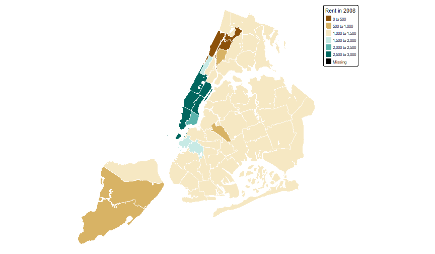<!-- --> ] --- count: false ## Choropleth maps with sf and tmap: NYC examples .panel1-nyc3-auto[ ``` r tm_shape(nyc_shp) + tm_polygons( col = "rent2008", palette = "BrBG", border.col = "white", title = "Rent in 2008" ) + tm_layout(frame = FALSE) -> * rentNYC ``` ] .panel2-nyc3-auto[ ] <style> .panel1-nyc3-auto { color: black; width: 39.2%; hight: 32%; float: left; padding-left: 1%; font-size: 80% } .panel2-nyc3-auto { color: black; width: 58.8%; hight: 32%; float: left; padding-left: 1%; font-size: 80% } .panel3-nyc3-auto { color: black; width: NA%; hight: 33%; float: left; padding-left: 1%; font-size: 80% } </style> --- count: false ## Choropleth maps with sf and tmap: NYC examples .panel1-nyc4-auto[ ``` r *tm_shape(nyc_shp) + tm_polygons( * col = "forhis08", * border.col = "white", * title = "Hispanic population in 2008 (%)" * ) ``` ] .panel2-nyc4-auto[ 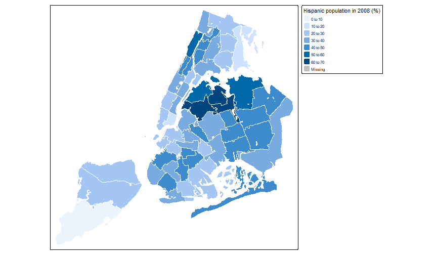<!-- --> ] --- count: false ## Choropleth maps with sf and tmap: NYC examples .panel1-nyc4-auto[ ``` r tm_shape(nyc_shp) + tm_polygons( col = "forhis08", border.col = "white", title = "Hispanic population in 2008 (%)" ) + * tm_layout(frame = FALSE) ``` ] .panel2-nyc4-auto[ 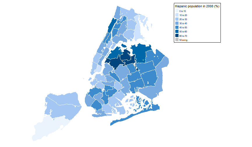<!-- --> ] --- count: false ## Choropleth maps with sf and tmap: NYC examples .panel1-nyc4-auto[ ``` r tm_shape(nyc_shp) + tm_polygons( col = "forhis08", border.col = "white", title = "Hispanic population in 2008 (%)" ) + tm_layout(frame = FALSE) -> * hisNYC ``` ] .panel2-nyc4-auto[ ] <style> .panel1-nyc4-auto { color: black; width: 39.2%; hight: 32%; float: left; padding-left: 1%; font-size: 80% } .panel2-nyc4-auto { color: black; width: 58.8%; hight: 32%; float: left; padding-left: 1%; font-size: 80% } .panel3-nyc4-auto { color: black; width: NA%; hight: 33%; float: left; padding-left: 1%; font-size: 80% } </style> --- count: false ## Choropleth maps with sf and tmap: NYC examples .panel1-nyc5-auto[ ``` r *tm_shape(nyc_shp) + tm_polygons( * col = "pubast00", * palette = "Blues", * border.col = "white", * title = "% of households receiving \nassistance in 2000" * ) ``` ] .panel2-nyc5-auto[ 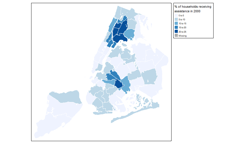<!-- --> ] --- count: false ## Choropleth maps with sf and tmap: NYC examples .panel1-nyc5-auto[ ``` r tm_shape(nyc_shp) + tm_polygons( col = "pubast00", palette = "Blues", border.col = "white", title = "% of households receiving \nassistance in 2000" ) + * tm_layout(frame = FALSE) ``` ] .panel2-nyc5-auto[ 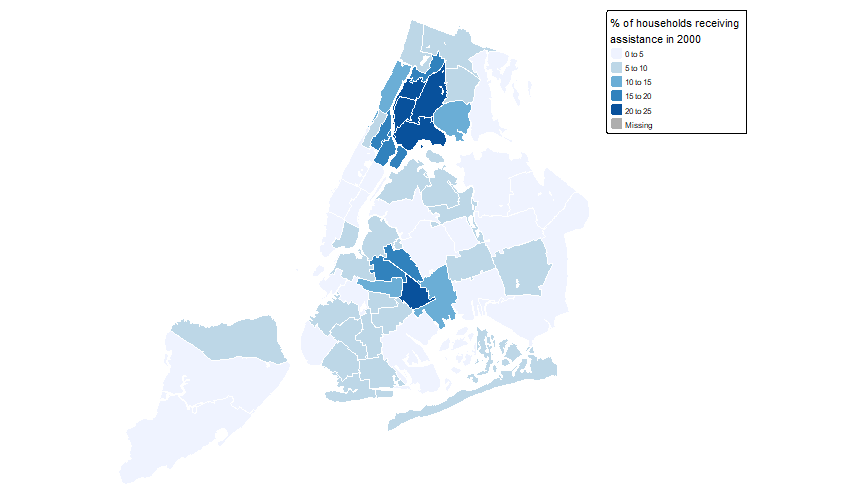<!-- --> ] --- count: false ## Choropleth maps with sf and tmap: NYC examples .panel1-nyc5-auto[ ``` r tm_shape(nyc_shp) + tm_polygons( col = "pubast00", palette = "Blues", border.col = "white", title = "% of households receiving \nassistance in 2000" ) + tm_layout(frame = FALSE) -> * pubastNYC ``` ] .panel2-nyc5-auto[ ] <style> .panel1-nyc5-auto { color: black; width: 39.2%; hight: 32%; float: left; padding-left: 1%; font-size: 80% } .panel2-nyc5-auto { color: black; width: 58.8%; hight: 32%; float: left; padding-left: 1%; font-size: 80% } .panel3-nyc5-auto { color: black; width: NA%; hight: 33%; float: left; padding-left: 1%; font-size: 80% } </style> --- ## Choropleth maps with sf and tmap: NYC examples ``` r tmap_arrange(rentNYC, hisNYC, pubastNYC, nrow = 1) ``` <img src="Lab6_slides_files/figure-html/unnamed-chunk-14-1.png" style="display: block; margin: auto;" /> --- count: false ## Choropleth maps with sf and tmap: NYC examples .panel1-nyc6-auto[ ``` r ## categorize hispanic pop levels *labels <- c("Low hisp pop", * "Mid hisp pop", * "High hisp pop") ``` ] .panel2-nyc6-auto[ ] --- count: false ## Choropleth maps with sf and tmap: NYC examples .panel1-nyc6-auto[ ``` r ## categorize hispanic pop levels labels <- c("Low hisp pop", "Mid hisp pop", "High hisp pop") *nyc_shp ``` ] .panel2-nyc6-auto[ ``` Simple feature collection with 55 features and 34 fields Geometry type: MULTIPOLYGON Dimension: XY Bounding box: xmin: 913037.2 ymin: 120117 xmax: 1067549 ymax: 272751.4 Projected CRS: NAD83 / New York Long Island (ftUS) First 10 features: bor_subb name code subborough forhis06 1 501 North Shore 501 North Shore 37.0657 2 502 Mid-Island 502 Mid-Island 27.9822 3 503 South Shore 503 South Shore 10.7019 4 401 Astoria 401 Astoria 52.0961 5 402 Sunnyside / Woodside 402 Sunnyside/Woodside 62.7242 6 403 Jackson Heights 403 Jackson Heights 68.4834 7 404 Elmhurst / Corona 404 Elmhurst/Corona 69.5219 8 405 Middle Village / Ridgewood 405 Middle Village/Ridgewood 39.4185 9 406 Forest Hills / Rego Park 406 Rego Park/Forest Hills 58.5388 10 407 Flushing / Whitestone 407 Flushing/Whitestone 59.4432 forhis07 forhis08 forhis09 forwh06 forwh07 forwh08 forwh09 hhsiz1990 hhsiz00 1 34.0317 27.3767 29.3091 13.2540 11.8768 11.1788 11.1459 2.7146 2.7338 2 18.1193 24.0452 31.1566 20.0616 19.8575 22.4870 17.0371 2.8233 2.7176 3 12.1404 9.6890 14.6638 10.3060 12.7699 9.3561 10.2830 3.0547 2.8497 4 53.9585 54.6968 47.8050 38.3658 35.6551 32.1289 34.6578 2.4279 2.4995 5 69.3969 67.0897 58.2963 37.0512 31.9057 32.3264 33.8794 2.4646 2.6287 6 68.5405 66.5080 69.1580 34.3999 38.2428 38.1470 26.5347 2.8081 3.1650 7 66.8795 69.3414 64.3005 40.3935 51.6376 45.9578 48.3542 2.9690 3.1784 8 35.9546 36.2750 35.0181 37.8097 34.0156 33.0695 33.0816 2.5174 2.6606 9 52.6183 42.3878 47.9795 43.7395 47.5873 45.1205 39.8293 2.0631 2.1532 10 53.4747 53.2531 57.9868 26.5802 25.6864 21.3858 23.5204 2.6302 2.6818 hhsiz02 hhsiz05 hhsiz08 kids2000 kids2005 kids2006 kids2007 kids2008 1 2.7412 2.8010 2.6983 39.2995 43.3788 38.4022 41.5213 39.8390 2 2.5405 2.6228 2.5749 36.2234 35.7630 36.9081 37.6798 37.2447 3 2.6525 2.6121 2.6483 39.7362 42.5232 40.3577 40.3797 40.4820 4 2.3032 2.3227 2.2746 28.4592 27.2223 25.2556 24.8911 22.0364 5 2.5300 2.4993 2.4766 29.8808 28.6841 28.1440 26.3675 29.9032 6 2.9108 2.8599 2.8604 41.6335 40.2431 39.3135 37.4414 39.4144 7 2.8740 3.1064 3.2223 41.8224 35.8002 40.2321 44.0976 37.2912 8 2.7540 2.7750 2.7007 35.0385 36.6091 37.7748 37.6190 30.9096 9 2.1504 2.1932 2.1512 21.9464 21.4119 24.2723 23.7545 24.7718 10 2.5351 2.5668 2.5857 31.5298 27.7413 28.5853 28.1564 31.1019 kids2009 rent2002 rent2005 rent2008 rentpct02 rentpct05 rentpct08 pubast90 1 40.3169 800 900 1000 21.1119 24.8073 28.5344 47.32913 2 37.8176 650 800 950 32.3615 27.2584 27.9567 35.18232 3 35.3880 750 775 800 23.0547 20.4146 18.1590 23.89404 4 17.9996 1000 1100 1400 25.6022 26.7685 28.0467 80.53393 5 26.2156 1000 1000 1400 18.8079 22.6752 21.3009 75.51687 6 39.0377 910 1000 1100 34.0156 34.8050 27.1032 66.64228 7 43.3207 896 1001 1300 26.7381 34.3842 28.8255 77.53080 8 35.4524 800 900 1100 41.2035 40.6256 36.2956 59.01702 9 21.9552 1000 1035 1400 11.9766 10.4943 11.5520 64.16213 10 28.3184 1000 1100 1200 23.9394 23.3487 22.6715 53.62965 pubast00 yrhom02 yrhom05 yrhom08 geometry 1 6.005791 10.80507 12.127853 11.54743 MULTIPOLYGON (((962498.9 17... 2 2.287034 15.24125 15.183111 14.68212 MULTIPOLYGON (((928296.9 16... 3 1.350208 12.70425 12.972280 13.56149 MULTIPOLYGON (((932416.3 14... 4 5.204510 12.83917 13.377513 12.54464 MULTIPOLYGON (((1010873 226... 5 2.974139 15.38766 12.518789 12.66691 MULTIPOLYGON (((1011647 216... 6 5.332569 12.64923 12.580355 11.96598 MULTIPOLYGON (((1014790 220... 7 6.029230 11.55498 9.828084 10.73805 MULTIPOLYGON (((1018353 205... 8 3.951290 13.49841 12.616178 11.19165 MULTIPOLYGON (((1013477 206... 9 3.111417 13.40156 13.375477 12.74230 MULTIPOLYGON (((1026974 207... 10 2.795721 14.01126 12.806067 12.84800 MULTIPOLYGON (((1034251 230... ``` ] --- count: false ## Choropleth maps with sf and tmap: NYC examples .panel1-nyc6-auto[ ``` r ## categorize hispanic pop levels labels <- c("Low hisp pop", "Mid hisp pop", "High hisp pop") nyc_shp %>% * mutate(forhis08_cat = * cut(forhis08, * breaks = 3, * labels = labels)) ``` ] .panel2-nyc6-auto[ ``` Simple feature collection with 55 features and 35 fields Geometry type: MULTIPOLYGON Dimension: XY Bounding box: xmin: 913037.2 ymin: 120117 xmax: 1067549 ymax: 272751.4 Projected CRS: NAD83 / New York Long Island (ftUS) First 10 features: bor_subb name code subborough forhis06 1 501 North Shore 501 North Shore 37.0657 2 502 Mid-Island 502 Mid-Island 27.9822 3 503 South Shore 503 South Shore 10.7019 4 401 Astoria 401 Astoria 52.0961 5 402 Sunnyside / Woodside 402 Sunnyside/Woodside 62.7242 6 403 Jackson Heights 403 Jackson Heights 68.4834 7 404 Elmhurst / Corona 404 Elmhurst/Corona 69.5219 8 405 Middle Village / Ridgewood 405 Middle Village/Ridgewood 39.4185 9 406 Forest Hills / Rego Park 406 Rego Park/Forest Hills 58.5388 10 407 Flushing / Whitestone 407 Flushing/Whitestone 59.4432 forhis07 forhis08 forhis09 forwh06 forwh07 forwh08 forwh09 hhsiz1990 hhsiz00 1 34.0317 27.3767 29.3091 13.2540 11.8768 11.1788 11.1459 2.7146 2.7338 2 18.1193 24.0452 31.1566 20.0616 19.8575 22.4870 17.0371 2.8233 2.7176 3 12.1404 9.6890 14.6638 10.3060 12.7699 9.3561 10.2830 3.0547 2.8497 4 53.9585 54.6968 47.8050 38.3658 35.6551 32.1289 34.6578 2.4279 2.4995 5 69.3969 67.0897 58.2963 37.0512 31.9057 32.3264 33.8794 2.4646 2.6287 6 68.5405 66.5080 69.1580 34.3999 38.2428 38.1470 26.5347 2.8081 3.1650 7 66.8795 69.3414 64.3005 40.3935 51.6376 45.9578 48.3542 2.9690 3.1784 8 35.9546 36.2750 35.0181 37.8097 34.0156 33.0695 33.0816 2.5174 2.6606 9 52.6183 42.3878 47.9795 43.7395 47.5873 45.1205 39.8293 2.0631 2.1532 10 53.4747 53.2531 57.9868 26.5802 25.6864 21.3858 23.5204 2.6302 2.6818 hhsiz02 hhsiz05 hhsiz08 kids2000 kids2005 kids2006 kids2007 kids2008 1 2.7412 2.8010 2.6983 39.2995 43.3788 38.4022 41.5213 39.8390 2 2.5405 2.6228 2.5749 36.2234 35.7630 36.9081 37.6798 37.2447 3 2.6525 2.6121 2.6483 39.7362 42.5232 40.3577 40.3797 40.4820 4 2.3032 2.3227 2.2746 28.4592 27.2223 25.2556 24.8911 22.0364 5 2.5300 2.4993 2.4766 29.8808 28.6841 28.1440 26.3675 29.9032 6 2.9108 2.8599 2.8604 41.6335 40.2431 39.3135 37.4414 39.4144 7 2.8740 3.1064 3.2223 41.8224 35.8002 40.2321 44.0976 37.2912 8 2.7540 2.7750 2.7007 35.0385 36.6091 37.7748 37.6190 30.9096 9 2.1504 2.1932 2.1512 21.9464 21.4119 24.2723 23.7545 24.7718 10 2.5351 2.5668 2.5857 31.5298 27.7413 28.5853 28.1564 31.1019 kids2009 rent2002 rent2005 rent2008 rentpct02 rentpct05 rentpct08 pubast90 1 40.3169 800 900 1000 21.1119 24.8073 28.5344 47.32913 2 37.8176 650 800 950 32.3615 27.2584 27.9567 35.18232 3 35.3880 750 775 800 23.0547 20.4146 18.1590 23.89404 4 17.9996 1000 1100 1400 25.6022 26.7685 28.0467 80.53393 5 26.2156 1000 1000 1400 18.8079 22.6752 21.3009 75.51687 6 39.0377 910 1000 1100 34.0156 34.8050 27.1032 66.64228 7 43.3207 896 1001 1300 26.7381 34.3842 28.8255 77.53080 8 35.4524 800 900 1100 41.2035 40.6256 36.2956 59.01702 9 21.9552 1000 1035 1400 11.9766 10.4943 11.5520 64.16213 10 28.3184 1000 1100 1200 23.9394 23.3487 22.6715 53.62965 pubast00 yrhom02 yrhom05 yrhom08 geometry 1 6.005791 10.80507 12.127853 11.54743 MULTIPOLYGON (((962498.9 17... 2 2.287034 15.24125 15.183111 14.68212 MULTIPOLYGON (((928296.9 16... 3 1.350208 12.70425 12.972280 13.56149 MULTIPOLYGON (((932416.3 14... 4 5.204510 12.83917 13.377513 12.54464 MULTIPOLYGON (((1010873 226... 5 2.974139 15.38766 12.518789 12.66691 MULTIPOLYGON (((1011647 216... 6 5.332569 12.64923 12.580355 11.96598 MULTIPOLYGON (((1014790 220... 7 6.029230 11.55498 9.828084 10.73805 MULTIPOLYGON (((1018353 205... 8 3.951290 13.49841 12.616178 11.19165 MULTIPOLYGON (((1013477 206... 9 3.111417 13.40156 13.375477 12.74230 MULTIPOLYGON (((1026974 207... 10 2.795721 14.01126 12.806067 12.84800 MULTIPOLYGON (((1034251 230... forhis08_cat 1 Low hisp pop 2 Low hisp pop 3 Low hisp pop 4 High hisp pop 5 High hisp pop 6 High hisp pop 7 High hisp pop 8 Mid hisp pop 9 Mid hisp pop 10 High hisp pop ``` ] --- count: false ## Choropleth maps with sf and tmap: NYC examples .panel1-nyc6-auto[ ``` r ## categorize hispanic pop levels labels <- c("Low hisp pop", "Mid hisp pop", "High hisp pop") nyc_shp %>% mutate(forhis08_cat = cut(forhis08, breaks = 3, labels = labels)) -> * nyc_shp2 ``` ] .panel2-nyc6-auto[ ] <style> .panel1-nyc6-auto { color: black; width: 39.2%; hight: 32%; float: left; padding-left: 1%; font-size: 80% } .panel2-nyc6-auto { color: black; width: 58.8%; hight: 32%; float: left; padding-left: 1%; font-size: 80% } .panel3-nyc6-auto { color: black; width: NA%; hight: 33%; float: left; padding-left: 1%; font-size: 80% } </style> --- count: false ## Choropleth maps with sf and tmap: NYC examples .panel1-nyc7-non_seq[ ``` r tm_shape(nyc_shp2) + tm_polygons( col = "rent2008", palette = "BrBG", border.col = "white", title = "Rent in 2008" ) ``` ] .panel2-nyc7-non_seq[ <!-- --> ] --- count: false ## Choropleth maps with sf and tmap: NYC examples .panel1-nyc7-non_seq[ ``` r tm_shape(nyc_shp2) + tm_polygons( col = "rent2008", palette = "BrBG", border.col = "white", title = "Rent in 2008" ) + * tm_facets( * by = "forhis08_cat", * drop.units = TRUE, * ) ``` ] .panel2-nyc7-non_seq[ 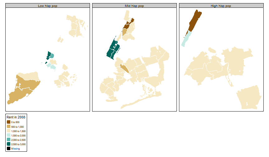<!-- --> ] --- count: false ## Choropleth maps with sf and tmap: NYC examples .panel1-nyc7-non_seq[ ``` r tm_shape(nyc_shp2) + tm_polygons( col = "rent2008", palette = "BrBG", border.col = "white", title = "Rent in 2008" ) + tm_facets( by = "forhis08_cat", drop.units = TRUE, * free.coords = FALSE, ) ``` ] .panel2-nyc7-non_seq[ 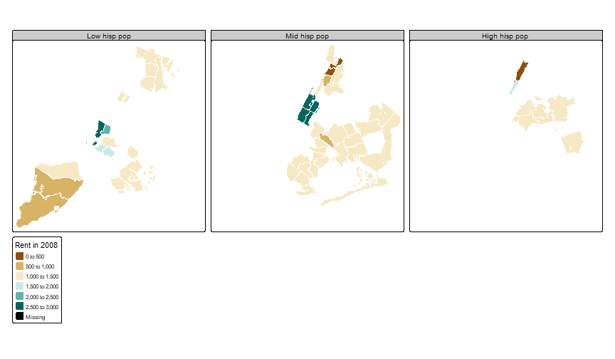<!-- --> ] --- count: false ## Choropleth maps with sf and tmap: NYC examples .panel1-nyc7-non_seq[ ``` r tm_shape(nyc_shp2) + tm_polygons( col = "rent2008", palette = "BrBG", border.col = "white", title = "Rent in 2008" ) + tm_facets( by = "forhis08_cat", drop.units = TRUE, free.coords = FALSE, ) + * tm_layout( * legend.outside.size = 0.135, * ) ``` ] .panel2-nyc7-non_seq[ <!-- --> ] --- count: false ## Choropleth maps with sf and tmap: NYC examples .panel1-nyc7-non_seq[ ``` r tm_shape(nyc_shp2) + tm_polygons( col = "rent2008", palette = "BrBG", border.col = "white", title = "Rent in 2008" ) + tm_facets( by = "forhis08_cat", drop.units = TRUE, free.coords = FALSE, ) + tm_layout( legend.outside.size = 0.135, * frame = FALSE, ) ``` ] .panel2-nyc7-non_seq[ 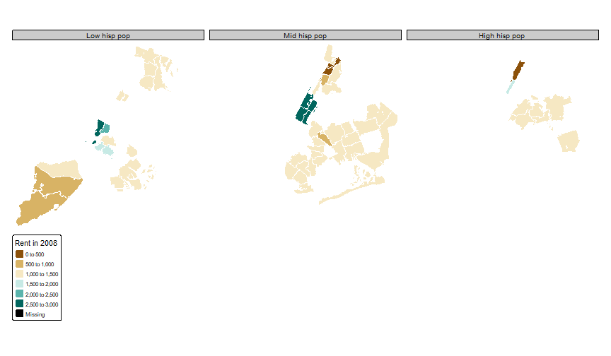<!-- --> ] --- count: false ## Choropleth maps with sf and tmap: NYC examples .panel1-nyc7-non_seq[ ``` r tm_shape(nyc_shp2) + tm_polygons( col = "rent2008", palette = "BrBG", border.col = "white", title = "Rent in 2008" ) + tm_facets( by = "forhis08_cat", drop.units = TRUE, free.coords = FALSE, ) + tm_layout( legend.outside.size = 0.135, frame = FALSE, * panel.label.bg.color = NA, ) ``` ] .panel2-nyc7-non_seq[ <!-- --> ] --- count: false ## Choropleth maps with sf and tmap: NYC examples .panel1-nyc7-non_seq[ ``` r tm_shape(nyc_shp2) + tm_polygons( col = "rent2008", palette = "BrBG", border.col = "white", title = "Rent in 2008" ) + tm_facets( by = "forhis08_cat", drop.units = TRUE, free.coords = FALSE, ) + tm_layout( legend.outside.size = 0.135, frame = FALSE, panel.label.bg.color = NA, * frame.lwd = 0, ) ``` ] .panel2-nyc7-non_seq[ <!-- --> ] --- count: false ## Choropleth maps with sf and tmap: NYC examples .panel1-nyc7-non_seq[ ``` r tm_shape(nyc_shp2) + tm_polygons( col = "rent2008", palette = "BrBG", border.col = "white", title = "Rent in 2008" ) + tm_facets( by = "forhis08_cat", drop.units = TRUE, free.coords = FALSE, ) + tm_layout( legend.outside.size = 0.135, frame = FALSE, panel.label.bg.color = NA, frame.lwd = 0, * panel.label.size = 1.5 ) ``` ] .panel2-nyc7-non_seq[ 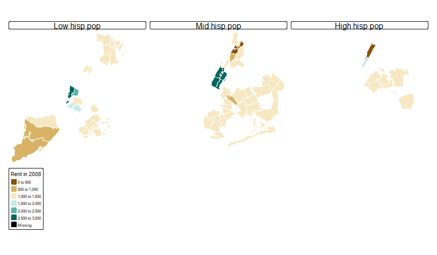<!-- --> ] --- count: false ## Choropleth maps with sf and tmap: NYC examples .panel1-nyc7-non_seq[ ``` r tm_shape(nyc_shp2) + tm_polygons( col = "rent2008", palette = "BrBG", border.col = "white", title = "Rent in 2008" ) + tm_facets( by = "forhis08_cat", drop.units = TRUE, free.coords = FALSE, ) + tm_layout( legend.outside.size = 0.135, frame = FALSE, panel.label.bg.color = NA, frame.lwd = 0, panel.label.size = 1.5 ) + * tm_shape(nyc_shp2) + * tm_borders(col = "grey75", lty = 2) ``` ] .panel2-nyc7-non_seq[ 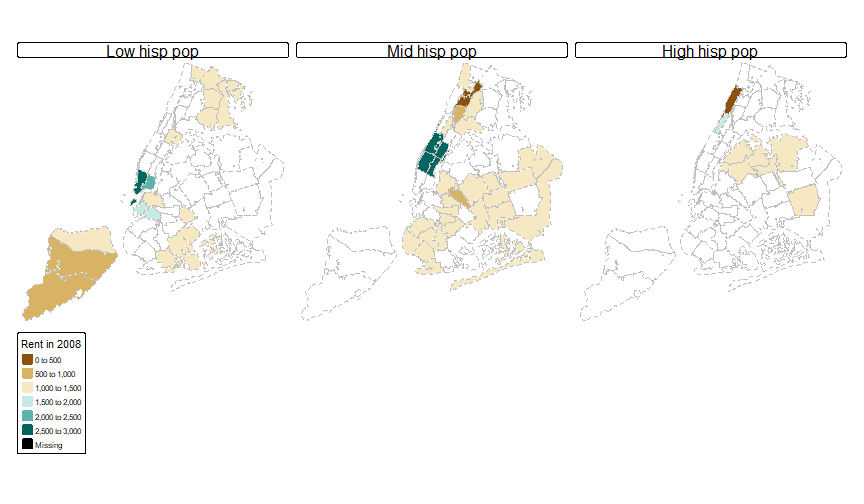<!-- --> ] <style> .panel1-nyc7-non_seq { color: black; width: 39.2%; hight: 32%; float: left; padding-left: 1%; font-size: 80% } .panel2-nyc7-non_seq { color: black; width: 58.8%; hight: 32%; float: left; padding-left: 1%; font-size: 80% } .panel3-nyc7-non_seq { color: black; width: NA%; hight: 33%; float: left; padding-left: 1%; font-size: 80% } </style>