class: center, middle, inverse, title-slide .title[ # CS&SS 569 Visualizing Data and Models ] .subtitle[ ## Lab 7: Visualizing relational data ] .author[ ### Brian Leung ] .institute[ ### Department of Political Science, UW ] .date[ ### 2023-02-17 ] --- ## Introduction - Cover different ways to visualize network or relational data -- - Node-edge diagram (classic network visualization) with **`tidygraph`** and **`ggraph`** -- - Heat map (plus cluster analysis) with **`ggplot2`** and **`cluster`** -- - Increasingly popular ways -- - Chord diagram with **`circlize`** -- - Sankey diagrams with **`ggsankey`** (or alluvial diagram with **`ggalluvial`**) --- ## Network visualization - Map of sciences (Bollen et al. 2009) based on clickstream data on journal websites <img src="figures/journal.pone.0004803.g005.png" width="32.5%" style="display: block; margin: auto;" /> --- ## Challenges - Network data create many challenges for visualization -- - Cursed by high dimensionality -- - Network diagrams usually result in hairballs or spaghetti balls. . . -- - One takeaway from this lab is to take advantage of alternative visualization methods when possible -- - Not just network data, but more generically, *relational* data -- - Any data whose unit of observation is dyadic -- - E.g., migration flow data, or import/export data, between a pair of countries --- ## Examples in class - Florentine families and the rise of Medici: node-edge diagram <img src="figures/medici.png" width="65%" style="display: block; margin: auto;" /> --- ## Examples in class - Migration flow data: heat map with cluster analysis <img src="figures/migrat_heatmap.png" width="32.5%" style="display: block; margin: auto;" /> --- ## Examples in class - Migration flow data: chord diagram <img src="figures/migrat_chord.png" width="32.5%" style="display: block; margin: auto;" /> --- ## Examples in class - Migration flow data: sankey diagram <img src="figures/migrat_sankey.png" width="32.5%" style="display: block; margin: auto;" /> --- ## Prerequisite ```r # download packages packages <- c("tidyverse", "tidygraph", "ggraph", "reshape2", "cluster", "circlize") not_installed <- setdiff(packages, rownames(installed.packages())) if (length(not_installed)) install.packages(not_installed) # install developmental version of ggsankey devtools::install_github("davidsjoberg/ggsankey") # load packages library(tidyverse) library(tidygraph) library(ggraph) library(reshape2) library(cluster) library(circlize) library(ggsankey) ``` --- count: false ## Rise of Medici: Adjacency Matrix .panel1-medici1-auto[ ```r # load data *medici <- read.table("data/medici.txt") ``` ] .panel2-medici1-auto[ ] --- count: false ## Rise of Medici: Adjacency Matrix .panel1-medici1-auto[ ```r # load data medici <- read.table("data/medici.txt") # examine the data *head(medici) ``` ] .panel2-medici1-auto[ ``` Acciaiuoli Albizzi Barbadori Bischeri Castellani Ginori Guadagni Acciaiuoli 0 0 0 0 0 0 0 Albizzi 0 0 0 0 0 1 1 Barbadori 0 0 0 0 1 0 0 Bischeri 0 0 0 0 0 0 1 Castellani 0 0 1 0 0 0 0 Ginori 0 1 0 0 0 0 0 Lamberteschi Medici Pazzi Peruzzi Pucci Ridolfi Salviati Strozzi Acciaiuoli 0 1 0 0 0 0 0 0 Albizzi 0 1 0 0 0 0 0 0 Barbadori 0 1 0 0 0 0 0 0 Bischeri 0 0 0 1 0 0 0 1 Castellani 0 0 0 1 0 0 0 1 Ginori 0 0 0 0 0 0 0 0 Tornabuoni Acciaiuoli 0 Albizzi 0 Barbadori 0 Bischeri 0 Castellani 0 Ginori 0 ``` ] <style> .panel1-medici1-auto { color: black; width: 49%; hight: 32%; float: left; padding-left: 1%; font-size: 80% } .panel2-medici1-auto { color: black; width: 49%; hight: 32%; float: left; padding-left: 1%; font-size: 80% } .panel3-medici1-auto { color: black; width: NA%; hight: 33%; float: left; padding-left: 1%; font-size: 80% } </style> --- count: false ## Rise of Medici: tidygraph package for manipulation .panel1-medici2-auto[ ```r # coerce into a tbl_graph using tidygraph *medici_graph <- as_tbl_graph(medici, directed = FALSE) ``` ] .panel2-medici2-auto[ ] --- count: false ## Rise of Medici: tidygraph package for manipulation .panel1-medici2-auto[ ```r # coerce into a tbl_graph using tidygraph medici_graph <- as_tbl_graph(medici, directed = FALSE) # examine the tbl_graph *medici_graph ``` ] .panel2-medici2-auto[ ``` # A tbl_graph: 16 nodes and 58 edges # # An undirected multigraph with 2 components # # Node Data: 16 × 1 (active) name <chr> 1 Acciaiuoli 2 Albizzi 3 Barbadori 4 Bischeri 5 Castellani 6 Ginori # … with 10 more rows # # Edge Data: 58 × 3 from to weight <int> <int> <dbl> 1 1 1 1 2 1 2 1 3 1 3 1 # … with 55 more rows ``` ] <style> .panel1-medici2-auto { color: black; width: 49%; hight: 32%; float: left; padding-left: 1%; font-size: 80% } .panel2-medici2-auto { color: black; width: 49%; hight: 32%; float: left; padding-left: 1%; font-size: 80% } .panel3-medici2-auto { color: black; width: NA%; hight: 33%; float: left; padding-left: 1%; font-size: 80% } </style> --- count: false ## Rise of Medici: Basic visualization w/ ggraph .panel1-medici3-auto[ ```r *ggraph(medici_graph) ``` ] .panel2-medici3-auto[ <!-- --> ] --- count: false ## Rise of Medici: Basic visualization w/ ggraph .panel1-medici3-auto[ ```r ggraph(medici_graph) + * geom_node_point() ``` ] .panel2-medici3-auto[ <!-- --> ] --- count: false ## Rise of Medici: Basic visualization w/ ggraph .panel1-medici3-auto[ ```r ggraph(medici_graph) + geom_node_point() + * geom_edge_link() ``` ] .panel2-medici3-auto[ <!-- --> ] --- count: false ## Rise of Medici: Basic visualization w/ ggraph .panel1-medici3-auto[ ```r ggraph(medici_graph) + geom_node_point() + geom_edge_link() + * geom_node_text(aes(label = name), repel = TRUE) ``` ] .panel2-medici3-auto[ <!-- --> ] --- count: false ## Rise of Medici: Basic visualization w/ ggraph .panel1-medici3-auto[ ```r ggraph(medici_graph) + geom_node_point() + geom_edge_link() + geom_node_text(aes(label = name), repel = TRUE) + * theme_graph() ``` ] .panel2-medici3-auto[ <!-- --> ] <style> .panel1-medici3-auto { color: black; width: 49%; hight: 32%; float: left; padding-left: 1%; font-size: 80% } .panel2-medici3-auto { color: black; width: 49%; hight: 32%; float: left; padding-left: 1%; font-size: 80% } .panel3-medici3-auto { color: black; width: NA%; hight: 33%; float: left; padding-left: 1%; font-size: 80% } </style> --- count: false ## Rise of Medici: tidygraph package for network computation .panel1-medici4-auto[ ```r *medici_graph ``` ] .panel2-medici4-auto[ ``` # A tbl_graph: 16 nodes and 58 edges # # An undirected multigraph with 2 components # # Node Data: 16 × 1 (active) name <chr> 1 Acciaiuoli 2 Albizzi 3 Barbadori 4 Bischeri 5 Castellani 6 Ginori # … with 10 more rows # # Edge Data: 58 × 3 from to weight <int> <int> <dbl> 1 1 1 1 2 1 2 1 3 1 3 1 # … with 55 more rows ``` ] --- count: false ## Rise of Medici: tidygraph package for network computation .panel1-medici4-auto[ ```r medici_graph %>% * mutate( * degree = centrality_degree(), # degree centrality * community = group_leading_eigen() # community-detection algorithm * ) ``` ] .panel2-medici4-auto[ ``` # A tbl_graph: 16 nodes and 58 edges # # An undirected multigraph with 2 components # # Node Data: 16 × 3 (active) name degree community <chr> <dbl> <int> 1 Acciaiuoli 7 1 2 Albizzi 9 1 3 Barbadori 9 1 4 Bischeri 9 2 5 Castellani 7 2 6 Ginori 4 3 # … with 10 more rows # # Edge Data: 58 × 3 from to weight <int> <int> <dbl> 1 1 1 1 2 1 2 1 3 1 3 1 # … with 55 more rows ``` ] --- count: false ## Rise of Medici: tidygraph package for network computation .panel1-medici4-auto[ ```r medici_graph %>% mutate( degree = centrality_degree(), # degree centrality community = group_leading_eigen() # community-detection algorithm ) -> * medici_graph ``` ] .panel2-medici4-auto[ ] <style> .panel1-medici4-auto { color: black; width: 49%; hight: 32%; float: left; padding-left: 1%; font-size: 80% } .panel2-medici4-auto { color: black; width: 49%; hight: 32%; float: left; padding-left: 1%; font-size: 80% } .panel3-medici4-auto { color: black; width: NA%; hight: 33%; float: left; padding-left: 1%; font-size: 80% } </style> --- count: false ## Rise of Medici: Basic visualization w/ ggraph .panel1-medici5-non_seq[ ```r ggraph( medici_graph, ) ``` ] .panel2-medici5-non_seq[ <!-- --> ] --- count: false ## Rise of Medici: Basic visualization w/ ggraph .panel1-medici5-non_seq[ ```r ggraph( medici_graph, ) + * geom_edge_link(alpha = 0.5) ``` ] .panel2-medici5-non_seq[ <!-- --> ] --- count: false ## Rise of Medici: Basic visualization w/ ggraph .panel1-medici5-non_seq[ ```r ggraph( medici_graph, ) + geom_edge_link(alpha = 0.5) + * geom_node_point(aes(size = degree, * )) ``` ] .panel2-medici5-non_seq[ <!-- --> ] --- count: false ## Rise of Medici: Basic visualization w/ ggraph .panel1-medici5-non_seq[ ```r ggraph( medici_graph, ) + geom_edge_link(alpha = 0.5) + geom_node_point(aes(size = degree, * color = factor(community) )) ``` ] .panel2-medici5-non_seq[ <!-- --> ] --- count: false ## Rise of Medici: Basic visualization w/ ggraph .panel1-medici5-non_seq[ ```r ggraph( medici_graph, ) + geom_edge_link(alpha = 0.5) + geom_node_point(aes(size = degree, color = factor(community) )) + * geom_node_text(aes(label = name, * ), * repel = TRUE) ``` ] .panel2-medici5-non_seq[ <!-- --> ] --- count: false ## Rise of Medici: Basic visualization w/ ggraph .panel1-medici5-non_seq[ ```r ggraph( medici_graph, ) + geom_edge_link(alpha = 0.5) + geom_node_point(aes(size = degree, color = factor(community) )) + geom_node_text(aes(label = name, * size = degree ), repel = TRUE) ``` ] .panel2-medici5-non_seq[ 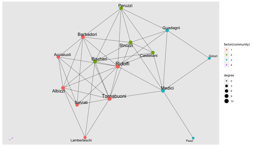<!-- --> ] --- count: false ## Rise of Medici: Basic visualization w/ ggraph .panel1-medici5-non_seq[ ```r ggraph( medici_graph, ) + geom_edge_link(alpha = 0.5) + geom_node_point(aes(size = degree, color = factor(community) )) + geom_node_text(aes(label = name, size = degree ), repel = TRUE) + * scale_color_brewer(palette = "Set1") ``` ] .panel2-medici5-non_seq[ 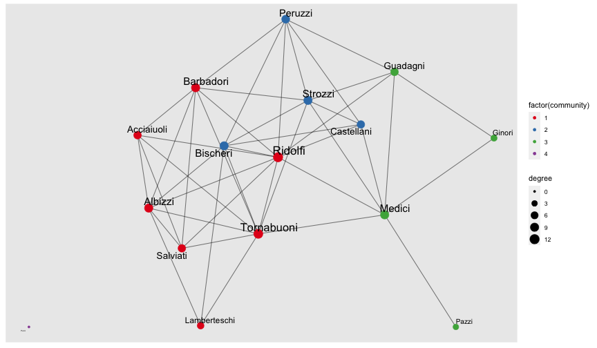<!-- --> ] --- count: false ## Rise of Medici: Basic visualization w/ ggraph .panel1-medici5-non_seq[ ```r ggraph( medici_graph, ) + geom_edge_link(alpha = 0.5) + geom_node_point(aes(size = degree, color = factor(community) )) + geom_node_text(aes(label = name, size = degree ), repel = TRUE) + scale_color_brewer(palette = "Set1") + * theme_graph() + theme(legend.position = "none") ``` ] .panel2-medici5-non_seq[ 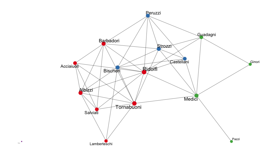<!-- --> ] --- count: false ## Rise of Medici: Basic visualization w/ ggraph .panel1-medici5-non_seq[ ```r ggraph( medici_graph, * layout = "circle" ) + geom_edge_link(alpha = 0.5) + geom_node_point(aes(size = degree, color = factor(community) )) + geom_node_text(aes(label = name, size = degree ), repel = TRUE) + scale_color_brewer(palette = "Set1") + theme_graph() + theme(legend.position = "none") ``` ] .panel2-medici5-non_seq[ 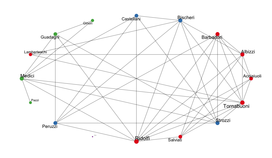<!-- --> ] <style> .panel1-medici5-non_seq { color: black; width: 49%; hight: 32%; float: left; padding-left: 1%; font-size: 80% } .panel2-medici5-non_seq { color: black; width: 49%; hight: 32%; float: left; padding-left: 1%; font-size: 80% } .panel3-medici5-non_seq { color: black; width: NA%; hight: 33%; float: left; padding-left: 1%; font-size: 80% } </style> --- ## Alternative tools for making node-edge diagram - Check out [Gephi](https://gephi.org/), a free and open-source tool for network visualization -- - Suitable for large-N, complex networks -- - From [Martin Grandjean](https://www.martingrandjean.ch/intellectual-cooperation-multi-level-network-analysis/) <img src="figures/IntellectualCooperationMultiLevel.png" width="42.5%" style="display: block; margin: auto;" /> --- count: false ## Migration flow: node-edge diagram? .panel1-migrat1-auto[ ```r # load data *migrat2010 <- read_csv("data/migrat2010.csv") ``` ] .panel2-migrat1-auto[ ] --- count: false ## Migration flow: node-edge diagram? .panel1-migrat1-auto[ ```r # load data migrat2010 <- read_csv("data/migrat2010.csv") # examine data: long list instead of adjacency matrix *print(migrat2010) ``` ] .panel2-migrat1-auto[ ``` # A tibble: 212 × 3 origRegion destRegion flow <chr> <chr> <dbl> 1 Caribbean Caribbean 40506 2 Caribbean Central America 8183 3 Caribbean Northern America 533052 4 Caribbean Northern Europe 15584 5 Caribbean South America 3264 6 Caribbean Southern Europe 21711 7 Caribbean Western Europe 14875 8 Central America Central America 99171 9 Central America Northern America 1262880 10 Central America Northern Europe 1136 # … with 202 more rows ``` ] --- count: false ## Migration flow: node-edge diagram? .panel1-migrat1-auto[ ```r # load data migrat2010 <- read_csv("data/migrat2010.csv") # examine data: long list instead of adjacency matrix print(migrat2010) # coerce to tbl_graph *migrat2010_graph <- as_tbl_graph(migrat2010) ``` ] .panel2-migrat1-auto[ ``` # A tibble: 212 × 3 origRegion destRegion flow <chr> <chr> <dbl> 1 Caribbean Caribbean 40506 2 Caribbean Central America 8183 3 Caribbean Northern America 533052 4 Caribbean Northern Europe 15584 5 Caribbean South America 3264 6 Caribbean Southern Europe 21711 7 Caribbean Western Europe 14875 8 Central America Central America 99171 9 Central America Northern America 1262880 10 Central America Northern Europe 1136 # … with 202 more rows ``` ] <style> .panel1-migrat1-auto { color: black; width: 49%; hight: 32%; float: left; padding-left: 1%; font-size: 80% } .panel2-migrat1-auto { color: black; width: 49%; hight: 32%; float: left; padding-left: 1%; font-size: 80% } .panel3-migrat1-auto { color: black; width: NA%; hight: 33%; float: left; padding-left: 1%; font-size: 80% } </style> --- count: false ## Migration flow: node-edge diagram? .panel1-migrat2-non_seq[ ```r ggraph(migrat2010_graph) ``` ] .panel2-migrat2-non_seq[ <!-- --> ] --- count: false ## Migration flow: node-edge diagram? .panel1-migrat2-non_seq[ ```r ggraph(migrat2010_graph) + * geom_edge_link( * alpha = 0.5, * ) ``` ] .panel2-migrat2-non_seq[ <!-- --> ] --- count: false ## Migration flow: node-edge diagram? .panel1-migrat2-non_seq[ ```r ggraph(migrat2010_graph) + geom_edge_link( alpha = 0.5, ) + * geom_node_point() ``` ] .panel2-migrat2-non_seq[ <!-- --> ] --- count: false ## Migration flow: node-edge diagram? .panel1-migrat2-non_seq[ ```r ggraph(migrat2010_graph) + geom_edge_link( alpha = 0.5, ) + geom_node_point() + * geom_node_text(aes(label = name), repel = TRUE) ``` ] .panel2-migrat2-non_seq[ <!-- --> ] --- count: false ## Migration flow: node-edge diagram? .panel1-migrat2-non_seq[ ```r ggraph(migrat2010_graph) + geom_edge_link( alpha = 0.5, ) + geom_node_point() + geom_node_text(aes(label = name), repel = TRUE) + * theme_graph() ``` ] .panel2-migrat2-non_seq[ <!-- --> ] --- count: false ## Migration flow: node-edge diagram? .panel1-migrat2-non_seq[ ```r ggraph(migrat2010_graph) + geom_edge_link( alpha = 0.5, * start_cap = circle(2.5, 'mm'), ) + geom_node_point() + geom_node_text(aes(label = name), repel = TRUE) + theme_graph() ``` ] .panel2-migrat2-non_seq[ <!-- --> ] --- count: false ## Migration flow: node-edge diagram? .panel1-migrat2-non_seq[ ```r ggraph(migrat2010_graph) + geom_edge_link( alpha = 0.5, start_cap = circle(2.5, 'mm'), * end_cap = circle(2.5, 'mm'), ) + geom_node_point() + geom_node_text(aes(label = name), repel = TRUE) + theme_graph() ``` ] .panel2-migrat2-non_seq[ <!-- --> ] --- count: false ## Migration flow: node-edge diagram? .panel1-migrat2-non_seq[ ```r ggraph(migrat2010_graph) + geom_edge_link( alpha = 0.5, start_cap = circle(2.5, 'mm'), end_cap = circle(2.5, 'mm'), * arrow = arrow(length = unit(2.5, 'mm')) ) + geom_node_point() + geom_node_text(aes(label = name), repel = TRUE) + theme_graph() ``` ] .panel2-migrat2-non_seq[ <!-- --> ] <style> .panel1-migrat2-non_seq { color: black; width: 49%; hight: 32%; float: left; padding-left: 1%; font-size: 80% } .panel2-migrat2-non_seq { color: black; width: 49%; hight: 32%; float: left; padding-left: 1%; font-size: 80% } .panel3-migrat2-non_seq { color: black; width: NA%; hight: 33%; float: left; padding-left: 1%; font-size: 80% } </style> --- count: false ## Migration flow: what about heat map? .panel1-migrat3-auto[ ```r *ggplot(migrat2010, aes(y = origRegion, * x = destRegion, * fill = flow)) ``` ] .panel2-migrat3-auto[ <!-- --> ] --- count: false ## Migration flow: what about heat map? .panel1-migrat3-auto[ ```r ggplot(migrat2010, aes(y = origRegion, x = destRegion, fill = flow)) + * geom_tile(color = "white", size = 0.2) ``` ] .panel2-migrat3-auto[ <!-- --> ] --- count: false ## Migration flow: what about heat map? .panel1-migrat3-auto[ ```r ggplot(migrat2010, aes(y = origRegion, x = destRegion, fill = flow)) + geom_tile(color = "white", size = 0.2) + * coord_equal() ``` ] .panel2-migrat3-auto[ <!-- --> ] --- count: false ## Migration flow: what about heat map? .panel1-migrat3-auto[ ```r ggplot(migrat2010, aes(y = origRegion, x = destRegion, fill = flow)) + geom_tile(color = "white", size = 0.2) + coord_equal() + * theme(panel.background = element_blank()) ``` ] .panel2-migrat3-auto[ <!-- --> ] <style> .panel1-migrat3-auto { color: black; width: 49%; hight: 32%; float: left; padding-left: 1%; font-size: 80% } .panel2-migrat3-auto { color: black; width: 49%; hight: 32%; float: left; padding-left: 1%; font-size: 80% } .panel3-migrat3-auto { color: black; width: NA%; hight: 33%; float: left; padding-left: 1%; font-size: 80% } </style> --- ## Migration flow: improving the heat map - Three wrangling and analytical tasks: - Make NA values explicit - Turn flow into a categorical variable - Implement cluster analysis to sort countries --- count: false ## Migration flow: improving the heat map .panel1-migrat4-auto[ ```r # use expand to create all unique combinations of variables *migrat2010 ``` ] .panel2-migrat4-auto[ ``` # A tibble: 212 × 3 origRegion destRegion flow <chr> <chr> <dbl> 1 Caribbean Caribbean 40506 2 Caribbean Central America 8183 3 Caribbean Northern America 533052 4 Caribbean Northern Europe 15584 5 Caribbean South America 3264 6 Caribbean Southern Europe 21711 7 Caribbean Western Europe 14875 8 Central America Central America 99171 9 Central America Northern America 1262880 10 Central America Northern Europe 1136 # … with 202 more rows ``` ] --- count: false ## Migration flow: improving the heat map .panel1-migrat4-auto[ ```r # use expand to create all unique combinations of variables migrat2010 %>% * expand(origRegion, destRegion) ``` ] .panel2-migrat4-auto[ ``` # A tibble: 361 × 2 origRegion destRegion <chr> <chr> 1 Caribbean Caribbean 2 Caribbean Central America 3 Caribbean Central Asia 4 Caribbean Eastern Africa 5 Caribbean Eastern Asia 6 Caribbean Eastern Europe 7 Caribbean Middle Africa 8 Caribbean Northern Africa 9 Caribbean Northern America 10 Caribbean Northern Europe # … with 351 more rows ``` ] --- count: false ## Migration flow: improving the heat map .panel1-migrat4-auto[ ```r # use expand to create all unique combinations of variables migrat2010 %>% expand(origRegion, destRegion) %>% * left_join(migrat2010, by = c("origRegion", "destRegion")) ``` ] .panel2-migrat4-auto[ ``` # A tibble: 361 × 3 origRegion destRegion flow <chr> <chr> <dbl> 1 Caribbean Caribbean 40506 2 Caribbean Central America 8183 3 Caribbean Central Asia NA 4 Caribbean Eastern Africa NA 5 Caribbean Eastern Asia NA 6 Caribbean Eastern Europe NA 7 Caribbean Middle Africa NA 8 Caribbean Northern Africa NA 9 Caribbean Northern America 533052 10 Caribbean Northern Europe 15584 # … with 351 more rows ``` ] --- count: false ## Migration flow: improving the heat map .panel1-migrat4-auto[ ```r # use expand to create all unique combinations of variables migrat2010 %>% expand(origRegion, destRegion) %>% left_join(migrat2010, by = c("origRegion", "destRegion")) -> * migrat2010 ``` ] .panel2-migrat4-auto[ ] <style> .panel1-migrat4-auto { color: black; width: 49%; hight: 32%; float: left; padding-left: 1%; font-size: 80% } .panel2-migrat4-auto { color: black; width: 49%; hight: 32%; float: left; padding-left: 1%; font-size: 80% } .panel3-migrat4-auto { color: black; width: NA%; hight: 33%; float: left; padding-left: 1%; font-size: 80% } </style> --- count: false ## Migration flow: improving the heat map .panel1-migrat5-auto[ ```r # find appropriate breaks *quantile(migrat2010$flow, na.rm = TRUE) ``` ] .panel2-migrat5-auto[ ``` 0% 25% 50% 75% 100% 1058.00 9147.75 36104.00 153035.50 4497527.00 ``` ] --- count: false ## Migration flow: improving the heat map .panel1-migrat5-auto[ ```r # find appropriate breaks quantile(migrat2010$flow, na.rm = TRUE) *breaks <- c(1000, 5000, 10000, 50000, 100000, Inf) ``` ] .panel2-migrat5-auto[ ``` 0% 25% 50% 75% 100% 1058.00 9147.75 36104.00 153035.50 4497527.00 ``` ] --- count: false ## Migration flow: improving the heat map .panel1-migrat5-auto[ ```r # find appropriate breaks quantile(migrat2010$flow, na.rm = TRUE) breaks <- c(1000, 5000, 10000, 50000, 100000, Inf) *labels <- c("1000-5000", "5000-10000", "10000-50000", * "50000-100000", ">100000") ``` ] .panel2-migrat5-auto[ ``` 0% 25% 50% 75% 100% 1058.00 9147.75 36104.00 153035.50 4497527.00 ``` ] --- count: false ## Migration flow: improving the heat map .panel1-migrat5-auto[ ```r # find appropriate breaks quantile(migrat2010$flow, na.rm = TRUE) breaks <- c(1000, 5000, 10000, 50000, 100000, Inf) labels <- c("1000-5000", "5000-10000", "10000-50000", "50000-100000", ">100000") # coerce flow into factors *migrat2010 ``` ] .panel2-migrat5-auto[ ``` 0% 25% 50% 75% 100% 1058.00 9147.75 36104.00 153035.50 4497527.00 ``` ``` # A tibble: 361 × 3 origRegion destRegion flow <chr> <chr> <dbl> 1 Caribbean Caribbean 40506 2 Caribbean Central America 8183 3 Caribbean Central Asia NA 4 Caribbean Eastern Africa NA 5 Caribbean Eastern Asia NA 6 Caribbean Eastern Europe NA 7 Caribbean Middle Africa NA 8 Caribbean Northern Africa NA 9 Caribbean Northern America 533052 10 Caribbean Northern Europe 15584 # … with 351 more rows ``` ] --- count: false ## Migration flow: improving the heat map .panel1-migrat5-auto[ ```r # find appropriate breaks quantile(migrat2010$flow, na.rm = TRUE) breaks <- c(1000, 5000, 10000, 50000, 100000, Inf) labels <- c("1000-5000", "5000-10000", "10000-50000", "50000-100000", ">100000") # coerce flow into factors migrat2010 %>% * mutate(flowCat = cut(flow, * breaks = breaks, * labels = labels)) ``` ] .panel2-migrat5-auto[ ``` 0% 25% 50% 75% 100% 1058.00 9147.75 36104.00 153035.50 4497527.00 ``` ``` # A tibble: 361 × 4 origRegion destRegion flow flowCat <chr> <chr> <dbl> <fct> 1 Caribbean Caribbean 40506 10000-50000 2 Caribbean Central America 8183 5000-10000 3 Caribbean Central Asia NA <NA> 4 Caribbean Eastern Africa NA <NA> 5 Caribbean Eastern Asia NA <NA> 6 Caribbean Eastern Europe NA <NA> 7 Caribbean Middle Africa NA <NA> 8 Caribbean Northern Africa NA <NA> 9 Caribbean Northern America 533052 >100000 10 Caribbean Northern Europe 15584 10000-50000 # … with 351 more rows ``` ] --- count: false ## Migration flow: improving the heat map .panel1-migrat5-auto[ ```r # find appropriate breaks quantile(migrat2010$flow, na.rm = TRUE) breaks <- c(1000, 5000, 10000, 50000, 100000, Inf) labels <- c("1000-5000", "5000-10000", "10000-50000", "50000-100000", ">100000") # coerce flow into factors migrat2010 %>% mutate(flowCat = cut(flow, breaks = breaks, labels = labels)) -> * migrat2010 ``` ] .panel2-migrat5-auto[ ``` 0% 25% 50% 75% 100% 1058.00 9147.75 36104.00 153035.50 4497527.00 ``` ] <style> .panel1-migrat5-auto { color: black; width: 49%; hight: 32%; float: left; padding-left: 1%; font-size: 80% } .panel2-migrat5-auto { color: black; width: 49%; hight: 32%; float: left; padding-left: 1%; font-size: 80% } .panel3-migrat5-auto { color: black; width: NA%; hight: 33%; float: left; padding-left: 1%; font-size: 80% } </style> --- count: false ## Migration flow: improving the heat map .panel1-migrat6-auto[ ```r # coerce long list into matrix *migrat2010 ``` ] .panel2-migrat6-auto[ ``` # A tibble: 361 × 4 origRegion destRegion flow flowCat <chr> <chr> <dbl> <fct> 1 Caribbean Caribbean 40506 10000-50000 2 Caribbean Central America 8183 5000-10000 3 Caribbean Central Asia NA <NA> 4 Caribbean Eastern Africa NA <NA> 5 Caribbean Eastern Asia NA <NA> 6 Caribbean Eastern Europe NA <NA> 7 Caribbean Middle Africa NA <NA> 8 Caribbean Northern Africa NA <NA> 9 Caribbean Northern America 533052 >100000 10 Caribbean Northern Europe 15584 10000-50000 # … with 351 more rows ``` ] --- count: false ## Migration flow: improving the heat map .panel1-migrat6-auto[ ```r # coerce long list into matrix migrat2010 %>% * reshape2::acast(origRegion ~ destRegion, * value.var = "flow", * fill = 0) ``` ] .panel2-migrat6-auto[ ``` Caribbean Central America Central Asia Eastern Africa Caribbean 40506 8183 0 0 Central America 0 99171 0 0 Central Asia 0 0 77252 0 Eastern Africa 0 0 0 444352 Eastern Asia 0 12786 22833 1649 Eastern Europe 0 0 104640 0 Middle Africa 0 0 0 62145 Northern Africa 0 0 3281 93890 Northern America 3990 169698 57256 0 Northern Europe 0 0 29280 0 Oceania 0 0 5472 0 South America 3113 39781 0 0 South-Eastern Asia 0 0 0 0 Southern Africa 0 0 2295 4909 Southern Asia 0 3367 1058 10652 Southern Europe 1141 13010 27274 0 Western Africa 0 0 0 0 Western Asia 0 0 30997 10884 Western Europe 1477 3604 15575 0 Eastern Asia Eastern Europe Middle Africa Northern Africa Caribbean 0 0 0 0 Central America 0 0 0 0 Central Asia 23684 561088 0 0 Eastern Africa 0 0 47335 206488 Eastern Asia 809560 41942 0 0 Eastern Europe 1139 595613 0 0 Middle Africa 0 0 185097 35317 Northern Africa 0 7806 118920 672396 Northern America 38338 110919 0 0 Northern Europe 1678 203523 0 0 Oceania 1162 5709 0 0 South America 12413 1290 0 0 South-Eastern Asia 257049 9640 0 0 Southern Africa 0 1122 2919 0 Southern Asia 94263 28942 0 0 Southern Europe 0 210868 11284 1346 Western Africa 1083 0 83564 8471 Western Asia 0 344945 7489 203278 Western Europe 1766 81342 15358 4960 Northern America Northern Europe Oceania South America Caribbean 533052 15584 0 3264 Central America 1262880 1136 2488 0 Central Asia 9181 0 0 0 Eastern Africa 327142 258845 28223 0 Eastern Asia 808482 78224 155518 17428 Eastern Europe 32099 60178 2149 0 Middle Africa 31344 7677 0 0 Northern Africa 152208 83745 16693 0 Northern America 112105 64022 36891 24854 Northern Europe 190775 249553 185734 10825 Oceania 44200 38011 179205 1526 South America 390868 19336 14930 429486 South-Eastern Asia 781782 125712 197725 0 Southern Africa 22619 32670 43153 10694 Southern Asia 1419727 696123 312041 0 Southern Europe 184806 118287 14564 114030 Western Africa 280462 158902 7697 0 Western Asia 318394 236390 61781 0 Western Europe 68908 60250 17870 3691 South-Eastern Asia Southern Africa Southern Asia Caribbean 0 0 0 Central America 0 0 0 Central Asia 0 0 0 Eastern Africa 0 436508 0 Eastern Asia 131667 10067 0 Eastern Europe 0 0 0 Middle Africa 0 50645 0 Northern Africa 1592 9048 0 Northern America 1528 7849 0 Northern Europe 0 93882 0 Oceania 1253 4171 0 South America 0 1156 0 South-Eastern Asia 965800 1167 1611 Southern Africa 0 90990 0 Southern Asia 400630 31429 1305131 Southern Europe 0 24036 0 Western Africa 0 14775 0 Western Asia 0 4782 32154 Western Europe 0 10320 0 Southern Europe Western Africa Western Asia Western Europe Caribbean 21711 0 0 14875 Central America 19035 0 0 5946 Central Asia 0 0 0 4955 Eastern Africa 30508 0 123566 81705 Eastern Asia 45782 0 0 83828 Eastern Europe 142113 0 82738 340478 Middle Africa 13312 2894 0 66087 Northern Africa 144699 2309 518674 407566 Northern America 11548 0 24090 128337 Northern Europe 14931 0 35109 145569 Oceania 4819 0 9918 26792 South America 80889 0 6847 59684 South-Eastern Asia 27795 0 375250 162074 Southern Africa 1784 0 2765 9775 Southern Asia 165387 0 3095007 296552 Southern Europe 174237 0 75671 702830 Western Africa 117700 839834 18401 219168 Western Asia 12525 0 4497527 141841 Western Europe 58493 0 104983 393114 ``` ] --- count: false ## Migration flow: improving the heat map .panel1-migrat6-auto[ ```r # coerce long list into matrix migrat2010 %>% reshape2::acast(origRegion ~ destRegion, value.var = "flow", fill = 0) -> * migrat2010_matrix ``` ] .panel2-migrat6-auto[ ] --- count: false ## Migration flow: improving the heat map .panel1-migrat6-auto[ ```r # coerce long list into matrix migrat2010 %>% reshape2::acast(origRegion ~ destRegion, value.var = "flow", fill = 0) -> migrat2010_matrix # cluster analysis *migrat2010_matrix ``` ] .panel2-migrat6-auto[ ``` Caribbean Central America Central Asia Eastern Africa Caribbean 40506 8183 0 0 Central America 0 99171 0 0 Central Asia 0 0 77252 0 Eastern Africa 0 0 0 444352 Eastern Asia 0 12786 22833 1649 Eastern Europe 0 0 104640 0 Middle Africa 0 0 0 62145 Northern Africa 0 0 3281 93890 Northern America 3990 169698 57256 0 Northern Europe 0 0 29280 0 Oceania 0 0 5472 0 South America 3113 39781 0 0 South-Eastern Asia 0 0 0 0 Southern Africa 0 0 2295 4909 Southern Asia 0 3367 1058 10652 Southern Europe 1141 13010 27274 0 Western Africa 0 0 0 0 Western Asia 0 0 30997 10884 Western Europe 1477 3604 15575 0 Eastern Asia Eastern Europe Middle Africa Northern Africa Caribbean 0 0 0 0 Central America 0 0 0 0 Central Asia 23684 561088 0 0 Eastern Africa 0 0 47335 206488 Eastern Asia 809560 41942 0 0 Eastern Europe 1139 595613 0 0 Middle Africa 0 0 185097 35317 Northern Africa 0 7806 118920 672396 Northern America 38338 110919 0 0 Northern Europe 1678 203523 0 0 Oceania 1162 5709 0 0 South America 12413 1290 0 0 South-Eastern Asia 257049 9640 0 0 Southern Africa 0 1122 2919 0 Southern Asia 94263 28942 0 0 Southern Europe 0 210868 11284 1346 Western Africa 1083 0 83564 8471 Western Asia 0 344945 7489 203278 Western Europe 1766 81342 15358 4960 Northern America Northern Europe Oceania South America Caribbean 533052 15584 0 3264 Central America 1262880 1136 2488 0 Central Asia 9181 0 0 0 Eastern Africa 327142 258845 28223 0 Eastern Asia 808482 78224 155518 17428 Eastern Europe 32099 60178 2149 0 Middle Africa 31344 7677 0 0 Northern Africa 152208 83745 16693 0 Northern America 112105 64022 36891 24854 Northern Europe 190775 249553 185734 10825 Oceania 44200 38011 179205 1526 South America 390868 19336 14930 429486 South-Eastern Asia 781782 125712 197725 0 Southern Africa 22619 32670 43153 10694 Southern Asia 1419727 696123 312041 0 Southern Europe 184806 118287 14564 114030 Western Africa 280462 158902 7697 0 Western Asia 318394 236390 61781 0 Western Europe 68908 60250 17870 3691 South-Eastern Asia Southern Africa Southern Asia Caribbean 0 0 0 Central America 0 0 0 Central Asia 0 0 0 Eastern Africa 0 436508 0 Eastern Asia 131667 10067 0 Eastern Europe 0 0 0 Middle Africa 0 50645 0 Northern Africa 1592 9048 0 Northern America 1528 7849 0 Northern Europe 0 93882 0 Oceania 1253 4171 0 South America 0 1156 0 South-Eastern Asia 965800 1167 1611 Southern Africa 0 90990 0 Southern Asia 400630 31429 1305131 Southern Europe 0 24036 0 Western Africa 0 14775 0 Western Asia 0 4782 32154 Western Europe 0 10320 0 Southern Europe Western Africa Western Asia Western Europe Caribbean 21711 0 0 14875 Central America 19035 0 0 5946 Central Asia 0 0 0 4955 Eastern Africa 30508 0 123566 81705 Eastern Asia 45782 0 0 83828 Eastern Europe 142113 0 82738 340478 Middle Africa 13312 2894 0 66087 Northern Africa 144699 2309 518674 407566 Northern America 11548 0 24090 128337 Northern Europe 14931 0 35109 145569 Oceania 4819 0 9918 26792 South America 80889 0 6847 59684 South-Eastern Asia 27795 0 375250 162074 Southern Africa 1784 0 2765 9775 Southern Asia 165387 0 3095007 296552 Southern Europe 174237 0 75671 702830 Western Africa 117700 839834 18401 219168 Western Asia 12525 0 4497527 141841 Western Europe 58493 0 104983 393114 ``` ] --- count: false ## Migration flow: improving the heat map .panel1-migrat6-auto[ ```r # coerce long list into matrix migrat2010 %>% reshape2::acast(origRegion ~ destRegion, value.var = "flow", fill = 0) -> migrat2010_matrix # cluster analysis migrat2010_matrix %>% * dist() ``` ] .panel2-migrat6-auto[ ``` Caribbean Central America Central Asia Eastern Africa Central America 736804.5 Central Asia 773511.7 1379607.0 Eastern Africa 746168.7 1185968.9 972214.3 Eastern Asia 886722.0 962025.7 1259161.0 1180766.5 Eastern Europe 864714.2 1423992.3 382385.9 1003422.3 Middle Africa 546011.4 1253857.2 606429.3 714454.5 Northern Africa 1032121.7 1473703.2 1125665.0 929811.8 Northern America 489349.0 1169512.7 514540.2 754494.0 Northern Europe 526889.1 1151733.9 539024.5 676576.7 Oceania 523367.0 1236294.7 591194.4 772994.4 South America 458507.3 977652.1 813257.3 834453.7 South-Eastern Asia 1129719.5 1207945.7 1454433.9 1324293.0 Southern Africa 522693.0 1248792.6 575596.8 722445.8 Southern Asia 3591952.1 3488874.5 3797630.4 3553869.6 Southern Europe 833106.1 1325865.3 841281.9 958278.8 Western Africa 921956.0 1329672.7 1092187.8 1082266.2 Western Asia 4528446.0 4622716.6 4527021.7 4431031.8 Western Europe 618026.5 1268130.8 638328.6 794951.6 Eastern Asia Eastern Europe Middle Africa Northern Africa Central America Central Asia Eastern Africa Eastern Asia Eastern Europe 1301271.9 Middle Africa 1162226.1 713537.9 Northern Africa 1408086.2 1020145.2 914673.7 Northern America 1070191.9 584093.9 321264.8 928570.7 Northern Europe 1058876.4 565263.4 457841.6 947761.2 Oceania 1124241.0 715807.4 276623.6 968850.4 South America 1012453.6 877067.8 601917.6 1053362.4 South-Eastern Asia 1074788.7 1444855.2 1344316.3 1412915.3 Southern Africa 1149476.9 714354.1 212940.4 972265.0 Southern Asia 3564754.6 3702392.1 3750518.4 3326368.2 Southern Europe 1235627.2 571950.1 753251.5 901382.3 Western Africa 1310386.4 1081300.7 914497.3 1208756.6 Western Asia 4616687.5 4446796.1 4534036.8 4040689.5 Western Europe 1159780.8 533538.3 408196.1 810483.9 Northern America Northern Europe Oceania South America Central America Central Asia Eastern Africa Eastern Asia Eastern Europe Middle Africa Northern Africa Northern America Northern Europe 332131.0 Oceania 283905.5 359103.4 South America 535377.4 601726.4 582512.1 South-Eastern Asia 1274176.2 1235334.5 1303935.1 1235032.9 Southern Africa 275942.1 396284.2 164446.4 574967.8 Southern Asia 3684053.9 3611366.9 3719156.4 3641840.9 Southern Europe 642777.4 632470.8 774140.9 790599.1 Western Africa 903645.9 908430.6 928561.6 978461.0 Western Asia 4495954.6 4473880.9 4520898.6 4536518.2 Western Europe 336684.3 411520.6 423540.5 645267.5 South-Eastern Asia Southern Africa Southern Asia Central America Central Asia Eastern Africa Eastern Asia Eastern Europe Middle Africa Northern Africa Northern America Northern Europe Oceania South America South-Eastern Asia Southern Africa 1333654.3 Southern Asia 3197811.7 3743340.2 Southern Europe 1359228.4 780946.7 3626138.8 Western Africa 1462245.7 926850.8 3706628.4 Western Asia 4288816.3 4529765.0 2331093.6 Western Europe 1294560.5 421361.8 3626678.4 Southern Europe Western Africa Western Asia Central America Central Asia Eastern Africa Eastern Asia Eastern Europe Middle Africa Northern Africa Northern America Northern Europe Oceania South America South-Eastern Asia Southern Africa Southern Asia Southern Europe Western Africa 1010107.8 Western Asia 4472266.9 4578235.3 Western Europe 395461.1 901523.0 4423259.2 ``` ] --- count: false ## Migration flow: improving the heat map .panel1-migrat6-auto[ ```r # coerce long list into matrix migrat2010 %>% reshape2::acast(origRegion ~ destRegion, value.var = "flow", fill = 0) -> migrat2010_matrix # cluster analysis migrat2010_matrix %>% dist() %>% * hclust(method = "ward.D") ``` ] .panel2-migrat6-auto[ ``` Call: hclust(d = ., method = "ward.D") Cluster method : ward.D Distance : euclidean Number of objects: 19 ``` ] --- count: false ## Migration flow: improving the heat map .panel1-migrat6-auto[ ```r # coerce long list into matrix migrat2010 %>% reshape2::acast(origRegion ~ destRegion, value.var = "flow", fill = 0) -> migrat2010_matrix # cluster analysis migrat2010_matrix %>% dist() %>% hclust(method = "ward.D") -> * migrat2010_hclust ``` ] .panel2-migrat6-auto[ ] <style> .panel1-migrat6-auto { color: black; width: 49%; hight: 32%; float: left; padding-left: 1%; font-size: 80% } .panel2-migrat6-auto { color: black; width: 49%; hight: 32%; float: left; padding-left: 1%; font-size: 80% } .panel3-migrat6-auto { color: black; width: NA%; hight: 33%; float: left; padding-left: 1%; font-size: 80% } </style> --- count: false ## Migration flow: improving the heat map .panel1-migrat7-auto[ ```r # check the order *countryOrder <- migrat2010_hclust$order ``` ] .panel2-migrat7-auto[ ] --- count: false ## Migration flow: improving the heat map .panel1-migrat7-auto[ ```r # check the order countryOrder <- migrat2010_hclust$order *names(countryOrder) <- migrat2010_hclust$labels ``` ] .panel2-migrat7-auto[ ] --- count: false ## Migration flow: improving the heat map .panel1-migrat7-auto[ ```r # check the order countryOrder <- migrat2010_hclust$order names(countryOrder) <- migrat2010_hclust$labels *print(countryOrder) ``` ] .panel2-migrat7-auto[ ``` Caribbean Central America Central Asia Eastern Africa 15 18 13 2 Eastern Asia Eastern Europe Middle Africa Northern Africa 5 17 4 8 Northern America Northern Europe Oceania South America 1 12 10 9 South-Eastern Asia Southern Africa Southern Asia Southern Europe 7 11 14 3 Western Africa Western Asia Western Europe 6 16 19 ``` ] --- count: false ## Migration flow: improving the heat map .panel1-migrat7-auto[ ```r # check the order countryOrder <- migrat2010_hclust$order names(countryOrder) <- migrat2010_hclust$labels print(countryOrder) # sort the countries using the order produced by cluster analysis *countryLevels <- row.names(migrat2010_matrix)[countryOrder] ``` ] .panel2-migrat7-auto[ ``` Caribbean Central America Central Asia Eastern Africa 15 18 13 2 Eastern Asia Eastern Europe Middle Africa Northern Africa 5 17 4 8 Northern America Northern Europe Oceania South America 1 12 10 9 South-Eastern Asia Southern Africa Southern Asia Southern Europe 7 11 14 3 Western Africa Western Asia Western Europe 6 16 19 ``` ] --- count: false ## Migration flow: improving the heat map .panel1-migrat7-auto[ ```r # check the order countryOrder <- migrat2010_hclust$order names(countryOrder) <- migrat2010_hclust$labels print(countryOrder) # sort the countries using the order produced by cluster analysis countryLevels <- row.names(migrat2010_matrix)[countryOrder] *print(countryLevels) ``` ] .panel2-migrat7-auto[ ``` Caribbean Central America Central Asia Eastern Africa 15 18 13 2 Eastern Asia Eastern Europe Middle Africa Northern Africa 5 17 4 8 Northern America Northern Europe Oceania South America 1 12 10 9 South-Eastern Asia Southern Africa Southern Asia Southern Europe 7 11 14 3 Western Africa Western Asia Western Europe 6 16 19 ``` ``` [1] "Southern Asia" "Western Asia" "South-Eastern Asia" [4] "Central America" "Eastern Asia" "Western Africa" [7] "Eastern Africa" "Northern Africa" "Caribbean" [10] "South America" "Northern Europe" "Northern America" [13] "Middle Africa" "Oceania" "Southern Africa" [16] "Central Asia" "Eastern Europe" "Southern Europe" [19] "Western Europe" ``` ] <style> .panel1-migrat7-auto { color: black; width: 49%; hight: 32%; float: left; padding-left: 1%; font-size: 80% } .panel2-migrat7-auto { color: black; width: 49%; hight: 32%; float: left; padding-left: 1%; font-size: 80% } .panel3-migrat7-auto { color: black; width: NA%; hight: 33%; float: left; padding-left: 1%; font-size: 80% } </style> --- count: false ## Migration flow: improving the heat map .panel1-migrat8-auto[ ```r # re-level `origRegion` and `destRegion` according to the level *migrat2010 ``` ] .panel2-migrat8-auto[ ``` # A tibble: 361 × 4 origRegion destRegion flow flowCat <chr> <chr> <dbl> <fct> 1 Caribbean Caribbean 40506 10000-50000 2 Caribbean Central America 8183 5000-10000 3 Caribbean Central Asia NA <NA> 4 Caribbean Eastern Africa NA <NA> 5 Caribbean Eastern Asia NA <NA> 6 Caribbean Eastern Europe NA <NA> 7 Caribbean Middle Africa NA <NA> 8 Caribbean Northern Africa NA <NA> 9 Caribbean Northern America 533052 >100000 10 Caribbean Northern Europe 15584 10000-50000 # … with 351 more rows ``` ] --- count: false ## Migration flow: improving the heat map .panel1-migrat8-auto[ ```r # re-level `origRegion` and `destRegion` according to the level migrat2010 %>% * mutate( * origRegion = factor(origRegion, levels = rev(countryLevels)), * destRegion = factor(destRegion, levels = countryLevels) * ) ``` ] .panel2-migrat8-auto[ ``` # A tibble: 361 × 4 origRegion destRegion flow flowCat <fct> <fct> <dbl> <fct> 1 Caribbean Caribbean 40506 10000-50000 2 Caribbean Central America 8183 5000-10000 3 Caribbean Central Asia NA <NA> 4 Caribbean Eastern Africa NA <NA> 5 Caribbean Eastern Asia NA <NA> 6 Caribbean Eastern Europe NA <NA> 7 Caribbean Middle Africa NA <NA> 8 Caribbean Northern Africa NA <NA> 9 Caribbean Northern America 533052 >100000 10 Caribbean Northern Europe 15584 10000-50000 # … with 351 more rows ``` ] --- count: false ## Migration flow: improving the heat map .panel1-migrat8-auto[ ```r # re-level `origRegion` and `destRegion` according to the level migrat2010 %>% mutate( origRegion = factor(origRegion, levels = rev(countryLevels)), destRegion = factor(destRegion, levels = countryLevels) ) -> * migrat2010 ``` ] .panel2-migrat8-auto[ ] <style> .panel1-migrat8-auto { color: black; width: 49%; hight: 32%; float: left; padding-left: 1%; font-size: 80% } .panel2-migrat8-auto { color: black; width: 49%; hight: 32%; float: left; padding-left: 1%; font-size: 80% } .panel3-migrat8-auto { color: black; width: NA%; hight: 33%; float: left; padding-left: 1%; font-size: 80% } </style> --- count: false ## Migration flow: improving the heat map .panel1-migrat9-non_seq[ ```r ggplot(migrat2010, aes(y = origRegion, x = destRegion, fill = flowCat)) ``` ] .panel2-migrat9-non_seq[ <!-- --> ] --- count: false ## Migration flow: improving the heat map .panel1-migrat9-non_seq[ ```r ggplot(migrat2010, aes(y = origRegion, x = destRegion, fill = flowCat)) + * geom_tile(color = "white", size = 0.2) ``` ] .panel2-migrat9-non_seq[ <!-- --> ] --- count: false ## Migration flow: improving the heat map .panel1-migrat9-non_seq[ ```r ggplot(migrat2010, aes(y = origRegion, x = destRegion, fill = flowCat)) + geom_tile(color = "white", size = 0.2) + * scale_fill_brewer(palette = "Blues", * na.value = "grey90") ``` ] .panel2-migrat9-non_seq[ <!-- --> ] --- count: false ## Migration flow: improving the heat map .panel1-migrat9-non_seq[ ```r ggplot(migrat2010, aes(y = origRegion, x = destRegion, fill = flowCat)) + geom_tile(color = "white", size = 0.2) + scale_fill_brewer(palette = "Blues", na.value = "grey90") + * coord_equal() ``` ] .panel2-migrat9-non_seq[ <!-- --> ] --- count: false ## Migration flow: improving the heat map .panel1-migrat9-non_seq[ ```r ggplot(migrat2010, aes(y = origRegion, x = destRegion, fill = flowCat)) + geom_tile(color = "white", size = 0.2) + scale_fill_brewer(palette = "Blues", na.value = "grey90") + coord_equal() + * scale_x_discrete(position = "top") ``` ] .panel2-migrat9-non_seq[ <!-- --> ] --- count: false ## Migration flow: improving the heat map .panel1-migrat9-non_seq[ ```r ggplot(migrat2010, aes(y = origRegion, x = destRegion, fill = flowCat)) + geom_tile(color = "white", size = 0.2) + scale_fill_brewer(palette = "Blues", na.value = "grey90") + coord_equal() + scale_x_discrete(position = "top") + * theme( * panel.background = element_blank(), * ) ``` ] .panel2-migrat9-non_seq[ <!-- --> ] --- count: false ## Migration flow: improving the heat map .panel1-migrat9-non_seq[ ```r ggplot(migrat2010, aes(y = origRegion, x = destRegion, fill = flowCat)) + geom_tile(color = "white", size = 0.2) + scale_fill_brewer(palette = "Blues", na.value = "grey90") + coord_equal() + scale_x_discrete(position = "top") + theme( panel.background = element_blank(), * axis.ticks.x = element_blank(), * axis.ticks.y = element_blank(), ) ``` ] .panel2-migrat9-non_seq[ <!-- --> ] --- count: false ## Migration flow: improving the heat map .panel1-migrat9-non_seq[ ```r ggplot(migrat2010, aes(y = origRegion, x = destRegion, fill = flowCat)) + geom_tile(color = "white", size = 0.2) + scale_fill_brewer(palette = "Blues", na.value = "grey90") + coord_equal() + scale_x_discrete(position = "top") + theme( panel.background = element_blank(), axis.ticks.x = element_blank(), axis.ticks.y = element_blank(), * axis.text.x.top = element_text(angle = 45, hjust = 0), ) ``` ] .panel2-migrat9-non_seq[ <!-- --> ] --- count: false ## Migration flow: improving the heat map .panel1-migrat9-non_seq[ ```r ggplot(migrat2010, aes(y = origRegion, x = destRegion, fill = flowCat)) + geom_tile(color = "white", size = 0.2) + scale_fill_brewer(palette = "Blues", na.value = "grey90") + coord_equal() + scale_x_discrete(position = "top") + theme( panel.background = element_blank(), axis.ticks.x = element_blank(), axis.ticks.y = element_blank(), axis.text.x.top = element_text(angle = 45, hjust = 0), * legend.key.height = grid::unit(0.8, "cm"), * legend.key.width = grid::unit(0.2, "cm") ) + * guides(fill = guide_legend(title = "Migration flow")) + * labs(y = "Origin", x = "Destination") ``` ] .panel2-migrat9-non_seq[ <!-- --> ] <style> .panel1-migrat9-non_seq { color: black; width: 49%; hight: 32%; float: left; padding-left: 1%; font-size: 80% } .panel2-migrat9-non_seq { color: black; width: 49%; hight: 32%; float: left; padding-left: 1%; font-size: 80% } .panel3-migrat9-non_seq { color: black; width: NA%; hight: 33%; float: left; padding-left: 1%; font-size: 80% } </style> --- ## Migration flow: chord diagram <img src="figures/migrat_chord.png" width="35%" style="display: block; margin: auto;" /> --- count: false ## Migration flow: chord diagram .panel1-chord1-auto[ ```r # too many unique regions *unique(migrat2010$origRegion) ``` ] .panel2-chord1-auto[ ``` [1] Caribbean Central America Central Asia Eastern Africa [5] Eastern Asia Eastern Europe Middle Africa Northern Africa [9] Northern America Northern Europe Oceania South America [13] South-Eastern Asia Southern Africa Southern Asia Southern Europe [17] Western Africa Western Asia Western Europe 19 Levels: Western Europe Southern Europe Eastern Europe ... Southern Asia ``` ] --- count: false ## Migration flow: chord diagram .panel1-chord1-auto[ ```r # too many unique regions unique(migrat2010$origRegion) # aggregate sub-regions and reduce number of groups *Europe <- c("Southern Europe", "Western Europe", "Northern Europe") ``` ] .panel2-chord1-auto[ ``` [1] Caribbean Central America Central Asia Eastern Africa [5] Eastern Asia Eastern Europe Middle Africa Northern Africa [9] Northern America Northern Europe Oceania South America [13] South-Eastern Asia Southern Africa Southern Asia Southern Europe [17] Western Africa Western Asia Western Europe 19 Levels: Western Europe Southern Europe Eastern Europe ... Southern Asia ``` ] --- count: false ## Migration flow: chord diagram .panel1-chord1-auto[ ```r # too many unique regions unique(migrat2010$origRegion) # aggregate sub-regions and reduce number of groups Europe <- c("Southern Europe", "Western Europe", "Northern Europe") *CAEE <- c("Eastern Europe", "Central Asia") ``` ] .panel2-chord1-auto[ ``` [1] Caribbean Central America Central Asia Eastern Africa [5] Eastern Asia Eastern Europe Middle Africa Northern Africa [9] Northern America Northern Europe Oceania South America [13] South-Eastern Asia Southern Africa Southern Asia Southern Europe [17] Western Africa Western Asia Western Europe 19 Levels: Western Europe Southern Europe Eastern Europe ... Southern Asia ``` ] --- count: false ## Migration flow: chord diagram .panel1-chord1-auto[ ```r # too many unique regions unique(migrat2010$origRegion) # aggregate sub-regions and reduce number of groups Europe <- c("Southern Europe", "Western Europe", "Northern Europe") CAEE <- c("Eastern Europe", "Central Asia") *Africa <- c("Eastern Africa", "Middle Africa", "Northern Africa", "Southern Africa", "Western Africa") ``` ] .panel2-chord1-auto[ ``` [1] Caribbean Central America Central Asia Eastern Africa [5] Eastern Asia Eastern Europe Middle Africa Northern Africa [9] Northern America Northern Europe Oceania South America [13] South-Eastern Asia Southern Africa Southern Asia Southern Europe [17] Western Africa Western Asia Western Europe 19 Levels: Western Europe Southern Europe Eastern Europe ... Southern Asia ``` ] --- count: false ## Migration flow: chord diagram .panel1-chord1-auto[ ```r # too many unique regions unique(migrat2010$origRegion) # aggregate sub-regions and reduce number of groups Europe <- c("Southern Europe", "Western Europe", "Northern Europe") CAEE <- c("Eastern Europe", "Central Asia") Africa <- c("Eastern Africa", "Middle Africa", "Northern Africa", "Southern Africa", "Western Africa") *LACarib <- c("Central America", "South America", "Caribbean") ``` ] .panel2-chord1-auto[ ``` [1] Caribbean Central America Central Asia Eastern Africa [5] Eastern Asia Eastern Europe Middle Africa Northern Africa [9] Northern America Northern Europe Oceania South America [13] South-Eastern Asia Southern Africa Southern Asia Southern Europe [17] Western Africa Western Asia Western Europe 19 Levels: Western Europe Southern Europe Eastern Europe ... Southern Asia ``` ] --- count: false ## Migration flow: chord diagram .panel1-chord1-auto[ ```r # too many unique regions unique(migrat2010$origRegion) # aggregate sub-regions and reduce number of groups Europe <- c("Southern Europe", "Western Europe", "Northern Europe") CAEE <- c("Eastern Europe", "Central Asia") Africa <- c("Eastern Africa", "Middle Africa", "Northern Africa", "Southern Africa", "Western Africa") LACarib <- c("Central America", "South America", "Caribbean") *SAsia <- c("South-Eastern Asia", "Southern Asia") ``` ] .panel2-chord1-auto[ ``` [1] Caribbean Central America Central Asia Eastern Africa [5] Eastern Asia Eastern Europe Middle Africa Northern Africa [9] Northern America Northern Europe Oceania South America [13] South-Eastern Asia Southern Africa Southern Asia Southern Europe [17] Western Africa Western Asia Western Europe 19 Levels: Western Europe Southern Europe Eastern Europe ... Southern Asia ``` ] <style> .panel1-chord1-auto { color: black; width: 88.2%; hight: 32%; float: top; padding-left: 1%; font-size: 80% } .panel2-chord1-auto { color: black; width: 9.8%; hight: 32%; float: top; padding-left: 1%; font-size: 80% } .panel3-chord1-auto { color: black; width: NA%; hight: 33%; float: top; padding-left: 1%; font-size: 80% } </style> --- count: false ## Migration flow: chord diagram .panel1-chord2-auto[ ```r *# Use mutate() and across() to recode `origRegion` and `destRegion` simultaneously # Use mutate() and across() to recode `origRegion` and `destRegion` simultaneously ``` ] .panel2-chord2-auto[ ] --- count: false ## Migration flow: chord diagram .panel1-chord2-auto[ ```r # Use mutate() and across() to recode `origRegion` and `destRegion` simultaneously # Use mutate() and across() to recode `origRegion` and `destRegion` simultaneously *migrat2010 ``` ] .panel2-chord2-auto[ ``` # A tibble: 361 × 4 origRegion destRegion flow flowCat <fct> <fct> <dbl> <fct> 1 Caribbean Caribbean 40506 10000-50000 2 Caribbean Central America 8183 5000-10000 3 Caribbean Central Asia NA <NA> 4 Caribbean Eastern Africa NA <NA> 5 Caribbean Eastern Asia NA <NA> 6 Caribbean Eastern Europe NA <NA> 7 Caribbean Middle Africa NA <NA> 8 Caribbean Northern Africa NA <NA> 9 Caribbean Northern America 533052 >100000 10 Caribbean Northern Europe 15584 10000-50000 # … with 351 more rows ``` ] --- count: false ## Migration flow: chord diagram .panel1-chord2-auto[ ```r # Use mutate() and across() to recode `origRegion` and `destRegion` simultaneously # Use mutate() and across() to recode `origRegion` and `destRegion` simultaneously migrat2010 %>% * mutate(across(c(origRegion, destRegion), ~ case_when(.x %in% Europe ~ "Europe", * .x %in% CAEE ~ "Central Asia \n& Eastern Europe", * .x %in% Africa ~ "Africa", * .x %in% LACarib ~ "Latin America \n& Caribbean", * .x %in% SAsia ~ "Southern Asia", * TRUE ~ as.character(.x)))) ``` ] .panel2-chord2-auto[ ``` # A tibble: 361 × 4 origRegion destRegion flow flowCat <chr> <chr> <dbl> <fct> 1 "Latin America \n& Caribbean" "Latin America \n& Caribbean" 40506 10000-… 2 "Latin America \n& Caribbean" "Latin America \n& Caribbean" 8183 5000-1… 3 "Latin America \n& Caribbean" "Central Asia \n& Eastern Europ… NA <NA> 4 "Latin America \n& Caribbean" "Africa" NA <NA> 5 "Latin America \n& Caribbean" "Eastern Asia" NA <NA> 6 "Latin America \n& Caribbean" "Central Asia \n& Eastern Europ… NA <NA> 7 "Latin America \n& Caribbean" "Africa" NA <NA> 8 "Latin America \n& Caribbean" "Africa" NA <NA> 9 "Latin America \n& Caribbean" "Northern America" 533052 >100000 10 "Latin America \n& Caribbean" "Europe" 15584 10000-… # … with 351 more rows ``` ] --- count: false ## Migration flow: chord diagram .panel1-chord2-auto[ ```r # Use mutate() and across() to recode `origRegion` and `destRegion` simultaneously # Use mutate() and across() to recode `origRegion` and `destRegion` simultaneously migrat2010 %>% mutate(across(c(origRegion, destRegion), ~ case_when(.x %in% Europe ~ "Europe", .x %in% CAEE ~ "Central Asia \n& Eastern Europe", .x %in% Africa ~ "Africa", .x %in% LACarib ~ "Latin America \n& Caribbean", .x %in% SAsia ~ "Southern Asia", TRUE ~ as.character(.x)))) %>% * mutate(across(c(origRegion, destRegion), ~ factor(.x, levels = c("Southern Asia", "Eastern Asia", * "Western Asia", "Central Asia \n& Eastern Europe", * "Europe", "Africa", "Latin America \n& Caribbean", * "Northern America", "Oceania")))) ``` ] .panel2-chord2-auto[ ``` # A tibble: 361 × 4 origRegion destRegion flow flowCat <fct> <fct> <dbl> <fct> 1 "Latin America \n& Caribbean" "Latin America \n& Caribbean" 40506 10000-… 2 "Latin America \n& Caribbean" "Latin America \n& Caribbean" 8183 5000-1… 3 "Latin America \n& Caribbean" "Central Asia \n& Eastern Europ… NA <NA> 4 "Latin America \n& Caribbean" "Africa" NA <NA> 5 "Latin America \n& Caribbean" "Eastern Asia" NA <NA> 6 "Latin America \n& Caribbean" "Central Asia \n& Eastern Europ… NA <NA> 7 "Latin America \n& Caribbean" "Africa" NA <NA> 8 "Latin America \n& Caribbean" "Africa" NA <NA> 9 "Latin America \n& Caribbean" "Northern America" 533052 >100000 10 "Latin America \n& Caribbean" "Europe" 15584 10000-… # … with 351 more rows ``` ] --- count: false ## Migration flow: chord diagram .panel1-chord2-auto[ ```r # Use mutate() and across() to recode `origRegion` and `destRegion` simultaneously # Use mutate() and across() to recode `origRegion` and `destRegion` simultaneously migrat2010 %>% mutate(across(c(origRegion, destRegion), ~ case_when(.x %in% Europe ~ "Europe", .x %in% CAEE ~ "Central Asia \n& Eastern Europe", .x %in% Africa ~ "Africa", .x %in% LACarib ~ "Latin America \n& Caribbean", .x %in% SAsia ~ "Southern Asia", TRUE ~ as.character(.x)))) %>% mutate(across(c(origRegion, destRegion), ~ factor(.x, levels = c("Southern Asia", "Eastern Asia", "Western Asia", "Central Asia \n& Eastern Europe", "Europe", "Africa", "Latin America \n& Caribbean", "Northern America", "Oceania")))) -> * migrat2010 ``` ] .panel2-chord2-auto[ ] <style> .panel1-chord2-auto { color: black; width: 88.2%; hight: 32%; float: top; padding-left: 1%; font-size: 80% } .panel2-chord2-auto { color: black; width: 9.8%; hight: 32%; float: top; padding-left: 1%; font-size: 80% } .panel3-chord2-auto { color: black; width: NA%; hight: 33%; float: top; padding-left: 1%; font-size: 80% } </style> --- count: false ## Migration flow: chord diagram .panel1-chord3-auto[ ```r *# collapse (summing) flow values by newly aggregated regions # collapse (summing) flow values by newly aggregated regions ``` ] .panel2-chord3-auto[ ] --- count: false ## Migration flow: chord diagram .panel1-chord3-auto[ ```r # collapse (summing) flow values by newly aggregated regions # collapse (summing) flow values by newly aggregated regions *migrat2010 ``` ] .panel2-chord3-auto[ ``` # A tibble: 361 × 4 origRegion destRegion flow flowCat <fct> <fct> <dbl> <fct> 1 "Latin America \n& Caribbean" "Latin America \n& Caribbean" 40506 10000-… 2 "Latin America \n& Caribbean" "Latin America \n& Caribbean" 8183 5000-1… 3 "Latin America \n& Caribbean" "Central Asia \n& Eastern Europ… NA <NA> 4 "Latin America \n& Caribbean" "Africa" NA <NA> 5 "Latin America \n& Caribbean" "Eastern Asia" NA <NA> 6 "Latin America \n& Caribbean" "Central Asia \n& Eastern Europ… NA <NA> 7 "Latin America \n& Caribbean" "Africa" NA <NA> 8 "Latin America \n& Caribbean" "Africa" NA <NA> 9 "Latin America \n& Caribbean" "Northern America" 533052 >100000 10 "Latin America \n& Caribbean" "Europe" 15584 10000-… # … with 351 more rows ``` ] --- count: false ## Migration flow: chord diagram .panel1-chord3-auto[ ```r # collapse (summing) flow values by newly aggregated regions # collapse (summing) flow values by newly aggregated regions migrat2010 %>% * group_by(origRegion, destRegion) ``` ] .panel2-chord3-auto[ ``` # A tibble: 361 × 4 # Groups: origRegion, destRegion [81] origRegion destRegion flow flowCat <fct> <fct> <dbl> <fct> 1 "Latin America \n& Caribbean" "Latin America \n& Caribbean" 40506 10000-… 2 "Latin America \n& Caribbean" "Latin America \n& Caribbean" 8183 5000-1… 3 "Latin America \n& Caribbean" "Central Asia \n& Eastern Europ… NA <NA> 4 "Latin America \n& Caribbean" "Africa" NA <NA> 5 "Latin America \n& Caribbean" "Eastern Asia" NA <NA> 6 "Latin America \n& Caribbean" "Central Asia \n& Eastern Europ… NA <NA> 7 "Latin America \n& Caribbean" "Africa" NA <NA> 8 "Latin America \n& Caribbean" "Africa" NA <NA> 9 "Latin America \n& Caribbean" "Northern America" 533052 >100000 10 "Latin America \n& Caribbean" "Europe" 15584 10000-… # … with 351 more rows ``` ] --- count: false ## Migration flow: chord diagram .panel1-chord3-auto[ ```r # collapse (summing) flow values by newly aggregated regions # collapse (summing) flow values by newly aggregated regions migrat2010 %>% group_by(origRegion, destRegion) %>% * summarize(flowTotal = sum(flow, na.rm = TRUE)) ``` ] .panel2-chord3-auto[ ``` # A tibble: 81 × 3 # Groups: origRegion [9] origRegion destRegion flowTotal <fct> <fct> <dbl> 1 Southern Asia "Southern Asia" 2673172 2 Southern Asia "Eastern Asia" 351312 3 Southern Asia "Western Asia" 3470257 4 Southern Asia "Central Asia \n& Eastern Europe" 39640 5 Southern Asia "Europe" 1473643 6 Southern Asia "Africa" 43248 7 Southern Asia "Latin America \n& Caribbean" 3367 8 Southern Asia "Northern America" 2201509 9 Southern Asia "Oceania" 509766 10 Eastern Asia "Southern Asia" 131667 # … with 71 more rows ``` ] --- count: false ## Migration flow: chord diagram .panel1-chord3-auto[ ```r # collapse (summing) flow values by newly aggregated regions # collapse (summing) flow values by newly aggregated regions migrat2010 %>% group_by(origRegion, destRegion) %>% summarize(flowTotal = sum(flow, na.rm = TRUE)) %>% * ungroup() ``` ] .panel2-chord3-auto[ ``` # A tibble: 81 × 3 origRegion destRegion flowTotal <fct> <fct> <dbl> 1 Southern Asia "Southern Asia" 2673172 2 Southern Asia "Eastern Asia" 351312 3 Southern Asia "Western Asia" 3470257 4 Southern Asia "Central Asia \n& Eastern Europe" 39640 5 Southern Asia "Europe" 1473643 6 Southern Asia "Africa" 43248 7 Southern Asia "Latin America \n& Caribbean" 3367 8 Southern Asia "Northern America" 2201509 9 Southern Asia "Oceania" 509766 10 Eastern Asia "Southern Asia" 131667 # … with 71 more rows ``` ] --- count: false ## Migration flow: chord diagram .panel1-chord3-auto[ ```r # collapse (summing) flow values by newly aggregated regions # collapse (summing) flow values by newly aggregated regions migrat2010 %>% group_by(origRegion, destRegion) %>% summarize(flowTotal = sum(flow, na.rm = TRUE)) %>% ungroup() -> * migrat2010 ``` ] .panel2-chord3-auto[ ] <style> .panel1-chord3-auto { color: black; width: 88.2%; hight: 32%; float: top; padding-left: 1%; font-size: 80% } .panel2-chord3-auto { color: black; width: 9.8%; hight: 32%; float: top; padding-left: 1%; font-size: 80% } .panel3-chord3-auto { color: black; width: NA%; hight: 33%; float: top; padding-left: 1%; font-size: 80% } </style> --- ## Migration flow: chord diagram ```r # basic chord diagram chordDiagram(migrat2010) ``` <img src="lab7_slides_files/figure-html/chord4-1.png" width="55%" style="display: block; margin: auto;" /> --- count: false ## Migration flow: improving the chord diagram .panel1-chord5-auto[ ```r # setting parameters # see details: https://jokergoo.github.io/circlize_book/book/the-chorddiagram-function.html *circos.clear() ``` ] .panel2-chord5-auto[ ] --- count: false ## Migration flow: improving the chord diagram .panel1-chord5-auto[ ```r # setting parameters # see details: https://jokergoo.github.io/circlize_book/book/the-chorddiagram-function.html circos.clear() *circos.par( * start.degree = 90, # Start at 12 o'clock * gap.degree = 4, # Increase gaps between sectors * track.margin = c(-0.1, 0.1), # Narrow the track margin * points.overflow.warning = FALSE # Subdue warning messages *) ``` ] .panel2-chord5-auto[ ] --- count: false ## Migration flow: improving the chord diagram .panel1-chord5-auto[ ```r # setting parameters # see details: https://jokergoo.github.io/circlize_book/book/the-chorddiagram-function.html circos.clear() circos.par( start.degree = 90, # Start at 12 o'clock gap.degree = 4, # Increase gaps between sectors track.margin = c(-0.1, 0.1), # Narrow the track margin points.overflow.warning = FALSE # Subdue warning messages ) *par(mar = rep(0, 4)) # no margins in the plot ``` ] .panel2-chord5-auto[ ] --- count: false ## Migration flow: improving the chord diagram .panel1-chord5-auto[ ```r # setting parameters # see details: https://jokergoo.github.io/circlize_book/book/the-chorddiagram-function.html circos.clear() circos.par( start.degree = 90, # Start at 12 o'clock gap.degree = 4, # Increase gaps between sectors track.margin = c(-0.1, 0.1), # Narrow the track margin points.overflow.warning = FALSE # Subdue warning messages ) par(mar = rep(0, 4)) # no margins in the plot # get nice colors *colors <- RColorBrewer::brewer.pal(9, "Paired") ``` ] .panel2-chord5-auto[ ] <style> .panel1-chord5-auto { color: black; width: 88.2%; hight: 32%; float: top; padding-left: 1%; font-size: 80% } .panel2-chord5-auto { color: black; width: 9.8%; hight: 32%; float: top; padding-left: 1%; font-size: 80% } .panel3-chord5-auto { color: black; width: NA%; hight: 33%; float: top; padding-left: 1%; font-size: 80% } </style> --- count: false ## Migration flow: improving the chord diagram .panel1-chord6-non_seq[ ```r chordDiagram( migrat2010, ) ``` ] .panel2-chord6-non_seq[ <!-- --> ] --- count: false ## Migration flow: improving the chord diagram .panel1-chord6-non_seq[ ```r chordDiagram( migrat2010, * grid.col = colors, ) ``` ] .panel2-chord6-non_seq[ <!-- --> ] --- count: false ## Migration flow: improving the chord diagram .panel1-chord6-non_seq[ ```r chordDiagram( migrat2010, grid.col = colors, * directional = 1, ) ``` ] .panel2-chord6-non_seq[ <!-- --> ] --- count: false ## Migration flow: improving the chord diagram .panel1-chord6-non_seq[ ```r chordDiagram( migrat2010, grid.col = colors, directional = 1, * direction.type = c("arrows", "diffHeight"), ) ``` ] .panel2-chord6-non_seq[ <!-- --> ] --- count: false ## Migration flow: improving the chord diagram .panel1-chord6-non_seq[ ```r chordDiagram( migrat2010, grid.col = colors, directional = 1, direction.type = c("arrows", "diffHeight"), * link.arr.type = "big.arrow", ) ``` ] .panel2-chord6-non_seq[ <!-- --> ] --- count: false ## Migration flow: improving the chord diagram .panel1-chord6-non_seq[ ```r chordDiagram( migrat2010, grid.col = colors, directional = 1, direction.type = c("arrows", "diffHeight"), link.arr.type = "big.arrow", * diffHeight = -0.04, ) ``` ] .panel2-chord6-non_seq[ <!-- --> ] --- count: false ## Migration flow: improving the chord diagram .panel1-chord6-non_seq[ ```r chordDiagram( migrat2010, grid.col = colors, directional = 1, direction.type = c("arrows", "diffHeight"), link.arr.type = "big.arrow", diffHeight = -0.04, * link.sort = TRUE, ) ``` ] .panel2-chord6-non_seq[ <!-- --> ] --- count: false ## Migration flow: improving the chord diagram .panel1-chord6-non_seq[ ```r chordDiagram( migrat2010, grid.col = colors, directional = 1, direction.type = c("arrows", "diffHeight"), link.arr.type = "big.arrow", diffHeight = -0.04, link.sort = TRUE, * link.largest.ontop = TRUE ) ``` ] .panel2-chord6-non_seq[ <!-- --> ] <style> .panel1-chord6-non_seq { color: black; width: 39.2%; hight: 32%; float: left; padding-left: 1%; font-size: 80% } .panel2-chord6-non_seq { color: black; width: 58.8%; hight: 32%; float: left; padding-left: 1%; font-size: 80% } .panel3-chord6-non_seq { color: black; width: NA%; hight: 33%; float: left; padding-left: 1%; font-size: 80% } </style> --- ## Migration flow: sankey diagram - "A sankey diagram is a visualization used to depict a flow from one set of values to another. The things being connected are called nodes and the connections are called links. Sankeys are best used when you want to show a many-to-many mapping between two domains or multiple paths through a set of stages." <img src="figures/sankey_diagram.png" width="50%" style="display: block; margin: auto;" /> --- count: false ## Migration flow: sankey diagram .panel1-sankey1-auto[ ```r *migrat2010 ``` ] .panel2-sankey1-auto[ ``` # A tibble: 81 × 3 origRegion destRegion flowTotal <fct> <fct> <dbl> 1 Southern Asia "Southern Asia" 2673172 2 Southern Asia "Eastern Asia" 351312 3 Southern Asia "Western Asia" 3470257 4 Southern Asia "Central Asia \n& Eastern Europe" 39640 5 Southern Asia "Europe" 1473643 6 Southern Asia "Africa" 43248 7 Southern Asia "Latin America \n& Caribbean" 3367 8 Southern Asia "Northern America" 2201509 9 Southern Asia "Oceania" 509766 10 Eastern Asia "Southern Asia" 131667 # … with 71 more rows ``` ] --- count: false ## Migration flow: sankey diagram .panel1-sankey1-auto[ ```r migrat2010 %>% * mutate(across(c(origRegion, destRegion), ~ str_remove(.x, "\n"))) ``` ] .panel2-sankey1-auto[ ``` # A tibble: 81 × 3 origRegion destRegion flowTotal <chr> <chr> <dbl> 1 Southern Asia Southern Asia 2673172 2 Southern Asia Eastern Asia 351312 3 Southern Asia Western Asia 3470257 4 Southern Asia Central Asia & Eastern Europe 39640 5 Southern Asia Europe 1473643 6 Southern Asia Africa 43248 7 Southern Asia Latin America & Caribbean 3367 8 Southern Asia Northern America 2201509 9 Southern Asia Oceania 509766 10 Eastern Asia Southern Asia 131667 # … with 71 more rows ``` ] --- count: false ## Migration flow: sankey diagram .panel1-sankey1-auto[ ```r migrat2010 %>% mutate(across(c(origRegion, destRegion), ~ str_remove(.x, "\n"))) %>% * ggsankey::make_long(origRegion, destRegion, value = flowTotal) ``` ] .panel2-sankey1-auto[ ``` # A tibble: 162 × 5 x node next_x next_node value <fct> <chr> <fct> <chr> <dbl> 1 origRegion Southern Asia destRegion Southern Asia 2.67e6 2 destRegion Southern Asia <NA> <NA> 2.67e6 3 origRegion Southern Asia destRegion Eastern Asia 3.51e5 4 destRegion Eastern Asia <NA> <NA> 3.51e5 5 origRegion Southern Asia destRegion Western Asia 3.47e6 6 destRegion Western Asia <NA> <NA> 3.47e6 7 origRegion Southern Asia destRegion Central Asia & Ea… 3.96e4 8 destRegion Central Asia & Eastern Europe <NA> <NA> 3.96e4 9 origRegion Southern Asia destRegion Europe 1.47e6 10 destRegion Europe <NA> <NA> 1.47e6 # … with 152 more rows ``` ] --- count: false ## Migration flow: sankey diagram .panel1-sankey1-auto[ ```r migrat2010 %>% mutate(across(c(origRegion, destRegion), ~ str_remove(.x, "\n"))) %>% ggsankey::make_long(origRegion, destRegion, value = flowTotal) -> * migrat2010_sankey ``` ] .panel2-sankey1-auto[ ] <style> .panel1-sankey1-auto { color: black; width: 88.2%; hight: 32%; float: top; padding-left: 1%; font-size: 80% } .panel2-sankey1-auto { color: black; width: 9.8%; hight: 32%; float: top; padding-left: 1%; font-size: 80% } .panel3-sankey1-auto { color: black; width: NA%; hight: 33%; float: top; padding-left: 1%; font-size: 80% } </style> --- count: false ## Migration flow: sankey diagram .panel1-sankey2-non_seq[ ```r ggplot(migrat2010_sankey, aes(x = x, next_x = next_x, node = node, next_node = next_node, value = value, fill = node)) ``` ] .panel2-sankey2-non_seq[ <!-- --> ] --- count: false ## Migration flow: sankey diagram .panel1-sankey2-non_seq[ ```r ggplot(migrat2010_sankey, aes(x = x, next_x = next_x, node = node, next_node = next_node, value = value, fill = node)) + * geom_sankey(flow.alpha = 0.6, * width = 0.01) ``` ] .panel2-sankey2-non_seq[ <!-- --> ] --- count: false ## Migration flow: sankey diagram .panel1-sankey2-non_seq[ ```r ggplot(migrat2010_sankey, aes(x = x, next_x = next_x, node = node, next_node = next_node, value = value, fill = node)) + geom_sankey(flow.alpha = 0.6, width = 0.01) + * scale_fill_manual(values = colors) ``` ] .panel2-sankey2-non_seq[ <!-- --> ] --- count: false ## Migration flow: sankey diagram .panel1-sankey2-non_seq[ ```r ggplot(migrat2010_sankey, aes(x = x, next_x = next_x, node = node, next_node = next_node, value = value, fill = node)) + geom_sankey(flow.alpha = 0.6, width = 0.01) + scale_fill_manual(values = colors) + * theme_sankey() + * labs(x = NULL) + * theme(legend.position = "none") + * scale_x_discrete(labels = c("Origin", "Destination")) ``` ] .panel2-sankey2-non_seq[ <!-- --> ] --- count: false ## Migration flow: sankey diagram .panel1-sankey2-non_seq[ ```r ggplot(migrat2010_sankey, aes(x = x, next_x = next_x, node = node, next_node = next_node, value = value, fill = node)) + geom_sankey(flow.alpha = 0.6, width = 0.01) + scale_fill_manual(values = colors) + theme_sankey() + labs(x = NULL) + theme(legend.position = "none") + scale_x_discrete(labels = c("Origin", "Destination")) + * geom_sankey_text(data = filter(migrat2010_sankey, x=="origRegion"), * aes(label = paste0(node, " "), color = node), * ) ``` ] .panel2-sankey2-non_seq[ <!-- --> ] --- count: false ## Migration flow: sankey diagram .panel1-sankey2-non_seq[ ```r ggplot(migrat2010_sankey, aes(x = x, next_x = next_x, node = node, next_node = next_node, value = value, fill = node)) + geom_sankey(flow.alpha = 0.6, width = 0.01) + scale_fill_manual(values = colors) + theme_sankey() + labs(x = NULL) + theme(legend.position = "none") + scale_x_discrete(labels = c("Origin", "Destination")) + geom_sankey_text(data = filter(migrat2010_sankey, x=="origRegion"), aes(label = paste0(node, " "), color = node), * hjust = 1 ) ``` ] .panel2-sankey2-non_seq[ <!-- --> ] --- count: false ## Migration flow: sankey diagram .panel1-sankey2-non_seq[ ```r ggplot(migrat2010_sankey, aes(x = x, next_x = next_x, node = node, next_node = next_node, value = value, fill = node)) + geom_sankey(flow.alpha = 0.6, width = 0.01) + scale_fill_manual(values = colors) + theme_sankey() + labs(x = NULL) + theme(legend.position = "none") + scale_x_discrete(labels = c("Origin", "Destination")) + geom_sankey_text(data = filter(migrat2010_sankey, x=="origRegion"), aes(label = paste0(node, " "), color = node), hjust = 1 ) + * geom_sankey_text(data = filter(migrat2010_sankey, x=="destRegion"), * aes(label = paste0(" ", node), color = node), * ) ``` ] .panel2-sankey2-non_seq[ <!-- --> ] --- count: false ## Migration flow: sankey diagram .panel1-sankey2-non_seq[ ```r ggplot(migrat2010_sankey, aes(x = x, next_x = next_x, node = node, next_node = next_node, value = value, fill = node)) + geom_sankey(flow.alpha = 0.6, width = 0.01) + scale_fill_manual(values = colors) + theme_sankey() + labs(x = NULL) + theme(legend.position = "none") + scale_x_discrete(labels = c("Origin", "Destination")) + geom_sankey_text(data = filter(migrat2010_sankey, x=="origRegion"), aes(label = paste0(node, " "), color = node), hjust = 1 ) + geom_sankey_text(data = filter(migrat2010_sankey, x=="destRegion"), aes(label = paste0(" ", node), color = node), * hjust = 0 ) ``` ] .panel2-sankey2-non_seq[ <!-- --> ] --- count: false ## Migration flow: sankey diagram .panel1-sankey2-non_seq[ ```r ggplot(migrat2010_sankey, aes(x = x, next_x = next_x, node = node, next_node = next_node, value = value, fill = node)) + geom_sankey(flow.alpha = 0.6, width = 0.01) + scale_fill_manual(values = colors) + theme_sankey() + labs(x = NULL) + theme(legend.position = "none") + scale_x_discrete(labels = c("Origin", "Destination")) + geom_sankey_text(data = filter(migrat2010_sankey, x=="origRegion"), aes(label = paste0(node, " "), color = node), hjust = 1 ) + geom_sankey_text(data = filter(migrat2010_sankey, x=="destRegion"), aes(label = paste0(" ", node), color = node), hjust = 0 ) + * scale_color_manual(values = colors) ``` ] .panel2-sankey2-non_seq[ <!-- --> ] <style> .panel1-sankey2-non_seq { color: black; width: 53.9%; hight: 32%; float: left; padding-left: 1%; font-size: 80% } .panel2-sankey2-non_seq { color: black; width: 44.1%; hight: 32%; float: left; padding-left: 1%; font-size: 80% } .panel3-sankey2-non_seq { color: black; width: NA%; hight: 33%; float: left; padding-left: 1%; font-size: 80% } </style>