class: center, middle, inverse, title-slide .title[ # CS&SS 569 Visualizing Data and Models ] .subtitle[ ## Lab 3: ggplot2 ] .author[ ### Brian Leung ] .institute[ ### Department of Political Science, UW ] .date[ ### 2024-01-19 ] --- ## Introduction - Unpack the design philosophy and inner working of ggplot2 -- - Gain finer control over *each and every* aspect of the graphic design, rather than relying on default -- - Showcase some tricks and useful functions common in my own viz workflow -- - Hopefully it benefits beginners, and intermediate (at least marginally), users to ggplot2 --- ## ggplot2 design philosophy - Grammar of graphics -- - A statistical graphic is a `mapping` of `data` variables to `aes`thetic attributes of `geom`etric objects. (Wilkinson 2005) -- - *What* data do you want to visualize? -- - `ggplot(data = ...)` -- - *How* are variables mapped to specific aesthetic attributes? -- - `aes(... = ...)` -- - positions (`x`, `y`), `shape`, `colour`, `size`, `fill`, `alpha`, `linetype`, `label`... -- - If the value of an attribute do not vary w.r.t. some variable, don't wrap it within `aes(...)` -- - *Which* geometric shapes do you use to represent the data? -- - `geom_{...}`: `geom_point`, `geom_line`, `geom_ribbon`, `geom_polygon`... --- ## ggplot2: A layered grammar - ggplot2: A *layered* grammar of graphics (Wickham 2009) -- - Build a graphic from multiple layers; each consists of some geometric objects or transformation -- - Use `+` to stack up layers -- - When you declare `ggplot(data = ..., aes(...))`, you're declaring the default specification -- - Within each `geom_{}` layer that follows, two things are *inherited* from the default specification at the master level -- - Data: inherited from the default data you supply -- - Aesthetics: inherited from the default aesthetics (`inherit.aes = TRUE`) -- - They are convenient but can create unintended consequences -- - We will learn how to overwrite this property for extra flexibility --- ## Quick demo: inherit.aes = TRUE property ```r library(tidyverse) iver_data <- read_csv("https://faculty.washington.edu/cadolph/vis/iverRevised.csv") head(iver_data) ``` ``` # A tibble: 6 × 4 country povertyReduction effectiveParties partySystem <chr> <dbl> <dbl> <chr> 1 Australia 42.2 2.38 Majoritarian 2 Belgium 78.8 7.01 Proportional 3 Canada 29.9 1.69 Majoritarian 4 Denmark 71.5 5.04 Proportional 5 Finland 69.1 5.14 Proportional 6 France 57.9 2.68 Majoritarian ``` --- count: false ## Why are there multiple smooth curves? -- inherit.aes .panel1-iver1-non_seq[ ```r ggplot(iver_data, aes(x = effectiveParties, y = povertyReduction, color = partySystem)) + geom_point( ) + geom_smooth( method = MASS::rlm ) ``` ] .panel2-iver1-non_seq[ <!-- --> ] --- count: false ## Why are there multiple smooth curves? -- inherit.aes .panel1-iver1-non_seq[ ```r ggplot(iver_data, aes(x = effectiveParties, y = povertyReduction, color = partySystem)) + geom_point( * inherit.aes = TRUE, * aes(x = effectiveParties, * y = povertyReduction, * color = partySystem) ) + geom_smooth( method = MASS::rlm ) ``` ] .panel2-iver1-non_seq[ 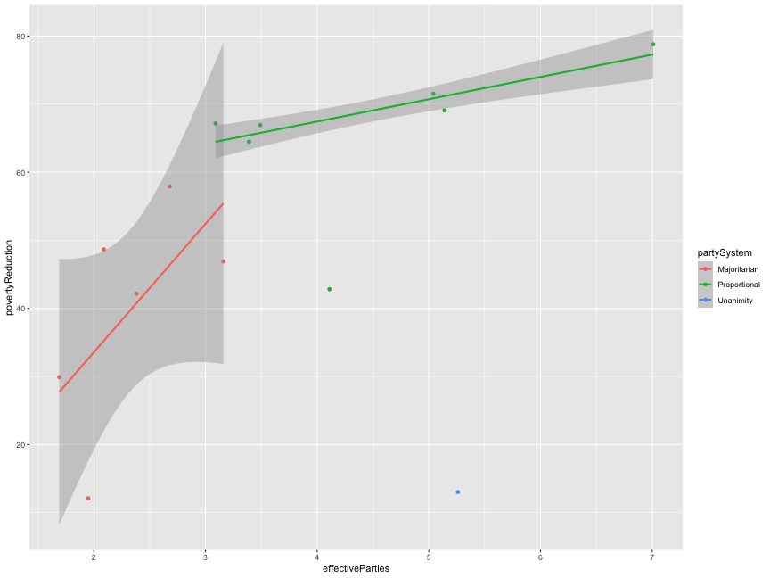<!-- --> ] --- count: false ## Why are there multiple smooth curves? -- inherit.aes .panel1-iver1-non_seq[ ```r ggplot(iver_data, aes(x = effectiveParties, y = povertyReduction, color = partySystem)) + geom_point( inherit.aes = TRUE, aes(x = effectiveParties, y = povertyReduction, color = partySystem) ) + geom_smooth( * inherit.aes = TRUE, * aes(x = effectiveParties, * y = povertyReduction, * color = partySystem), method = MASS::rlm ) ``` ] .panel2-iver1-non_seq[ <!-- --> ] <style> .panel1-iver1-non_seq { color: black; width: 38.6060606060606%; hight: 32%; float: left; padding-left: 1%; font-size: 80% } .panel2-iver1-non_seq { color: black; width: 59.3939393939394%; hight: 32%; float: left; padding-left: 1%; font-size: 80% } .panel3-iver1-non_seq { color: black; width: NA%; hight: 33%; float: left; padding-left: 1%; font-size: 80% } </style> --- count: false ## You can either overwrite the geom_smooth() layer .panel1-iver2-non_seq[ ```r ggplot(iver_data, aes(x = effectiveParties, y = povertyReduction, color = partySystem)) + geom_point( ) + geom_smooth( method = MASS::rlm ) ``` ] .panel2-iver2-non_seq[ <!-- --> ] --- count: false ## You can either overwrite the geom_smooth() layer .panel1-iver2-non_seq[ ```r ggplot(iver_data, aes(x = effectiveParties, y = povertyReduction, color = partySystem)) + geom_point( ) + geom_smooth( * aes(group = 1), method = MASS::rlm ) ``` ] .panel2-iver2-non_seq[ 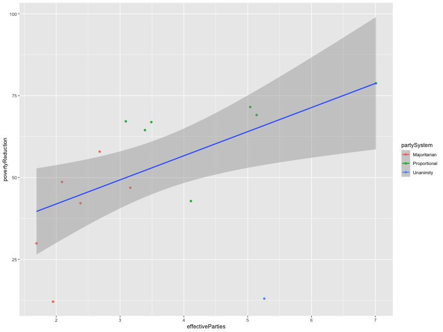<!-- --> ] <style> .panel1-iver2-non_seq { color: black; width: 38.6060606060606%; hight: 32%; float: left; padding-left: 1%; font-size: 80% } .panel2-iver2-non_seq { color: black; width: 59.3939393939394%; hight: 32%; float: left; padding-left: 1%; font-size: 80% } .panel3-iver2-non_seq { color: black; width: NA%; hight: 33%; float: left; padding-left: 1%; font-size: 80% } </style> --- count: false ## Or localize color aesthetics to the geom_point layer() .panel1-iver3-non_seq[ ```r ggplot(iver_data, aes(x = effectiveParties, y = povertyReduction)) + geom_point( ) + geom_smooth( method = MASS::rlm ) ``` ] .panel2-iver3-non_seq[ 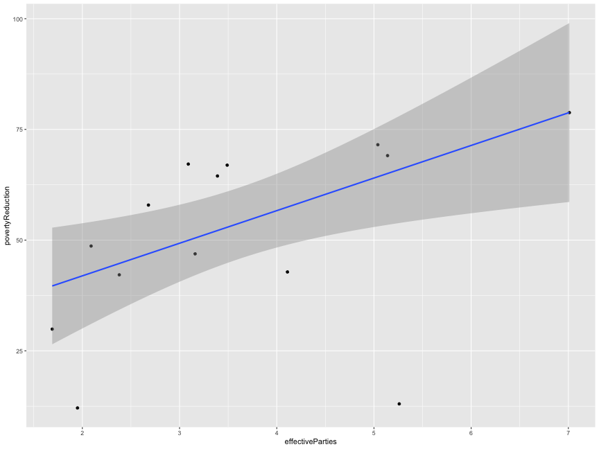<!-- --> ] --- count: false ## Or localize color aesthetics to the geom_point layer() .panel1-iver3-non_seq[ ```r ggplot(iver_data, aes(x = effectiveParties, y = povertyReduction)) + geom_point( * aes(color = partySystem) ) + geom_smooth( method = MASS::rlm ) ``` ] .panel2-iver3-non_seq[ 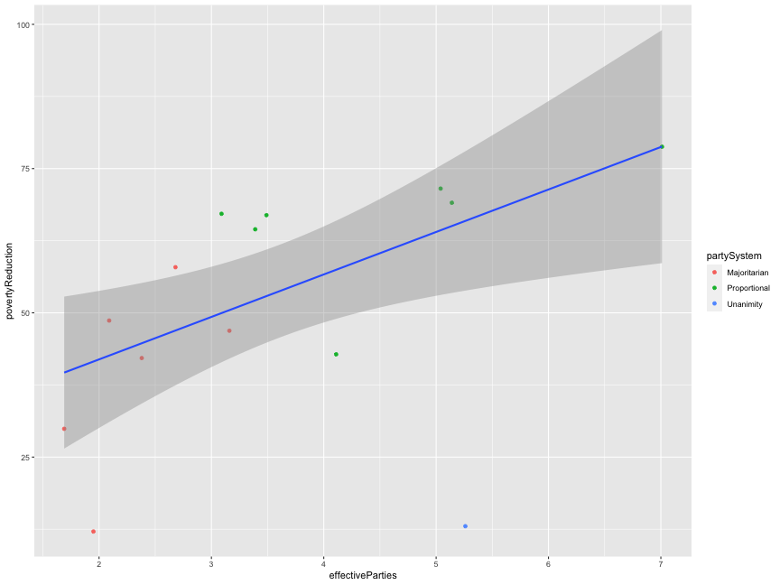<!-- --> ] <style> .panel1-iver3-non_seq { color: black; width: 38.6060606060606%; hight: 32%; float: left; padding-left: 1%; font-size: 80% } .panel2-iver3-non_seq { color: black; width: 59.3939393939394%; hight: 32%; float: left; padding-left: 1%; font-size: 80% } .panel3-iver3-non_seq { color: black; width: NA%; hight: 33%; float: left; padding-left: 1%; font-size: 80% } </style> --- ## A segue to a customized ggplot2 theme - Chris and I wrote a customized ggplot2 theme to implement a minimalist aesthetics -- - Can be downloaded here: https://students.washington.edu/kpleung/vis/theme_cavis.R -- - To use it ```r source("https://students.washington.edu/kpleung/vis/theme_cavis.R") # source(".../theme_cavis.R") if you have download and put it in your directory ``` -- - I'll use this theme throughout my vis; you don't have to (and suggestions are welcomed!) --- count: false ## Showcase customized theme .panel1-theme_cavis-rotate[ ```r ggplot(iris, aes(x = Sepal.Length, y = Petal.Length, color = Species)) + geom_point() + * theme_grey() ``` ] .panel2-theme_cavis-rotate[ 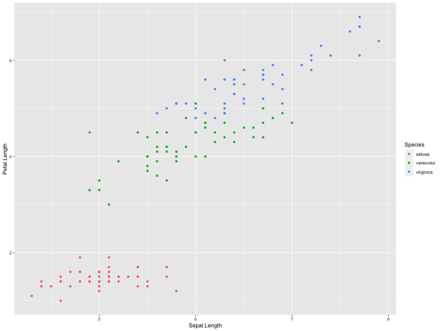<!-- --> ] --- count: false ## Showcase customized theme .panel1-theme_cavis-rotate[ ```r ggplot(iris, aes(x = Sepal.Length, y = Petal.Length, color = Species)) + geom_point() + * theme_cavis_hgrid ``` ] .panel2-theme_cavis-rotate[ 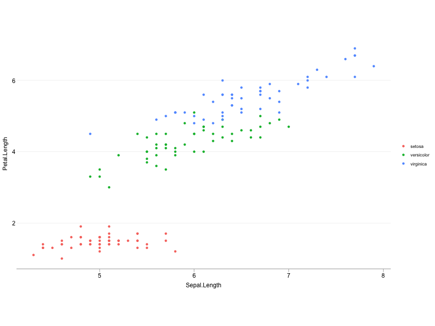<!-- --> ] --- count: false ## Showcase customized theme .panel1-theme_cavis-rotate[ ```r ggplot(iris, aes(x = Sepal.Length, y = Petal.Length, color = Species)) + geom_point() + * theme_cavis_vgrid ``` ] .panel2-theme_cavis-rotate[ <!-- --> ] --- count: false ## Showcase customized theme .panel1-theme_cavis-rotate[ ```r ggplot(iris, aes(x = Sepal.Length, y = Petal.Length, color = Species)) + geom_point() + * theme_cavis ``` ] .panel2-theme_cavis-rotate[ <!-- --> ] <style> .panel1-theme_cavis-rotate { color: black; width: 38.6060606060606%; hight: 32%; float: left; padding-left: 1%; font-size: 80% } .panel2-theme_cavis-rotate { color: black; width: 59.3939393939394%; hight: 32%; float: left; padding-left: 1%; font-size: 80% } .panel3-theme_cavis-rotate { color: black; width: NA%; hight: 33%; float: left; padding-left: 1%; font-size: 80% } </style> --- ## Visualization exercises: Electric vehicles in WA state - Data are taken from [Washington State Department of Licensing](https://data.wa.gov/Transportation/Electric-Vehicle-Population-Data/f6w7-q2d2) -- - "This dataset shows the Battery Electric Vehicles (BEVs) and Plug-in Hybrid Electric Vehicles (PHEVs) that are currently registered through Washington State Department of Licensing (DOL)." -- - Load the electric vehicles data ```r ev_data <- read_csv("data/ev_data.csv") head(ev_data) ``` ``` # A tibble: 6 × 8 county city make model model_year ev_type electric_range retail_price <chr> <chr> <chr> <chr> <dbl> <chr> <dbl> <dbl> 1 Kittitas Cle Elum TESLA MODE… 2020 Batter… 291 0 2 Chelan Chelan TESLA MODE… 2020 Batter… 322 0 3 Snohomish Snohomish TESLA MODE… 2018 Batter… 215 0 4 Thurston Tumwater FORD C-MAX 2014 Plug-i… 19 0 5 Kitsap Kingston FORD FUSI… 2013 Plug-i… 19 0 6 King Seattle NISS… LEAF 2018 Batter… 151 0 ``` --- ## Visualization exercises: Electric vehicles in WA state - Also some auxiliary county data with number of households and their median income ```r county_data <- read_csv("data/county_data.csv") head(county_data) ``` ``` # A tibble: 6 × 3 county hh_num hh_income <chr> <dbl> <dbl> 1 King 789232 68065 2 San Juan 7613 50726 3 Snohomish 268325 66300 4 Kitsap 97220 59549 5 Washington 2620076 57244 6 Thurston 100650 60930 ``` --- count: false ## EV in WA state: Which county has most EVs? .panel1-ev_by_county1-auto[ ```r # Count EVs by county *ev_data ``` ] .panel2-ev_by_county1-auto[ ``` # A tibble: 114,312 × 8 county city make model model_year ev_type electric_range retail_price <chr> <chr> <chr> <chr> <dbl> <chr> <dbl> <dbl> 1 Kittitas Cle Elum TESLA MODE… 2020 Batter… 291 0 2 Chelan Chelan TESLA MODE… 2020 Batter… 322 0 3 Snohomish Snohomi… TESLA MODE… 2018 Batter… 215 0 4 Thurston Tumwater FORD C-MAX 2014 Plug-i… 19 0 5 Kitsap Kingston FORD FUSI… 2013 Plug-i… 19 0 6 King Seattle NISS… LEAF 2018 Batter… 151 0 7 Skagit Mount V… AUDI E-TR… 2019 Batter… 204 0 8 Kitsap Port Or… NISS… LEAF 2019 Batter… 150 0 9 Snohomish Bothell TESLA MODE… 2020 Batter… 322 0 10 Yakima Tieton NISS… LEAF 2019 Batter… 150 0 # ℹ 114,302 more rows ``` ] --- count: false ## EV in WA state: Which county has most EVs? .panel1-ev_by_county1-auto[ ```r # Count EVs by county ev_data %>% * count(county) ``` ] .panel2-ev_by_county1-auto[ ``` # A tibble: 39 × 2 county n <chr> <int> 1 Adams 35 2 Asotin 46 3 Benton 1394 4 Chelan 654 5 Clallam 741 6 Clark 6827 7 Columbia 13 8 Cowlitz 576 9 Douglas 227 10 Ferry 27 # ℹ 29 more rows ``` ] --- count: false ## EV in WA state: Which county has most EVs? .panel1-ev_by_county1-auto[ ```r # Count EVs by county ev_data %>% count(county) %>% * mutate(county = fct_reorder(county, n)) ``` ] .panel2-ev_by_county1-auto[ ``` # A tibble: 39 × 2 county n <fct> <int> 1 Adams 35 2 Asotin 46 3 Benton 1394 4 Chelan 654 5 Clallam 741 6 Clark 6827 7 Columbia 13 8 Cowlitz 576 9 Douglas 227 10 Ferry 27 # ℹ 29 more rows ``` ] --- count: false ## EV in WA state: Which county has most EVs? .panel1-ev_by_county1-auto[ ```r # Count EVs by county ev_data %>% count(county) %>% mutate(county = fct_reorder(county, n)) %>% * arrange(desc(county)) ``` ] .panel2-ev_by_county1-auto[ ``` # A tibble: 39 × 2 county n <fct> <int> 1 King 60059 2 Snohomish 12720 3 Pierce 8684 4 Clark 6827 5 Thurston 4207 6 Kitsap 3902 7 Whatcom 2873 8 Spokane 2835 9 Benton 1394 10 Island 1307 # ℹ 29 more rows ``` ] --- count: false ## EV in WA state: Which county has most EVs? .panel1-ev_by_county1-auto[ ```r # Count EVs by county ev_data %>% count(county) %>% mutate(county = fct_reorder(county, n)) %>% arrange(desc(county)) -> * ev_by_county ``` ] .panel2-ev_by_county1-auto[ ] --- count: false ## EV in WA state: Which county has most EVs? .panel1-ev_by_county1-auto[ ```r # Count EVs by county ev_data %>% count(county) %>% mutate(county = fct_reorder(county, n)) %>% arrange(desc(county)) -> ev_by_county # Load scales package for labels and breaks *library(scales) ``` ] .panel2-ev_by_county1-auto[ ] <style> .panel1-ev_by_county1-auto { color: black; width: 88.2%; hight: 32%; float: top; padding-left: 1%; font-size: 80% } .panel2-ev_by_county1-auto { color: black; width: 9.8%; hight: 32%; float: top; padding-left: 1%; font-size: 80% } .panel3-ev_by_county1-auto { color: black; width: NA%; hight: 33%; float: top; padding-left: 1%; font-size: 80% } </style> --- count: false ## EV in WA state: Which county has most EVs? .panel1-ev_by_county2-non_seq[ ```r ggplot(ev_by_county, aes(y = county, x = n)) + theme_cavis_vgrid + geom_point() ``` ] .panel2-ev_by_county2-non_seq[ 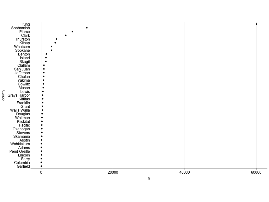<!-- --> ] --- count: false ## EV in WA state: Which county has most EVs? .panel1-ev_by_county2-non_seq[ ```r ggplot(ev_by_county, aes(y = county, x = n)) + theme_cavis_vgrid + geom_point() + * geom_col( * ) ``` ] .panel2-ev_by_county2-non_seq[ 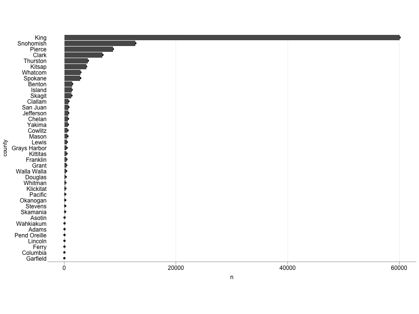<!-- --> ] --- count: false ## EV in WA state: Which county has most EVs? .panel1-ev_by_county2-non_seq[ ```r ggplot(ev_by_county, aes(y = county, x = n)) + theme_cavis_vgrid + geom_point() + geom_col( * width = 0.05, * alpha = 0.5 ) ``` ] .panel2-ev_by_county2-non_seq[ 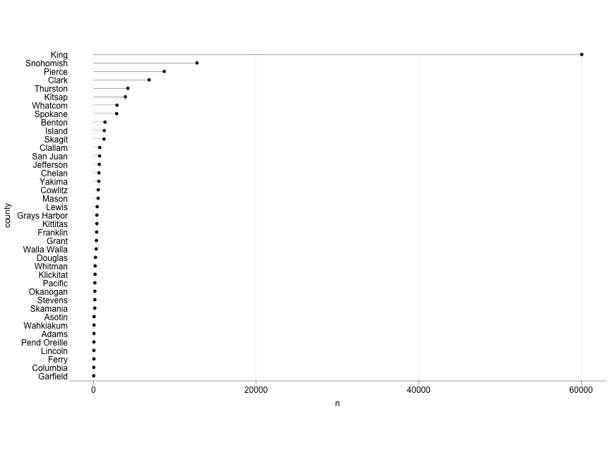<!-- --> ] --- count: false ## EV in WA state: Which county has most EVs? .panel1-ev_by_county2-non_seq[ ```r ggplot(ev_by_county, aes(y = county, x = n)) + theme_cavis_vgrid + geom_point() + geom_col( width = 0.05, alpha = 0.5 ) + * scale_x_continuous( * trans = "log10", * ) ``` ] .panel2-ev_by_county2-non_seq[ 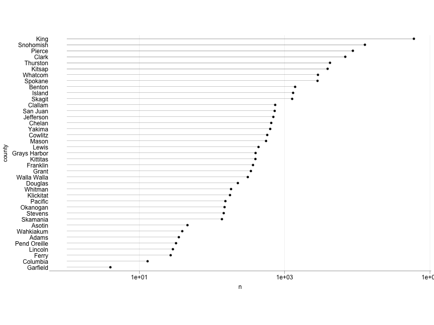<!-- --> ] --- count: false ## EV in WA state: Which county has most EVs? .panel1-ev_by_county2-non_seq[ ```r ggplot(ev_by_county, aes(y = county, x = n)) + theme_cavis_vgrid + geom_point() + geom_col( width = 0.05, alpha = 0.5 ) + scale_x_continuous( trans = "log10", * breaks = 10^(0:5), * labels = scales::label_comma(), ) ``` ] .panel2-ev_by_county2-non_seq[ 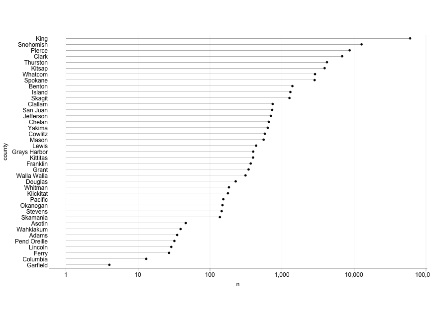<!-- --> ] --- count: false ## EV in WA state: Which county has most EVs? .panel1-ev_by_county2-non_seq[ ```r ggplot(ev_by_county, aes(y = county, x = n)) + theme_cavis_vgrid + geom_point() + geom_col( width = 0.05, alpha = 0.5 ) + scale_x_continuous( trans = "log10", breaks = 10^(0:5), labels = scales::label_comma(), ) + * geom_text( * aes(label = n), * ) ``` ] .panel2-ev_by_county2-non_seq[ 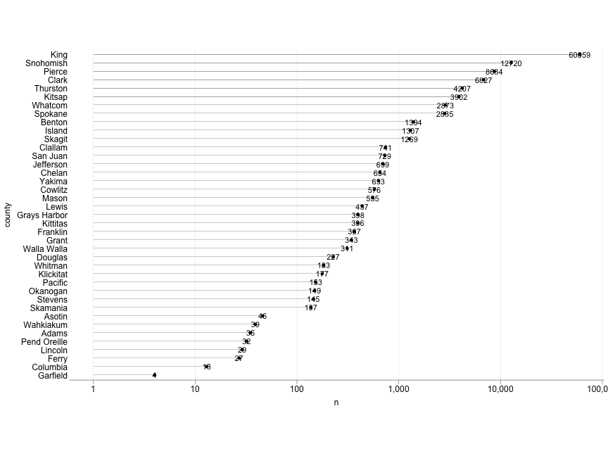<!-- --> ] --- count: false ## EV in WA state: Which county has most EVs? .panel1-ev_by_county2-non_seq[ ```r ggplot(ev_by_county, aes(y = county, x = n)) + theme_cavis_vgrid + geom_point() + geom_col( width = 0.05, alpha = 0.5 ) + scale_x_continuous( trans = "log10", breaks = 10^(0:5), labels = scales::label_comma(), ) + geom_text( aes(label = n), * nudge_x = 0.15 ) ``` ] .panel2-ev_by_county2-non_seq[ 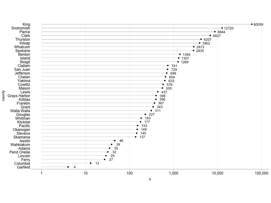<!-- --> ] --- count: false ## EV in WA state: Which county has most EVs? .panel1-ev_by_county2-non_seq[ ```r ggplot(ev_by_county, aes(y = county, x = n)) + theme_cavis_vgrid + geom_point() + geom_col( width = 0.05, alpha = 0.5 ) + scale_x_continuous( trans = "log10", breaks = 10^(0:5), labels = scales::label_comma(), ) + geom_text( * data = slice_max(ev_by_county, n, n = 10), aes(label = n), nudge_x = 0.15 ) ``` ] .panel2-ev_by_county2-non_seq[ 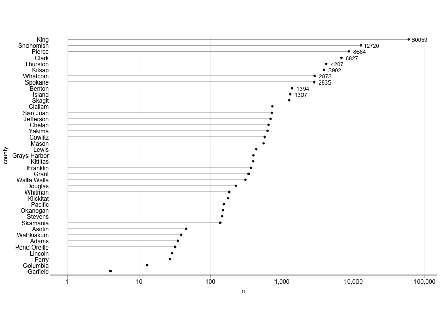<!-- --> ] --- count: false ## EV in WA state: Which county has most EVs? .panel1-ev_by_county2-non_seq[ ```r ggplot(ev_by_county, aes(y = county, x = n)) + theme_cavis_vgrid + geom_point() + geom_col( width = 0.05, alpha = 0.5 ) + scale_x_continuous( trans = "log10", breaks = 10^(0:5), labels = scales::label_comma(), ) + geom_text( data = slice_max(ev_by_county, n, n = 10), aes(label = n), nudge_x = 0.15 ) + * labs(y = NULL, x = "Total number of EVs") ``` ] .panel2-ev_by_county2-non_seq[ 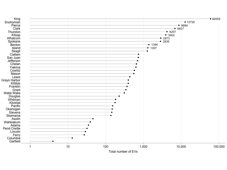<!-- --> ] <style> .panel1-ev_by_county2-non_seq { color: black; width: 49%; hight: 32%; float: left; padding-left: 1%; font-size: 80% } .panel2-ev_by_county2-non_seq { color: black; width: 49%; hight: 32%; float: left; padding-left: 1%; font-size: 80% } .panel3-ev_by_county2-non_seq { color: black; width: NA%; hight: 33%; float: left; padding-left: 1%; font-size: 80% } </style> --- count: false ## EV in WA state: Trend of number of EVs across county .panel1-ev_by_countyYear1-auto[ ```r # Count number of EVs by county *ev_data ``` ] .panel2-ev_by_countyYear1-auto[ ``` # A tibble: 114,312 × 8 county city make model model_year ev_type electric_range retail_price <chr> <chr> <chr> <chr> <dbl> <chr> <dbl> <dbl> 1 Kittitas Cle Elum TESLA MODE… 2020 Batter… 291 0 2 Chelan Chelan TESLA MODE… 2020 Batter… 322 0 3 Snohomish Snohomi… TESLA MODE… 2018 Batter… 215 0 4 Thurston Tumwater FORD C-MAX 2014 Plug-i… 19 0 5 Kitsap Kingston FORD FUSI… 2013 Plug-i… 19 0 6 King Seattle NISS… LEAF 2018 Batter… 151 0 7 Skagit Mount V… AUDI E-TR… 2019 Batter… 204 0 8 Kitsap Port Or… NISS… LEAF 2019 Batter… 150 0 9 Snohomish Bothell TESLA MODE… 2020 Batter… 322 0 10 Yakima Tieton NISS… LEAF 2019 Batter… 150 0 # ℹ 114,302 more rows ``` ] --- count: false ## EV in WA state: Trend of number of EVs across county .panel1-ev_by_countyYear1-auto[ ```r # Count number of EVs by county ev_data %>% * group_by(model_year, county) ``` ] .panel2-ev_by_countyYear1-auto[ ``` # A tibble: 114,312 × 8 # Groups: model_year, county [497] county city make model model_year ev_type electric_range retail_price <chr> <chr> <chr> <chr> <dbl> <chr> <dbl> <dbl> 1 Kittitas Cle Elum TESLA MODE… 2020 Batter… 291 0 2 Chelan Chelan TESLA MODE… 2020 Batter… 322 0 3 Snohomish Snohomi… TESLA MODE… 2018 Batter… 215 0 4 Thurston Tumwater FORD C-MAX 2014 Plug-i… 19 0 5 Kitsap Kingston FORD FUSI… 2013 Plug-i… 19 0 6 King Seattle NISS… LEAF 2018 Batter… 151 0 7 Skagit Mount V… AUDI E-TR… 2019 Batter… 204 0 8 Kitsap Port Or… NISS… LEAF 2019 Batter… 150 0 9 Snohomish Bothell TESLA MODE… 2020 Batter… 322 0 10 Yakima Tieton NISS… LEAF 2019 Batter… 150 0 # ℹ 114,302 more rows ``` ] --- count: false ## EV in WA state: Trend of number of EVs across county .panel1-ev_by_countyYear1-auto[ ```r # Count number of EVs by county ev_data %>% group_by(model_year, county) %>% * count() ``` ] .panel2-ev_by_countyYear1-auto[ ``` # A tibble: 497 × 3 # Groups: model_year, county [497] model_year county n <dbl> <chr> <int> 1 1997 Snohomish 1 2 1998 Clallam 1 3 1999 Pierce 1 4 1999 Skagit 1 5 1999 Whatcom 1 6 2000 King 4 7 2000 San Juan 2 8 2000 Snohomish 1 9 2000 Whatcom 2 10 2002 Clallam 1 # ℹ 487 more rows ``` ] --- count: false ## EV in WA state: Trend of number of EVs across county .panel1-ev_by_countyYear1-auto[ ```r # Count number of EVs by county ev_data %>% group_by(model_year, county) %>% count() -> * ev_by_countyYear ``` ] .panel2-ev_by_countyYear1-auto[ ] <style> .panel1-ev_by_countyYear1-auto { color: black; width: 88.2%; hight: 32%; float: top; padding-left: 1%; font-size: 80% } .panel2-ev_by_countyYear1-auto { color: black; width: 9.8%; hight: 32%; float: top; padding-left: 1%; font-size: 80% } .panel3-ev_by_countyYear1-auto { color: black; width: NA%; hight: 33%; float: top; padding-left: 1%; font-size: 80% } </style> --- count: false ## EV in WA state: Trend of number of EVs across county .panel1-ev_by_countyYear2-auto[ ```r *ggplot(ev_by_countyYear, * aes(x = model_year, * y = n, * group = county, * color = county == "King")) ``` ] .panel2-ev_by_countyYear2-auto[ <!-- --> ] --- count: false ## EV in WA state: Trend of number of EVs across county .panel1-ev_by_countyYear2-auto[ ```r ggplot(ev_by_countyYear, aes(x = model_year, y = n, group = county, color = county == "King")) + * theme_cavis_hgrid ``` ] .panel2-ev_by_countyYear2-auto[ <!-- --> ] --- count: false ## EV in WA state: Trend of number of EVs across county .panel1-ev_by_countyYear2-auto[ ```r ggplot(ev_by_countyYear, aes(x = model_year, y = n, group = county, color = county == "King")) + theme_cavis_hgrid + * geom_line() ``` ] .panel2-ev_by_countyYear2-auto[ <!-- --> ] --- count: false ## EV in WA state: Trend of number of EVs across county .panel1-ev_by_countyYear2-auto[ ```r ggplot(ev_by_countyYear, aes(x = model_year, y = n, group = county, color = county == "King")) + theme_cavis_hgrid + geom_line() + * scale_y_continuous(trans = "log10") ``` ] .panel2-ev_by_countyYear2-auto[ <!-- --> ] --- count: false ## EV in WA state: Trend of number of EVs across county .panel1-ev_by_countyYear2-auto[ ```r ggplot(ev_by_countyYear, aes(x = model_year, y = n, group = county, color = county == "King")) + theme_cavis_hgrid + geom_line() + scale_y_continuous(trans = "log10") + * scale_color_manual(values = c("grey90", "red")) ``` ] .panel2-ev_by_countyYear2-auto[ <!-- --> ] --- count: false ## EV in WA state: Trend of number of EVs across county .panel1-ev_by_countyYear2-auto[ ```r ggplot(ev_by_countyYear, aes(x = model_year, y = n, group = county, color = county == "King")) + theme_cavis_hgrid + geom_line() + scale_y_continuous(trans = "log10") + scale_color_manual(values = c("grey90", "red")) + * guides(color = "none") ``` ] .panel2-ev_by_countyYear2-auto[ 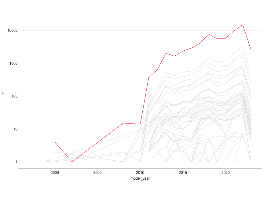<!-- --> ] --- count: false ## EV in WA state: Trend of number of EVs across county .panel1-ev_by_countyYear2-auto[ ```r ggplot(ev_by_countyYear, aes(x = model_year, y = n, group = county, color = county == "King")) + theme_cavis_hgrid + geom_line() + scale_y_continuous(trans = "log10") + scale_color_manual(values = c("grey90", "red")) + guides(color = "none") + * annotate("text", x = 2018, y = 13000, * label = "King County", * color = "red") ``` ] .panel2-ev_by_countyYear2-auto[ 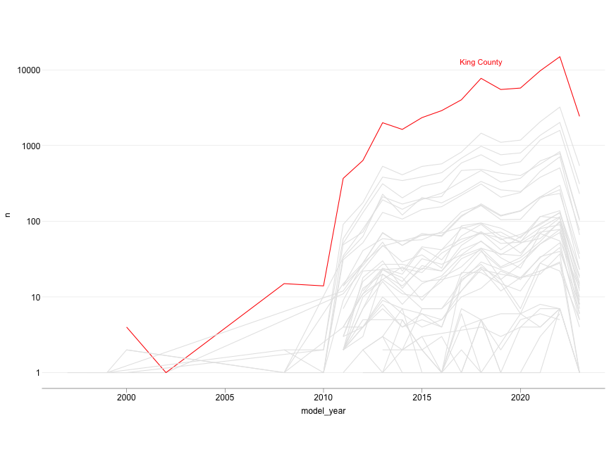<!-- --> ] --- count: false ## EV in WA state: Trend of number of EVs across county .panel1-ev_by_countyYear2-auto[ ```r ggplot(ev_by_countyYear, aes(x = model_year, y = n, group = county, color = county == "King")) + theme_cavis_hgrid + geom_line() + scale_y_continuous(trans = "log10") + scale_color_manual(values = c("grey90", "red")) + guides(color = "none") + annotate("text", x = 2018, y = 13000, label = "King County", color = "red") + * geom_vline(xintercept = 2012, linetype = 2, * color = "grey45") ``` ] .panel2-ev_by_countyYear2-auto[ 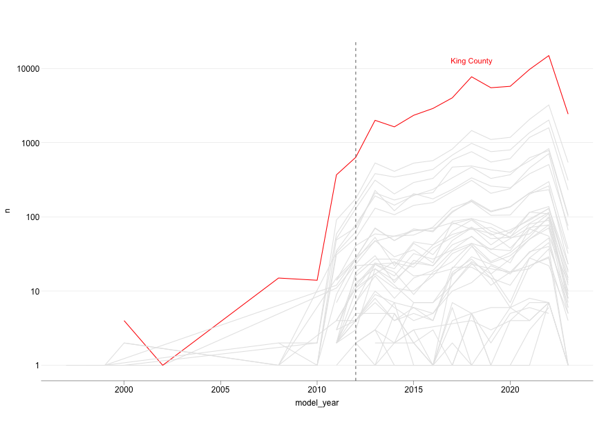<!-- --> ] --- count: false ## EV in WA state: Trend of number of EVs across county .panel1-ev_by_countyYear2-auto[ ```r ggplot(ev_by_countyYear, aes(x = model_year, y = n, group = county, color = county == "King")) + theme_cavis_hgrid + geom_line() + scale_y_continuous(trans = "log10") + scale_color_manual(values = c("grey90", "red")) + guides(color = "none") + annotate("text", x = 2018, y = 13000, label = "King County", color = "red") + geom_vline(xintercept = 2012, linetype = 2, color = "grey45") + * annotate("text", x = 2010, y = 15000, * label = "Tesla Model S\nintroduced", * color = "black") ``` ] .panel2-ev_by_countyYear2-auto[ 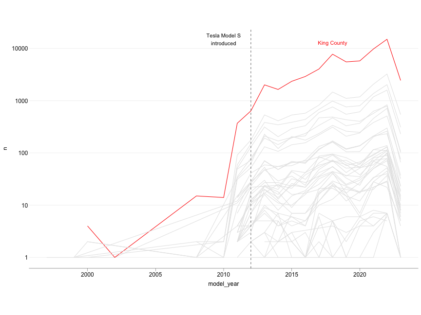<!-- --> ] --- count: false ## EV in WA state: Trend of number of EVs across county .panel1-ev_by_countyYear2-auto[ ```r ggplot(ev_by_countyYear, aes(x = model_year, y = n, group = county, color = county == "King")) + theme_cavis_hgrid + geom_line() + scale_y_continuous(trans = "log10") + scale_color_manual(values = c("grey90", "red")) + guides(color = "none") + annotate("text", x = 2018, y = 13000, label = "King County", color = "red") + geom_vline(xintercept = 2012, linetype = 2, color = "grey45") + annotate("text", x = 2010, y = 15000, label = "Tesla Model S\nintroduced", color = "black") + * labs(y = "Number of registed EVs", x = NULL) ``` ] .panel2-ev_by_countyYear2-auto[ 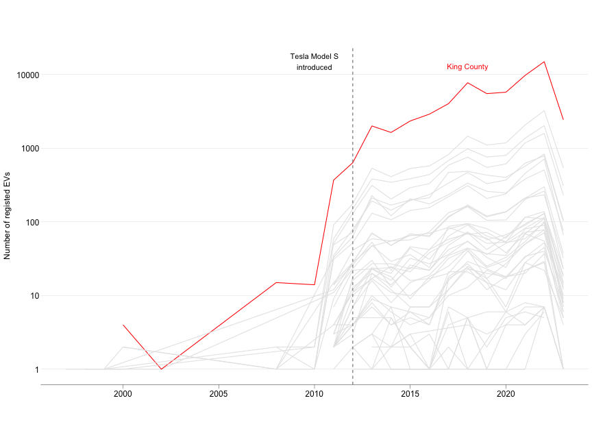<!-- --> ] <style> .panel1-ev_by_countyYear2-auto { color: black; width: 49%; hight: 32%; float: left; padding-left: 1%; font-size: 80% } .panel2-ev_by_countyYear2-auto { color: black; width: 49%; hight: 32%; float: left; padding-left: 1%; font-size: 80% } .panel3-ev_by_countyYear2-auto { color: black; width: NA%; hight: 33%; float: left; padding-left: 1%; font-size: 80% } </style> --- count: false ## EV in WA state: Relationship between price and range .panel1-price_range1-auto[ ```r *ev_data ``` ] .panel2-price_range1-auto[ ``` # A tibble: 114,312 × 8 county city make model model_year ev_type electric_range retail_price <chr> <chr> <chr> <chr> <dbl> <chr> <dbl> <dbl> 1 Kittitas Cle Elum TESLA MODE… 2020 Batter… 291 0 2 Chelan Chelan TESLA MODE… 2020 Batter… 322 0 3 Snohomish Snohomi… TESLA MODE… 2018 Batter… 215 0 4 Thurston Tumwater FORD C-MAX 2014 Plug-i… 19 0 5 Kitsap Kingston FORD FUSI… 2013 Plug-i… 19 0 6 King Seattle NISS… LEAF 2018 Batter… 151 0 7 Skagit Mount V… AUDI E-TR… 2019 Batter… 204 0 8 Kitsap Port Or… NISS… LEAF 2019 Batter… 150 0 9 Snohomish Bothell TESLA MODE… 2020 Batter… 322 0 10 Yakima Tieton NISS… LEAF 2019 Batter… 150 0 # ℹ 114,302 more rows ``` ] --- count: false ## EV in WA state: Relationship between price and range .panel1-price_range1-auto[ ```r ev_data %>% * distinct(make, model, model_year, ev_type, electric_range, retail_price) ``` ] .panel2-price_range1-auto[ ``` # A tibble: 427 × 6 make model model_year ev_type electric_range retail_price <chr> <chr> <dbl> <chr> <dbl> <dbl> 1 TESLA MODEL Y 2020 Battery Electric Vehic… 291 0 2 TESLA MODEL 3 2020 Battery Electric Vehic… 322 0 3 TESLA MODEL 3 2018 Battery Electric Vehic… 215 0 4 FORD C-MAX 2014 Plug-in Hybrid Electri… 19 0 5 FORD FUSION 2013 Plug-in Hybrid Electri… 19 0 6 NISSAN LEAF 2018 Battery Electric Vehic… 151 0 7 AUDI E-TRON 2019 Battery Electric Vehic… 204 0 8 NISSAN LEAF 2019 Battery Electric Vehic… 150 0 9 KIA NIRO 2018 Plug-in Hybrid Electri… 26 0 10 NISSAN LEAF 2012 Battery Electric Vehic… 73 0 # ℹ 417 more rows ``` ] --- count: false ## EV in WA state: Relationship between price and range .panel1-price_range1-auto[ ```r ev_data %>% distinct(make, model, model_year, ev_type, electric_range, retail_price) %>% * filter(retail_price > 0 & electric_range > 0) ``` ] .panel2-price_range1-auto[ ``` # A tibble: 32 × 6 make model model_year ev_type electric_range retail_price <chr> <chr> <dbl> <chr> <dbl> <dbl> 1 KIA SOUL 2016 Battery Electric … 93 31950 2 KIA SOUL EV 2018 Battery Electric … 111 33950 3 TESLA MODEL S 2013 Battery Electric … 208 69900 4 TESLA MODEL S 2014 Battery Electric … 208 69900 5 CHRYSLER PACIFICA 2019 Plug-in Hybrid El… 32 39995 6 MINI COUNTRYMAN 2018 Plug-in Hybrid El… 12 36800 7 BMW 530E 2018 Plug-in Hybrid El… 14 54950 8 TESLA ROADSTER 2010 Battery Electric … 245 110950 9 KIA SOUL EV 2017 Battery Electric … 93 32250 10 VOLVO XC60 2018 Plug-in Hybrid El… 17 52900 # ℹ 22 more rows ``` ] --- count: false ## EV in WA state: Relationship between price and range .panel1-price_range1-auto[ ```r ev_data %>% distinct(make, model, model_year, ev_type, electric_range, retail_price) %>% filter(retail_price > 0 & electric_range > 0) -> * ev_models ``` ] .panel2-price_range1-auto[ ] --- count: false ## EV in WA state: Relationship between price and range .panel1-price_range1-auto[ ```r ev_data %>% distinct(make, model, model_year, ev_type, electric_range, retail_price) %>% filter(retail_price > 0 & electric_range > 0) -> ev_models # load packages *library(ggrepel) ``` ] .panel2-price_range1-auto[ ] --- count: false ## EV in WA state: Relationship between price and range .panel1-price_range1-auto[ ```r ev_data %>% distinct(make, model, model_year, ev_type, electric_range, retail_price) %>% filter(retail_price > 0 & electric_range > 0) -> ev_models # load packages library(ggrepel) *library(RColorBrewer) ``` ] .panel2-price_range1-auto[ ] <style> .panel1-price_range1-auto { color: black; width: 88.2%; hight: 32%; float: top; padding-left: 1%; font-size: 80% } .panel2-price_range1-auto { color: black; width: 9.8%; hight: 32%; float: top; padding-left: 1%; font-size: 80% } .panel3-price_range1-auto { color: black; width: NA%; hight: 33%; float: top; padding-left: 1%; font-size: 80% } </style> --- ## A segue to choosing colors - Use `RColorBrewer` package to choose colors -- - Choose between sequential, diverging or qualitative palettes based on your data -- - Check out this [website](https://colorbrewer2.org/) --- count: false ## A segue to choosing colors .panel1-color1-auto[ ```r *RColorBrewer::display.brewer.all() ``` ] .panel2-color1-auto[ <!-- --> ] --- count: false ## A segue to choosing colors .panel1-color1-auto[ ```r RColorBrewer::display.brewer.all() *colors <- brewer.pal(n = 5, name = "Set1") ``` ] .panel2-color1-auto[ 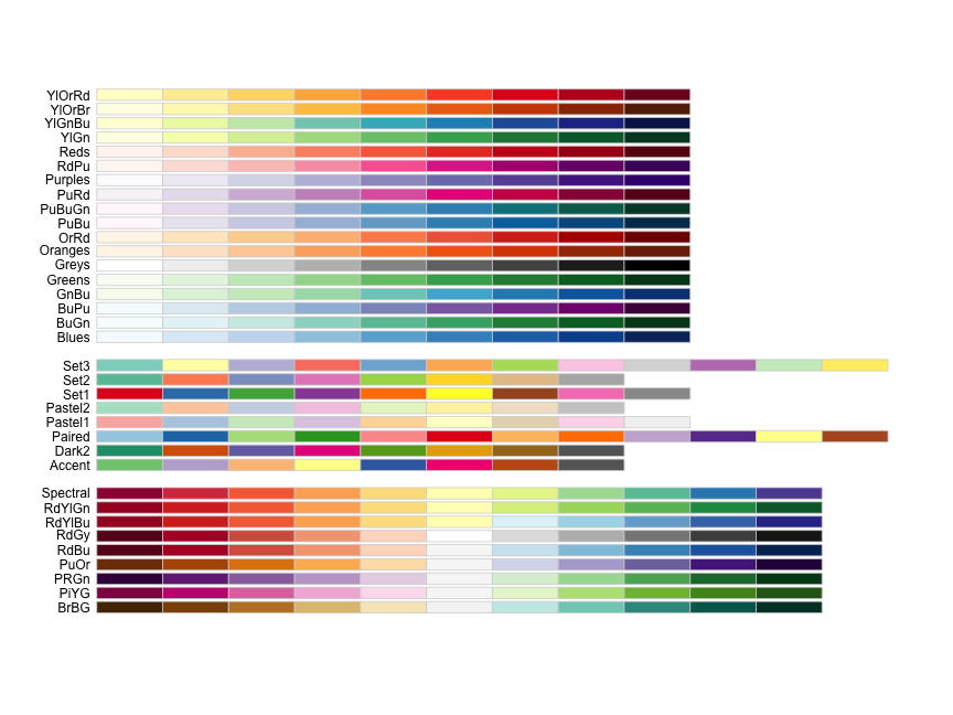<!-- --> ] --- count: false ## A segue to choosing colors .panel1-color1-auto[ ```r RColorBrewer::display.brewer.all() colors <- brewer.pal(n = 5, name = "Set1") *print(colors) ``` ] .panel2-color1-auto[ <!-- --> ``` [1] "#E41A1C" "#377EB8" "#4DAF4A" "#984EA3" "#FF7F00" ``` ] --- count: false ## A segue to choosing colors .panel1-color1-auto[ ```r RColorBrewer::display.brewer.all() colors <- brewer.pal(n = 5, name = "Set1") print(colors) *blue <- colors[2] ``` ] .panel2-color1-auto[ <!-- --> ``` [1] "#E41A1C" "#377EB8" "#4DAF4A" "#984EA3" "#FF7F00" ``` ] --- count: false ## A segue to choosing colors .panel1-color1-auto[ ```r RColorBrewer::display.brewer.all() colors <- brewer.pal(n = 5, name = "Set1") print(colors) blue <- colors[2] *orange <- colors[5] ``` ] .panel2-color1-auto[ <!-- --> ``` [1] "#E41A1C" "#377EB8" "#4DAF4A" "#984EA3" "#FF7F00" ``` ] <style> .panel1-color1-auto { color: black; width: 49%; hight: 32%; float: left; padding-left: 1%; font-size: 80% } .panel2-color1-auto { color: black; width: 49%; hight: 32%; float: left; padding-left: 1%; font-size: 80% } .panel3-color1-auto { color: black; width: NA%; hight: 33%; float: left; padding-left: 1%; font-size: 80% } </style> --- count: false ## EV in WA state: Relationship between price and range .panel1-price_range2-non_seq[ ```r ggplot(ev_models, aes(x = electric_range, y = retail_price, color = ev_type, fill = ev_type)) + theme_cavis_hgrid + geom_point(alpha = 0.75) ``` ] .panel2-price_range2-non_seq[ 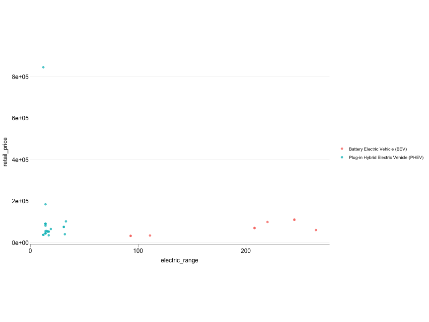<!-- --> ] --- count: false ## EV in WA state: Relationship between price and range .panel1-price_range2-non_seq[ ```r ggplot(ev_models, aes(x = electric_range, y = retail_price, color = ev_type, fill = ev_type)) + theme_cavis_hgrid + geom_point(alpha = 0.75) + * geom_smooth(method = "lm", * alpha = 0.15, size = 0.45) ``` ] .panel2-price_range2-non_seq[ 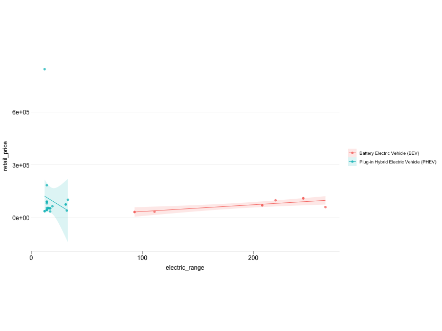<!-- --> ] --- count: false ## EV in WA state: Relationship between price and range .panel1-price_range2-non_seq[ ```r ggplot(ev_models, aes(x = electric_range, y = retail_price, color = ev_type, fill = ev_type)) + theme_cavis_hgrid + geom_point(alpha = 0.75) + geom_smooth(method = "lm", alpha = 0.15, size = 0.45) + * scale_x_continuous(trans = "log2") ``` ] .panel2-price_range2-non_seq[ 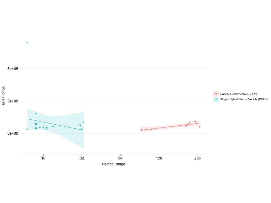<!-- --> ] --- count: false ## EV in WA state: Relationship between price and range .panel1-price_range2-non_seq[ ```r ggplot(ev_models, aes(x = electric_range, y = retail_price, color = ev_type, fill = ev_type)) + theme_cavis_hgrid + geom_point(alpha = 0.75) + geom_smooth(method = "lm", alpha = 0.15, size = 0.45) + scale_x_continuous(trans = "log2") + * scale_y_continuous(trans = "log10", * labels = label_dollar()) ``` ] .panel2-price_range2-non_seq[ 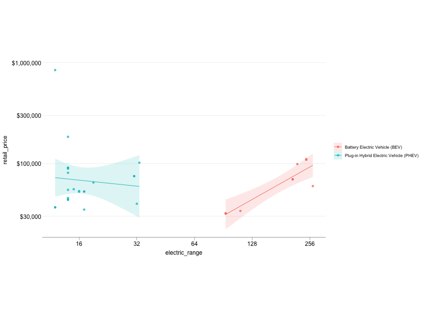<!-- --> ] --- count: false ## EV in WA state: Relationship between price and range .panel1-price_range2-non_seq[ ```r ggplot(ev_models, aes(x = electric_range, y = retail_price, color = ev_type, fill = ev_type)) + theme_cavis_hgrid + geom_point(alpha = 0.75) + geom_smooth(method = "lm", alpha = 0.15, size = 0.45) + scale_x_continuous(trans = "log2") + scale_y_continuous(trans = "log10", labels = label_dollar())+ * scale_color_manual(values = c(blue, orange)) + * scale_fill_manual(values = c(blue, orange)) ``` ] .panel2-price_range2-non_seq[ 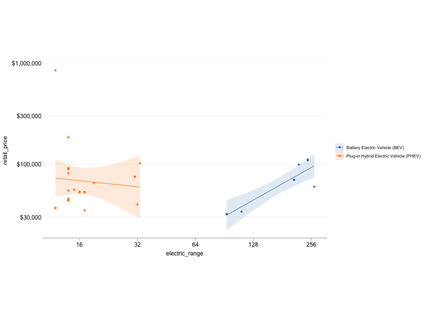<!-- --> ] --- count: false ## EV in WA state: Relationship between price and range .panel1-price_range2-non_seq[ ```r ggplot(ev_models, aes(x = electric_range, y = retail_price, color = ev_type, fill = ev_type)) + theme_cavis_hgrid + geom_point(alpha = 0.75) + geom_smooth(method = "lm", alpha = 0.15, size = 0.45) + scale_x_continuous(trans = "log2") + scale_y_continuous(trans = "log10", labels = label_dollar())+ scale_color_manual(values = c(blue, orange)) + scale_fill_manual(values = c(blue, orange)) + * geom_text_repel( * aes(label = paste(make, model, model_year)), * ) ``` ] .panel2-price_range2-non_seq[ 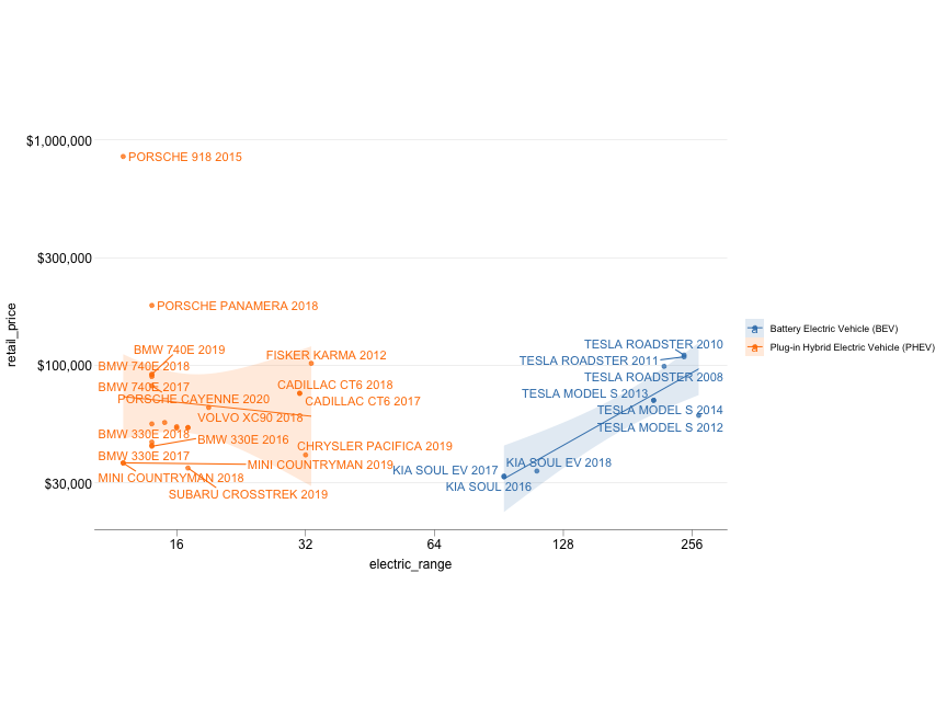<!-- --> ] --- count: false ## EV in WA state: Relationship between price and range .panel1-price_range2-non_seq[ ```r ggplot(ev_models, aes(x = electric_range, y = retail_price, color = ev_type, fill = ev_type)) + theme_cavis_hgrid + geom_point(alpha = 0.75) + geom_smooth(method = "lm", alpha = 0.15, size = 0.45) + scale_x_continuous(trans = "log2") + scale_y_continuous(trans = "log10", labels = label_dollar())+ scale_color_manual(values = c(blue, orange)) + scale_fill_manual(values = c(blue, orange)) + geom_text_repel( aes(label = paste(make, model, model_year)), * show.legend = FALSE, * size = 3, alpha = 0.75 ) ``` ] .panel2-price_range2-non_seq[ <!-- --> ] --- count: false ## EV in WA state: Relationship between price and range .panel1-price_range2-non_seq[ ```r ggplot(ev_models, aes(x = electric_range, y = retail_price, color = ev_type, fill = ev_type)) + theme_cavis_hgrid + geom_point(alpha = 0.75) + geom_smooth(method = "lm", alpha = 0.15, size = 0.45) + scale_x_continuous(trans = "log2") + scale_y_continuous(trans = "log10", labels = label_dollar())+ scale_color_manual(values = c(blue, orange)) + scale_fill_manual(values = c(blue, orange)) + geom_text_repel( aes(label = paste(make, model, model_year)), show.legend = FALSE, size = 3, alpha = 0.75 ) + * theme(legend.position = "top") ``` ] .panel2-price_range2-non_seq[ <!-- --> ] --- count: false ## EV in WA state: Relationship between price and range .panel1-price_range2-non_seq[ ```r ggplot(ev_models, aes(x = electric_range, y = retail_price, color = ev_type, fill = ev_type)) + theme_cavis_hgrid + geom_point(alpha = 0.75) + geom_smooth(method = "lm", alpha = 0.15, size = 0.45) + scale_x_continuous(trans = "log2") + scale_y_continuous(trans = "log10", labels = label_dollar())+ scale_color_manual(values = c(blue, orange)) + scale_fill_manual(values = c(blue, orange)) + geom_text_repel( aes(label = paste(make, model, model_year)), show.legend = FALSE, size = 3, alpha = 0.75 ) + theme(legend.position = "top") + * labs(y = "Retail price", x = "Electric range (mile)") ``` ] .panel2-price_range2-non_seq[ <!-- --> ] <style> .panel1-price_range2-non_seq { color: black; width: 49%; hight: 32%; float: left; padding-left: 1%; font-size: 80% } .panel2-price_range2-non_seq { color: black; width: 49%; hight: 32%; float: left; padding-left: 1%; font-size: 80% } .panel3-price_range2-non_seq { color: black; width: NA%; hight: 33%; float: left; padding-left: 1%; font-size: 80% } </style> --- ## Another segue: how to properly save a graph? - Don't use the `Export` interface in your RStudio -- - Use code for reproducibility; explicitly declare parameters (e.g. for width, height and aspect ratio) -- - Use `ggsave()` function for ggplot2 objects ```r width <- 12 ggsave("ev_bivariate.pdf", width = width, height = width/1.618) ``` --- count: false ## EV in WA state: Shares of makes across counties .panel1-make_share_fail-auto[ ```r # bad example *ev_data ``` ] .panel2-make_share_fail-auto[ ``` # A tibble: 114,312 × 8 county city make model model_year ev_type electric_range retail_price <chr> <chr> <chr> <chr> <dbl> <chr> <dbl> <dbl> 1 Kittitas Cle Elum TESLA MODE… 2020 Batter… 291 0 2 Chelan Chelan TESLA MODE… 2020 Batter… 322 0 3 Snohomish Snohomi… TESLA MODE… 2018 Batter… 215 0 4 Thurston Tumwater FORD C-MAX 2014 Plug-i… 19 0 5 Kitsap Kingston FORD FUSI… 2013 Plug-i… 19 0 6 King Seattle NISS… LEAF 2018 Batter… 151 0 7 Skagit Mount V… AUDI E-TR… 2019 Batter… 204 0 8 Kitsap Port Or… NISS… LEAF 2019 Batter… 150 0 9 Snohomish Bothell TESLA MODE… 2020 Batter… 322 0 10 Yakima Tieton NISS… LEAF 2019 Batter… 150 0 # ℹ 114,302 more rows ``` ] --- count: false ## EV in WA state: Shares of makes across counties .panel1-make_share_fail-auto[ ```r # bad example ev_data %>% * group_by(county, make) ``` ] .panel2-make_share_fail-auto[ ``` # A tibble: 114,312 × 8 # Groups: county, make [829] county city make model model_year ev_type electric_range retail_price <chr> <chr> <chr> <chr> <dbl> <chr> <dbl> <dbl> 1 Kittitas Cle Elum TESLA MODE… 2020 Batter… 291 0 2 Chelan Chelan TESLA MODE… 2020 Batter… 322 0 3 Snohomish Snohomi… TESLA MODE… 2018 Batter… 215 0 4 Thurston Tumwater FORD C-MAX 2014 Plug-i… 19 0 5 Kitsap Kingston FORD FUSI… 2013 Plug-i… 19 0 6 King Seattle NISS… LEAF 2018 Batter… 151 0 7 Skagit Mount V… AUDI E-TR… 2019 Batter… 204 0 8 Kitsap Port Or… NISS… LEAF 2019 Batter… 150 0 9 Snohomish Bothell TESLA MODE… 2020 Batter… 322 0 10 Yakima Tieton NISS… LEAF 2019 Batter… 150 0 # ℹ 114,302 more rows ``` ] --- count: false ## EV in WA state: Shares of makes across counties .panel1-make_share_fail-auto[ ```r # bad example ev_data %>% group_by(county, make) %>% * count() ``` ] .panel2-make_share_fail-auto[ ``` # A tibble: 829 × 3 # Groups: county, make [829] county make n <chr> <chr> <int> 1 Adams AUDI 1 2 Adams BMW 1 3 Adams CHEVROLET 6 4 Adams CHRYSLER 1 5 Adams FORD 5 6 Adams JEEP 1 7 Adams NISSAN 2 8 Adams RIVIAN 1 9 Adams SMART 1 10 Adams TESLA 16 # ℹ 819 more rows ``` ] --- count: false ## EV in WA state: Shares of makes across counties .panel1-make_share_fail-auto[ ```r # bad example ev_data %>% group_by(county, make) %>% count() %>% * ggplot(aes(x = n, y = make)) ``` ] .panel2-make_share_fail-auto[ <!-- --> ] --- count: false ## EV in WA state: Shares of makes across counties .panel1-make_share_fail-auto[ ```r # bad example ev_data %>% group_by(county, make) %>% count() %>% ggplot(aes(x = n, y = make)) + * theme_cavis_vgrid ``` ] .panel2-make_share_fail-auto[ <!-- --> ] --- count: false ## EV in WA state: Shares of makes across counties .panel1-make_share_fail-auto[ ```r # bad example ev_data %>% group_by(county, make) %>% count() %>% ggplot(aes(x = n, y = make)) + theme_cavis_vgrid + * geom_point() ``` ] .panel2-make_share_fail-auto[ <!-- --> ] --- count: false ## EV in WA state: Shares of makes across counties .panel1-make_share_fail-auto[ ```r # bad example ev_data %>% group_by(county, make) %>% count() %>% ggplot(aes(x = n, y = make)) + theme_cavis_vgrid + geom_point() + * facet_wrap(~ county) ``` ] .panel2-make_share_fail-auto[ <!-- --> ] --- count: false ## EV in WA state: Shares of makes across counties .panel1-make_share_fail-auto[ ```r # bad example ev_data %>% group_by(county, make) %>% count() %>% ggplot(aes(x = n, y = make)) + theme_cavis_vgrid + geom_point() + facet_wrap(~ county) + * scale_x_continuous( * trans = "log10", * labels = label_log() * ) ``` ] .panel2-make_share_fail-auto[ <!-- --> ] <style> .panel1-make_share_fail-auto { color: black; width: 49%; hight: 32%; float: left; padding-left: 1%; font-size: 80% } .panel2-make_share_fail-auto { color: black; width: 49%; hight: 32%; float: left; padding-left: 1%; font-size: 80% } .panel3-make_share_fail-auto { color: black; width: NA%; hight: 33%; float: left; padding-left: 1%; font-size: 80% } </style> --- count: false ## EV in WA state: Shares of makes across counties .panel1-make_share1-auto[ ```r # Focus on the top 7 most popular makes *ev_data ``` ] .panel2-make_share1-auto[ ``` # A tibble: 114,312 × 8 county city make model model_year ev_type electric_range retail_price <chr> <chr> <chr> <chr> <dbl> <chr> <dbl> <dbl> 1 Kittitas Cle Elum TESLA MODE… 2020 Batter… 291 0 2 Chelan Chelan TESLA MODE… 2020 Batter… 322 0 3 Snohomish Snohomi… TESLA MODE… 2018 Batter… 215 0 4 Thurston Tumwater FORD C-MAX 2014 Plug-i… 19 0 5 Kitsap Kingston FORD FUSI… 2013 Plug-i… 19 0 6 King Seattle NISS… LEAF 2018 Batter… 151 0 7 Skagit Mount V… AUDI E-TR… 2019 Batter… 204 0 8 Kitsap Port Or… NISS… LEAF 2019 Batter… 150 0 9 Snohomish Bothell TESLA MODE… 2020 Batter… 322 0 10 Yakima Tieton NISS… LEAF 2019 Batter… 150 0 # ℹ 114,302 more rows ``` ] --- count: false ## EV in WA state: Shares of makes across counties .panel1-make_share1-auto[ ```r # Focus on the top 7 most popular makes ev_data %>% * count(make) ``` ] .panel2-make_share1-auto[ ``` # A tibble: 34 × 2 make n <chr> <int> 1 AUDI 2368 2 AZURE DYNAMICS 7 3 BENTLEY 3 4 BMW 4742 5 CADILLAC 106 6 CHEVROLET 10253 7 CHRYSLER 1815 8 FIAT 808 9 FISKER 18 10 FORD 6047 # ℹ 24 more rows ``` ] --- count: false ## EV in WA state: Shares of makes across counties .panel1-make_share1-auto[ ```r # Focus on the top 7 most popular makes ev_data %>% count(make) %>% * slice_max(order_by = n, n = 7) ``` ] .panel2-make_share1-auto[ ``` # A tibble: 7 × 2 make n <chr> <int> 1 TESLA 52536 2 NISSAN 12826 3 CHEVROLET 10253 4 FORD 6047 5 BMW 4742 6 KIA 4553 7 TOYOTA 4422 ``` ] --- count: false ## EV in WA state: Shares of makes across counties .panel1-make_share1-auto[ ```r # Focus on the top 7 most popular makes ev_data %>% count(make) %>% slice_max(order_by = n, n = 7) -> * top7_make ``` ] .panel2-make_share1-auto[ ] <style> .panel1-make_share1-auto { color: black; width: 88.2%; hight: 32%; float: top; padding-left: 1%; font-size: 80% } .panel2-make_share1-auto { color: black; width: 9.8%; hight: 32%; float: top; padding-left: 1%; font-size: 80% } .panel3-make_share1-auto { color: black; width: NA%; hight: 33%; float: top; padding-left: 1%; font-size: 80% } </style> --- count: false ## EV in WA state: Shares of makes across counties .panel1-make_share2-auto[ ```r # Shares of top-7 makes across county *ev_data ``` ] .panel2-make_share2-auto[ ``` # A tibble: 114,312 × 8 county city make model model_year ev_type electric_range retail_price <chr> <chr> <chr> <chr> <dbl> <chr> <dbl> <dbl> 1 Kittitas Cle Elum TESLA MODE… 2020 Batter… 291 0 2 Chelan Chelan TESLA MODE… 2020 Batter… 322 0 3 Snohomish Snohomi… TESLA MODE… 2018 Batter… 215 0 4 Thurston Tumwater FORD C-MAX 2014 Plug-i… 19 0 5 Kitsap Kingston FORD FUSI… 2013 Plug-i… 19 0 6 King Seattle NISS… LEAF 2018 Batter… 151 0 7 Skagit Mount V… AUDI E-TR… 2019 Batter… 204 0 8 Kitsap Port Or… NISS… LEAF 2019 Batter… 150 0 9 Snohomish Bothell TESLA MODE… 2020 Batter… 322 0 10 Yakima Tieton NISS… LEAF 2019 Batter… 150 0 # ℹ 114,302 more rows ``` ] --- count: false ## EV in WA state: Shares of makes across counties .panel1-make_share2-auto[ ```r # Shares of top-7 makes across county ev_data %>% * group_by(county, make) ``` ] .panel2-make_share2-auto[ ``` # A tibble: 114,312 × 8 # Groups: county, make [829] county city make model model_year ev_type electric_range retail_price <chr> <chr> <chr> <chr> <dbl> <chr> <dbl> <dbl> 1 Kittitas Cle Elum TESLA MODE… 2020 Batter… 291 0 2 Chelan Chelan TESLA MODE… 2020 Batter… 322 0 3 Snohomish Snohomi… TESLA MODE… 2018 Batter… 215 0 4 Thurston Tumwater FORD C-MAX 2014 Plug-i… 19 0 5 Kitsap Kingston FORD FUSI… 2013 Plug-i… 19 0 6 King Seattle NISS… LEAF 2018 Batter… 151 0 7 Skagit Mount V… AUDI E-TR… 2019 Batter… 204 0 8 Kitsap Port Or… NISS… LEAF 2019 Batter… 150 0 9 Snohomish Bothell TESLA MODE… 2020 Batter… 322 0 10 Yakima Tieton NISS… LEAF 2019 Batter… 150 0 # ℹ 114,302 more rows ``` ] --- count: false ## EV in WA state: Shares of makes across counties .panel1-make_share2-auto[ ```r # Shares of top-7 makes across county ev_data %>% group_by(county, make) %>% * count() ``` ] .panel2-make_share2-auto[ ``` # A tibble: 829 × 3 # Groups: county, make [829] county make n <chr> <chr> <int> 1 Adams AUDI 1 2 Adams BMW 1 3 Adams CHEVROLET 6 4 Adams CHRYSLER 1 5 Adams FORD 5 6 Adams JEEP 1 7 Adams NISSAN 2 8 Adams RIVIAN 1 9 Adams SMART 1 10 Adams TESLA 16 # ℹ 819 more rows ``` ] --- count: false ## EV in WA state: Shares of makes across counties .panel1-make_share2-auto[ ```r # Shares of top-7 makes across county ev_data %>% group_by(county, make) %>% count() %>% * filter(make %in% top7_make$make) ``` ] .panel2-make_share2-auto[ ``` # A tibble: 260 × 3 # Groups: county, make [260] county make n <chr> <chr> <int> 1 Adams BMW 1 2 Adams CHEVROLET 6 3 Adams FORD 5 4 Adams NISSAN 2 5 Adams TESLA 16 6 Asotin CHEVROLET 5 7 Asotin FORD 1 8 Asotin KIA 2 9 Asotin NISSAN 8 10 Asotin TESLA 14 # ℹ 250 more rows ``` ] --- count: false ## EV in WA state: Shares of makes across counties .panel1-make_share2-auto[ ```r # Shares of top-7 makes across county ev_data %>% group_by(county, make) %>% count() %>% filter(make %in% top7_make$make) %>% * group_by(county) ``` ] .panel2-make_share2-auto[ ``` # A tibble: 260 × 3 # Groups: county [39] county make n <chr> <chr> <int> 1 Adams BMW 1 2 Adams CHEVROLET 6 3 Adams FORD 5 4 Adams NISSAN 2 5 Adams TESLA 16 6 Asotin CHEVROLET 5 7 Asotin FORD 1 8 Asotin KIA 2 9 Asotin NISSAN 8 10 Asotin TESLA 14 # ℹ 250 more rows ``` ] --- count: false ## EV in WA state: Shares of makes across counties .panel1-make_share2-auto[ ```r # Shares of top-7 makes across county ev_data %>% group_by(county, make) %>% count() %>% filter(make %in% top7_make$make) %>% group_by(county) %>% * mutate(county_sum = sum(n), prop = n / county_sum) ``` ] .panel2-make_share2-auto[ ``` # A tibble: 260 × 5 # Groups: county [39] county make n county_sum prop <chr> <chr> <int> <int> <dbl> 1 Adams BMW 1 30 0.0333 2 Adams CHEVROLET 6 30 0.2 3 Adams FORD 5 30 0.167 4 Adams NISSAN 2 30 0.0667 5 Adams TESLA 16 30 0.533 6 Asotin CHEVROLET 5 41 0.122 7 Asotin FORD 1 41 0.0244 8 Asotin KIA 2 41 0.0488 9 Asotin NISSAN 8 41 0.195 10 Asotin TESLA 14 41 0.341 # ℹ 250 more rows ``` ] --- count: false ## EV in WA state: Shares of makes across counties .panel1-make_share2-auto[ ```r # Shares of top-7 makes across county ev_data %>% group_by(county, make) %>% count() %>% filter(make %in% top7_make$make) %>% group_by(county) %>% mutate(county_sum = sum(n), prop = n / county_sum) -> * make_share_byCounty ``` ] .panel2-make_share2-auto[ ] <style> .panel1-make_share2-auto { color: black; width: 88.2%; hight: 32%; float: top; padding-left: 1%; font-size: 80% } .panel2-make_share2-auto { color: black; width: 9.8%; hight: 32%; float: top; padding-left: 1%; font-size: 80% } .panel3-make_share2-auto { color: black; width: NA%; hight: 33%; float: top; padding-left: 1%; font-size: 80% } </style> --- count: false ## EV in WA state: Shares of makes across counties .panel1-make_share3-auto[ ```r # Coerce `make` into factor and put TESLA as last level *make_share_byCounty ``` ] .panel2-make_share3-auto[ ``` # A tibble: 260 × 5 # Groups: county [39] county make n county_sum prop <chr> <chr> <int> <int> <dbl> 1 Adams BMW 1 30 0.0333 2 Adams CHEVROLET 6 30 0.2 3 Adams FORD 5 30 0.167 4 Adams NISSAN 2 30 0.0667 5 Adams TESLA 16 30 0.533 6 Asotin CHEVROLET 5 41 0.122 7 Asotin FORD 1 41 0.0244 8 Asotin KIA 2 41 0.0488 9 Asotin NISSAN 8 41 0.195 10 Asotin TESLA 14 41 0.341 # ℹ 250 more rows ``` ] --- count: false ## EV in WA state: Shares of makes across counties .panel1-make_share3-auto[ ```r # Coerce `make` into factor and put TESLA as last level make_share_byCounty %>% * mutate(make = as.factor(make), * make = fct_relevel(make, "TESLA", after = Inf)) ``` ] .panel2-make_share3-auto[ ``` # A tibble: 260 × 5 # Groups: county [39] county make n county_sum prop <chr> <fct> <int> <int> <dbl> 1 Adams BMW 1 30 0.0333 2 Adams CHEVROLET 6 30 0.2 3 Adams FORD 5 30 0.167 4 Adams NISSAN 2 30 0.0667 5 Adams TESLA 16 30 0.533 6 Asotin CHEVROLET 5 41 0.122 7 Asotin FORD 1 41 0.0244 8 Asotin KIA 2 41 0.0488 9 Asotin NISSAN 8 41 0.195 10 Asotin TESLA 14 41 0.341 # ℹ 250 more rows ``` ] --- count: false ## EV in WA state: Shares of makes across counties .panel1-make_share3-auto[ ```r # Coerce `make` into factor and put TESLA as last level make_share_byCounty %>% mutate(make = as.factor(make), make = fct_relevel(make, "TESLA", after = Inf)) -> * make_share_byCounty ``` ] .panel2-make_share3-auto[ ] --- count: false ## EV in WA state: Shares of makes across counties .panel1-make_share3-auto[ ```r # Coerce `make` into factor and put TESLA as last level make_share_byCounty %>% mutate(make = as.factor(make), make = fct_relevel(make, "TESLA", after = Inf)) -> make_share_byCounty # Check levels *head(make_share_byCounty$make) ``` ] .panel2-make_share3-auto[ ``` [1] BMW CHEVROLET FORD NISSAN TESLA CHEVROLET Levels: BMW CHEVROLET FORD NISSAN KIA TOYOTA TESLA ``` ] <style> .panel1-make_share3-auto { color: black; width: 88.2%; hight: 32%; float: top; padding-left: 1%; font-size: 80% } .panel2-make_share3-auto { color: black; width: 9.8%; hight: 32%; float: top; padding-left: 1%; font-size: 80% } .panel3-make_share3-auto { color: black; width: NA%; hight: 33%; float: top; padding-left: 1%; font-size: 80% } </style> --- count: false ## EV in WA state: Shares of makes across counties .panel1-make_share4-non_seq[ ```r ggplot(make_share_byCounty, aes(x = prop, y = county, fill = make)) + theme_cavis ``` ] .panel2-make_share4-non_seq[ <!-- --> ] --- count: false ## EV in WA state: Shares of makes across counties .panel1-make_share4-non_seq[ ```r ggplot(make_share_byCounty, aes(x = prop, y = county, fill = make)) + theme_cavis + * geom_bar( * position = "stack", stat = "identity", * ) ``` ] .panel2-make_share4-non_seq[ <!-- --> ] --- count: false ## EV in WA state: Shares of makes across counties .panel1-make_share4-non_seq[ ```r ggplot(make_share_byCounty, aes(x = prop, y = county, fill = make)) + theme_cavis + geom_bar( position = "stack", stat = "identity", * color = "white" ) ``` ] .panel2-make_share4-non_seq[ <!-- --> ] --- count: false ## EV in WA state: Shares of makes across counties .panel1-make_share4-non_seq[ ```r ggplot(make_share_byCounty, aes(x = prop, y = county, fill = make)) + theme_cavis + geom_bar( position = "stack", stat = "identity", color = "white" ) + * scale_fill_brewer( * type = "qual", * ) ``` ] .panel2-make_share4-non_seq[ <!-- --> ] --- count: false ## EV in WA state: Shares of makes across counties .panel1-make_share4-non_seq[ ```r ggplot(make_share_byCounty, aes(x = prop, y = county, fill = make)) + theme_cavis + geom_bar( position = "stack", stat = "identity", color = "white" ) + scale_fill_brewer( type = "qual", * palette = 4 , * direction = -1 ) ``` ] .panel2-make_share4-non_seq[ 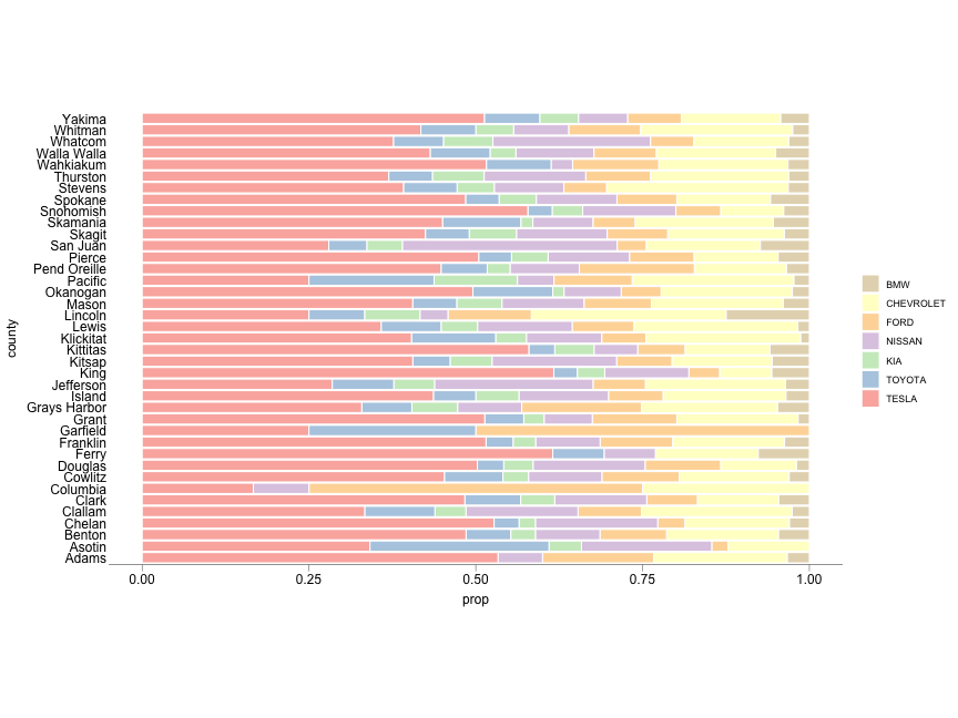<!-- --> ] --- count: false ## EV in WA state: Shares of makes across counties .panel1-make_share4-non_seq[ ```r ggplot(make_share_byCounty, aes(x = prop, y = county, fill = make)) + theme_cavis + geom_bar( position = "stack", stat = "identity", color = "white" ) + scale_fill_brewer( type = "qual", palette = 4 , direction = -1 ) + * scale_x_continuous( * expand = c(0, 0), * ) ``` ] .panel2-make_share4-non_seq[ 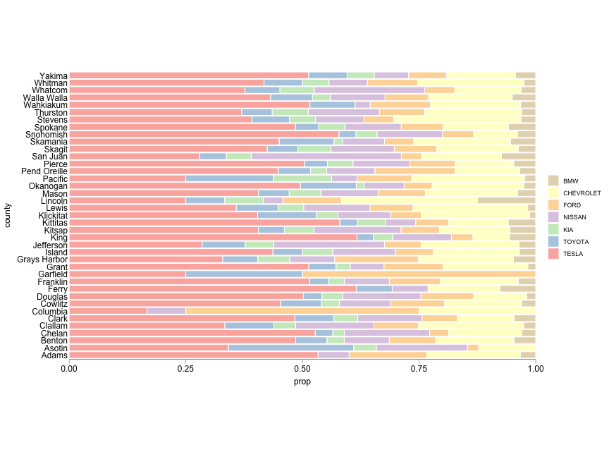<!-- --> ] --- count: false ## EV in WA state: Shares of makes across counties .panel1-make_share4-non_seq[ ```r ggplot(make_share_byCounty, aes(x = prop, y = county, fill = make)) + theme_cavis + geom_bar( position = "stack", stat = "identity", color = "white" ) + scale_fill_brewer( type = "qual", palette = 4 , direction = -1 ) + scale_x_continuous( expand = c(0, 0), * labels = label_percent(), * sec.axis = dup_axis() ) ``` ] .panel2-make_share4-non_seq[ 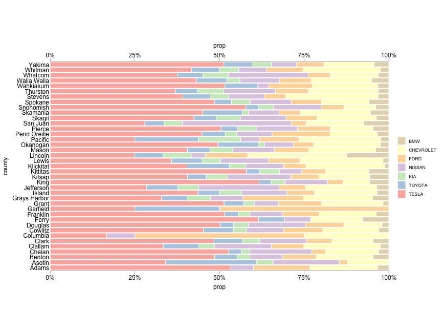<!-- --> ] --- count: false ## EV in WA state: Shares of makes across counties .panel1-make_share4-non_seq[ ```r ggplot(make_share_byCounty, aes(x = prop, y = county, fill = make)) + theme_cavis + geom_bar( position = "stack", stat = "identity", color = "white" ) + scale_fill_brewer( type = "qual", palette = 4 , direction = -1 ) + scale_x_continuous( expand = c(0, 0), labels = label_percent(), sec.axis = dup_axis() ) + * theme(aspect.ratio = 1.618) ``` ] .panel2-make_share4-non_seq[ 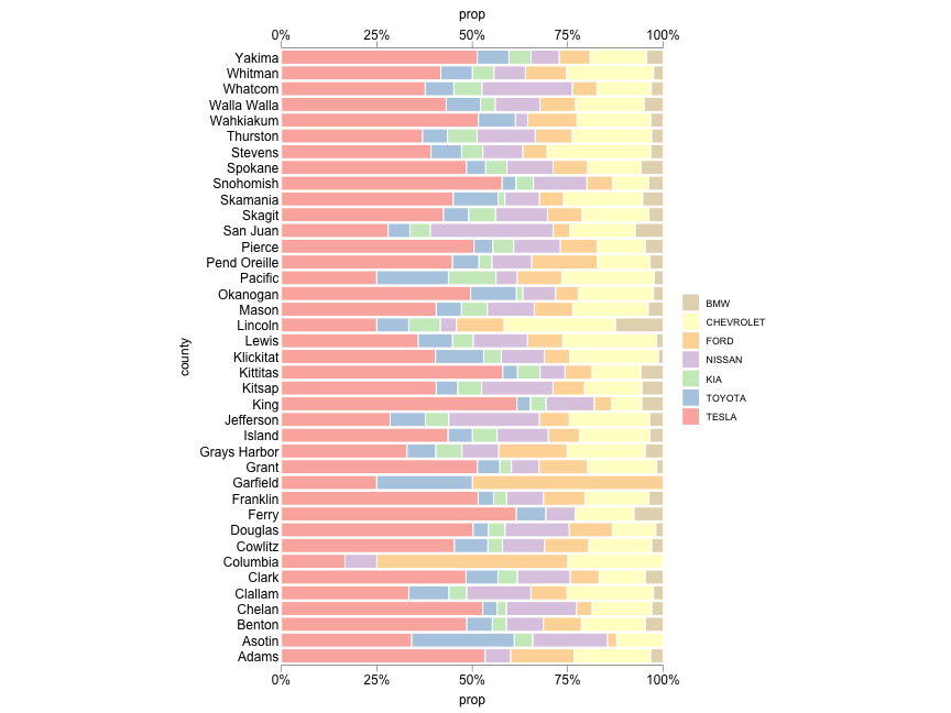<!-- --> ] --- count: false ## EV in WA state: Shares of makes across counties .panel1-make_share4-non_seq[ ```r ggplot(make_share_byCounty, aes(x = prop, y = county, fill = make)) + theme_cavis + geom_bar( position = "stack", stat = "identity", color = "white" ) + scale_fill_brewer( type = "qual", palette = 4 , direction = -1 ) + scale_x_continuous( expand = c(0, 0), labels = label_percent(), sec.axis = dup_axis() ) + theme(aspect.ratio = 1.618) + * labs(y = NULL, x = NULL) ``` ] .panel2-make_share4-non_seq[ 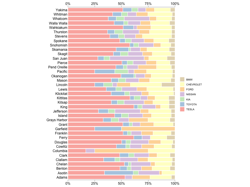<!-- --> ] <style> .panel1-make_share4-non_seq { color: black; width: 49%; hight: 32%; float: left; padding-left: 1%; font-size: 80% } .panel2-make_share4-non_seq { color: black; width: 49%; hight: 32%; float: left; padding-left: 1%; font-size: 80% } .panel3-make_share4-non_seq { color: black; width: NA%; hight: 33%; float: left; padding-left: 1%; font-size: 80% } </style> --- count: false ## EV in WA state: Shares of makes across counties .panel1-make_share5-user[ ```r *ggplot(make_share_byCounty, * aes(x = prop, * y = fct_reorder2(county, make, prop), * fill = make)) + * theme_cavis + * geom_bar( * position = "stack", stat = "identity", * color = "white" * ) + * scale_fill_brewer( * type = "qual", * palette = 4 , * direction = -1 * ) + * scale_x_continuous( * expand = c(0, 0), * labels = label_percent(), * sec.axis = dup_axis() * ) + * theme(aspect.ratio = 1.618) + * labs(y = NULL, x = NULL) ``` ] .panel2-make_share5-user[ 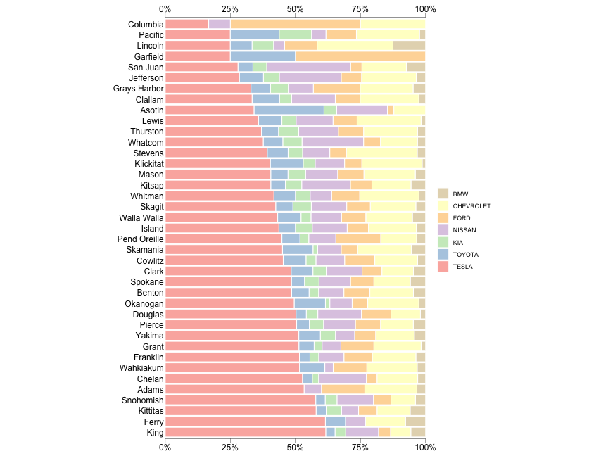<!-- --> ] --- count: false ## EV in WA state: Shares of makes across counties .panel1-make_share5-user[ ```r ggplot(make_share_byCounty, aes(x = prop, y = fct_reorder2(county, make, prop), fill = make)) + theme_cavis + geom_bar( position = "stack", stat = "identity", color = "white" ) + scale_fill_brewer( type = "qual", palette = 4 , direction = -1 ) + scale_x_continuous( expand = c(0, 0), labels = label_percent(), sec.axis = dup_axis() ) + theme(aspect.ratio = 1.618) + labs(y = NULL, x = NULL) ``` ] .panel2-make_share5-user[ <!-- --> ] <style> .panel1-make_share5-user { color: black; width: 49%; hight: 32%; float: left; padding-left: 1%; font-size: 80% } .panel2-make_share5-user { color: black; width: 49%; hight: 32%; float: left; padding-left: 1%; font-size: 80% } .panel3-make_share5-user { color: black; width: NA%; hight: 33%; float: left; padding-left: 1%; font-size: 80% } </style> --- count: false ## EV in WA state: Num. of EVs and median income .panel1-ev_income1-auto[ ```r *ev_data ``` ] .panel2-ev_income1-auto[ ``` # A tibble: 114,312 × 8 county city make model model_year ev_type electric_range retail_price <chr> <chr> <chr> <chr> <dbl> <chr> <dbl> <dbl> 1 Kittitas Cle Elum TESLA MODE… 2020 Batter… 291 0 2 Chelan Chelan TESLA MODE… 2020 Batter… 322 0 3 Snohomish Snohomi… TESLA MODE… 2018 Batter… 215 0 4 Thurston Tumwater FORD C-MAX 2014 Plug-i… 19 0 5 Kitsap Kingston FORD FUSI… 2013 Plug-i… 19 0 6 King Seattle NISS… LEAF 2018 Batter… 151 0 7 Skagit Mount V… AUDI E-TR… 2019 Batter… 204 0 8 Kitsap Port Or… NISS… LEAF 2019 Batter… 150 0 9 Snohomish Bothell TESLA MODE… 2020 Batter… 322 0 10 Yakima Tieton NISS… LEAF 2019 Batter… 150 0 # ℹ 114,302 more rows ``` ] --- count: false ## EV in WA state: Num. of EVs and median income .panel1-ev_income1-auto[ ```r ev_data %>% * group_by(county) ``` ] .panel2-ev_income1-auto[ ``` # A tibble: 114,312 × 8 # Groups: county [39] county city make model model_year ev_type electric_range retail_price <chr> <chr> <chr> <chr> <dbl> <chr> <dbl> <dbl> 1 Kittitas Cle Elum TESLA MODE… 2020 Batter… 291 0 2 Chelan Chelan TESLA MODE… 2020 Batter… 322 0 3 Snohomish Snohomi… TESLA MODE… 2018 Batter… 215 0 4 Thurston Tumwater FORD C-MAX 2014 Plug-i… 19 0 5 Kitsap Kingston FORD FUSI… 2013 Plug-i… 19 0 6 King Seattle NISS… LEAF 2018 Batter… 151 0 7 Skagit Mount V… AUDI E-TR… 2019 Batter… 204 0 8 Kitsap Port Or… NISS… LEAF 2019 Batter… 150 0 9 Snohomish Bothell TESLA MODE… 2020 Batter… 322 0 10 Yakima Tieton NISS… LEAF 2019 Batter… 150 0 # ℹ 114,302 more rows ``` ] --- count: false ## EV in WA state: Num. of EVs and median income .panel1-ev_income1-auto[ ```r ev_data %>% group_by(county) %>% * count() ``` ] .panel2-ev_income1-auto[ ``` # A tibble: 39 × 2 # Groups: county [39] county n <chr> <int> 1 Adams 35 2 Asotin 46 3 Benton 1394 4 Chelan 654 5 Clallam 741 6 Clark 6827 7 Columbia 13 8 Cowlitz 576 9 Douglas 227 10 Ferry 27 # ℹ 29 more rows ``` ] --- count: false ## EV in WA state: Num. of EVs and median income .panel1-ev_income1-auto[ ```r ev_data %>% group_by(county) %>% count() %>% * left_join(county_data, by = "county") ``` ] .panel2-ev_income1-auto[ ``` # A tibble: 39 × 4 # Groups: county [39] county n hh_num hh_income <chr> <int> <dbl> <dbl> 1 Adams 35 5720 40829 2 Asotin 46 9236 41665 3 Benton 1394 65304 57354 4 Chelan 654 27827 48674 5 Clallam 741 31329 44398 6 Clark 6827 158099 58262 7 Columbia 13 1762 43611 8 Cowlitz 576 40244 45877 9 Douglas 227 13894 48708 10 Ferry 27 3190 35485 # ℹ 29 more rows ``` ] --- count: false ## EV in WA state: Num. of EVs and median income .panel1-ev_income1-auto[ ```r ev_data %>% group_by(county) %>% count() %>% left_join(county_data, by = "county") %>% * mutate(n_EV_perhh = n / hh_num * 1000) ``` ] .panel2-ev_income1-auto[ ``` # A tibble: 39 × 5 # Groups: county [39] county n hh_num hh_income n_EV_perhh <chr> <int> <dbl> <dbl> <dbl> 1 Adams 35 5720 40829 6.12 2 Asotin 46 9236 41665 4.98 3 Benton 1394 65304 57354 21.3 4 Chelan 654 27827 48674 23.5 5 Clallam 741 31329 44398 23.7 6 Clark 6827 158099 58262 43.2 7 Columbia 13 1762 43611 7.38 8 Cowlitz 576 40244 45877 14.3 9 Douglas 227 13894 48708 16.3 10 Ferry 27 3190 35485 8.46 # ℹ 29 more rows ``` ] --- count: false ## EV in WA state: Num. of EVs and median income .panel1-ev_income1-auto[ ```r ev_data %>% group_by(county) %>% count() %>% left_join(county_data, by = "county") %>% mutate(n_EV_perhh = n / hh_num * 1000) -> * ev_by_income ``` ] .panel2-ev_income1-auto[ ] <style> .panel1-ev_income1-auto { color: black; width: 88.2%; hight: 32%; float: top; padding-left: 1%; font-size: 80% } .panel2-ev_income1-auto { color: black; width: 9.8%; hight: 32%; float: top; padding-left: 1%; font-size: 80% } .panel3-ev_income1-auto { color: black; width: NA%; hight: 33%; float: top; padding-left: 1%; font-size: 80% } </style> --- count: false ## EV in WA state: Num. of EVs and median income .panel1-ev_income2-auto[ ```r *ggplot(ev_by_income, * aes(x = hh_income, y = n_EV_perhh)) ``` ] .panel2-ev_income2-auto[ <!-- --> ] --- count: false ## EV in WA state: Num. of EVs and median income .panel1-ev_income2-auto[ ```r ggplot(ev_by_income, aes(x = hh_income, y = n_EV_perhh)) + * theme_cavis_hgrid ``` ] .panel2-ev_income2-auto[ <!-- --> ] --- count: false ## EV in WA state: Num. of EVs and median income .panel1-ev_income2-auto[ ```r ggplot(ev_by_income, aes(x = hh_income, y = n_EV_perhh)) + theme_cavis_hgrid + * geom_point(alpha = 0.75, color = blue) ``` ] .panel2-ev_income2-auto[ 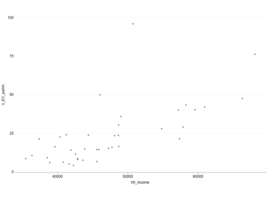<!-- --> ] --- count: false ## EV in WA state: Num. of EVs and median income .panel1-ev_income2-auto[ ```r ggplot(ev_by_income, aes(x = hh_income, y = n_EV_perhh)) + theme_cavis_hgrid + geom_point(alpha = 0.75, color = blue) + * scale_x_continuous(trans = "log10", * labels = label_dollar()) ``` ] .panel2-ev_income2-auto[ 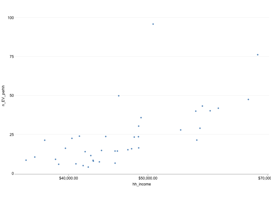<!-- --> ] --- count: false ## EV in WA state: Num. of EVs and median income .panel1-ev_income2-auto[ ```r ggplot(ev_by_income, aes(x = hh_income, y = n_EV_perhh)) + theme_cavis_hgrid + geom_point(alpha = 0.75, color = blue) + scale_x_continuous(trans = "log10", labels = label_dollar()) + * scale_y_continuous(trans = "log2") ``` ] .panel2-ev_income2-auto[ 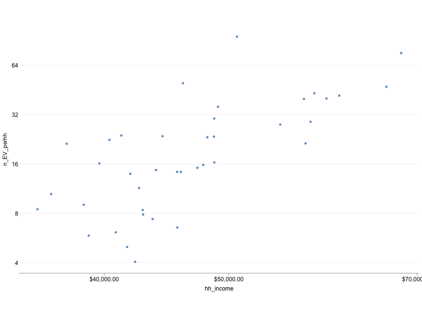<!-- --> ] --- count: false ## EV in WA state: Num. of EVs and median income .panel1-ev_income2-auto[ ```r ggplot(ev_by_income, aes(x = hh_income, y = n_EV_perhh)) + theme_cavis_hgrid + geom_point(alpha = 0.75, color = blue) + scale_x_continuous(trans = "log10", labels = label_dollar()) + scale_y_continuous(trans = "log2") + * geom_smooth(method = "lm", alpha = 0.2, * color = blue, fill = blue) ``` ] .panel2-ev_income2-auto[ 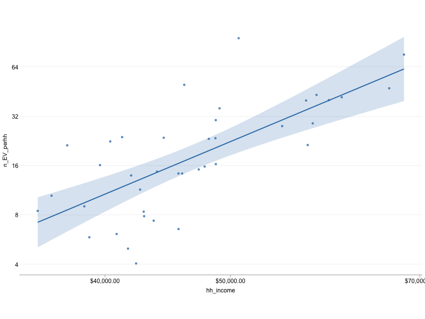<!-- --> ] --- count: false ## EV in WA state: Num. of EVs and median income .panel1-ev_income2-auto[ ```r ggplot(ev_by_income, aes(x = hh_income, y = n_EV_perhh)) + theme_cavis_hgrid + geom_point(alpha = 0.75, color = blue) + scale_x_continuous(trans = "log10", labels = label_dollar()) + scale_y_continuous(trans = "log2") + geom_smooth(method = "lm", alpha = 0.2, color = blue, fill = blue) + * labs(y = "N of EVs per 1,000 household", * x = "Median household income") ``` ] .panel2-ev_income2-auto[ 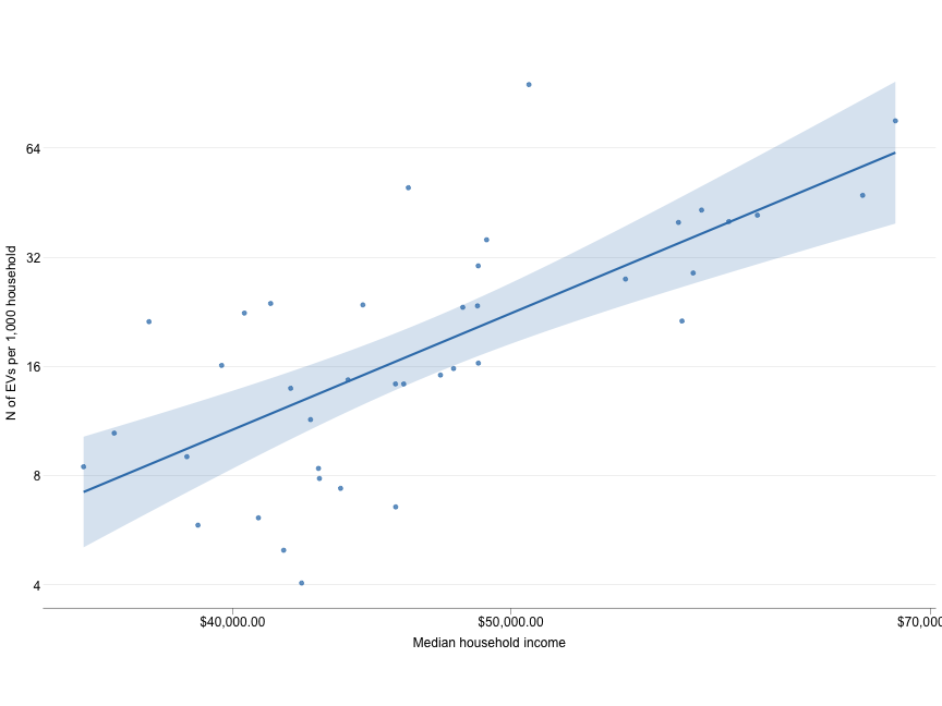<!-- --> ] --- count: false ## EV in WA state: Num. of EVs and median income .panel1-ev_income2-auto[ ```r ggplot(ev_by_income, aes(x = hh_income, y = n_EV_perhh)) + theme_cavis_hgrid + geom_point(alpha = 0.75, color = blue) + scale_x_continuous(trans = "log10", labels = label_dollar()) + scale_y_continuous(trans = "log2") + geom_smooth(method = "lm", alpha = 0.2, color = blue, fill = blue) + labs(y = "N of EVs per 1,000 household", x = "Median household income") + * geom_text_repel(aes(label = county)) ``` ] .panel2-ev_income2-auto[ 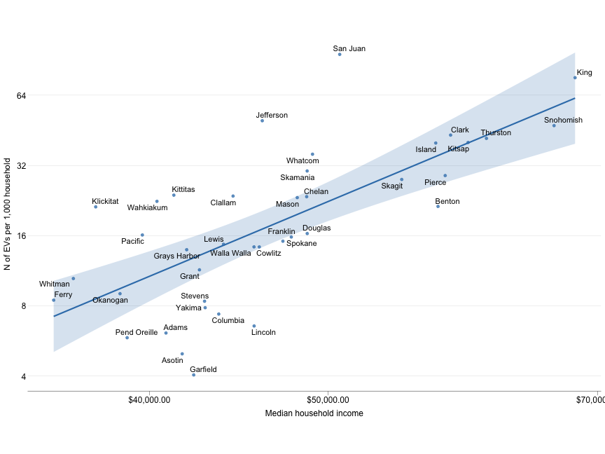<!-- --> ] <style> .panel1-ev_income2-auto { color: black; width: 49%; hight: 32%; float: left; padding-left: 1%; font-size: 80% } .panel2-ev_income2-auto { color: black; width: 49%; hight: 32%; float: left; padding-left: 1%; font-size: 80% } .panel3-ev_income2-auto { color: black; width: NA%; hight: 33%; float: left; padding-left: 1%; font-size: 80% } </style> --- count: false ## EV in WA state: Num. of EVs and median income .panel1-ev_income3-auto[ ```r # find outliners *lm(n_EV_perhh ~ hh_income, ev_by_income) ``` ] .panel2-ev_income3-auto[ ``` Call: lm(formula = n_EV_perhh ~ hh_income, data = ev_by_income) Coefficients: (Intercept) hh_income -52.683902 0.001614 ``` ] --- count: false ## EV in WA state: Num. of EVs and median income .panel1-ev_income3-auto[ ```r # find outliners lm(n_EV_perhh ~ hh_income, ev_by_income) %>% * broom::augment(ev_by_income) ``` ] .panel2-ev_income3-auto[ ``` # A tibble: 39 × 11 county n hh_num hh_income n_EV_perhh .fitted .resid .hat .sigma .cooksd <chr> <int> <dbl> <dbl> <dbl> <dbl> <dbl> <dbl> <dbl> <dbl> 1 Adams 35 5720 40829 6.12 13.2 -7.11 0.0426 14.8 5.51e-3 2 Asotin 46 9236 41665 4.98 14.6 -9.60 0.0385 14.7 9.01e-3 3 Benton 1394 65304 57354 21.3 39.9 -18.6 0.0653 14.5 6.04e-2 4 Chelan 654 27827 48674 23.5 25.9 -2.39 0.0263 14.8 3.73e-4 5 Clall… 741 31329 44398 23.7 19.0 4.66 0.0291 14.8 1.57e-3 6 Clark 6827 158099 58262 43.2 41.4 1.81 0.0728 14.8 6.48e-4 7 Colum… 13 1762 43611 7.38 17.7 -10.3 0.0312 14.7 8.35e-3 8 Cowli… 576 40244 45877 14.3 21.4 -7.07 0.0265 14.8 3.28e-3 9 Dougl… 227 13894 48708 16.3 26.0 -9.61 0.0264 14.7 6.03e-3 10 Ferry 27 3190 35485 8.46 4.60 3.86 0.0817 14.8 3.38e-3 # ℹ 29 more rows # ℹ 1 more variable: .std.resid <dbl> ``` ] --- count: false ## EV in WA state: Num. of EVs and median income .panel1-ev_income3-auto[ ```r # find outliners lm(n_EV_perhh ~ hh_income, ev_by_income) %>% broom::augment(ev_by_income) %>% * slice_max(order_by = abs(.resid), n = 10) ``` ] .panel2-ev_income3-auto[ ``` # A tibble: 10 × 11 county n hh_num hh_income n_EV_perhh .fitted .resid .hat .sigma .cooksd <chr> <int> <dbl> <dbl> <dbl> <dbl> <dbl> <dbl> <dbl> <dbl> 1 San J… 729 7613 50726 95.8 29.2 66.5 0.0301 9.61 0.333 2 Jeffe… 699 14049 46048 49.8 21.7 28.1 0.0263 14.0 0.0514 3 King 60059 789232 68065 76.1 57.2 18.9 0.196 14.4 0.254 4 Benton 1394 65304 57354 21.3 39.9 -18.6 0.0653 14.5 0.0604 5 Linco… 29 4422 45582 6.56 20.9 -14.3 0.0269 14.6 0.0137 6 Klick… 177 8327 37398 21.3 7.69 13.6 0.0651 14.6 0.0321 7 Pierce 8684 299918 57869 29.0 40.7 -11.8 0.0695 14.7 0.0261 8 Garfi… 4 989 42269 4.04 15.6 -11.5 0.0359 14.7 0.0120 9 Colum… 13 1762 43611 7.38 17.7 -10.3 0.0312 14.7 0.00835 10 Kitti… 396 16595 41232 23.9 13.9 9.98 0.0406 14.7 0.0103 # ℹ 1 more variable: .std.resid <dbl> ``` ] --- count: false ## EV in WA state: Num. of EVs and median income .panel1-ev_income3-auto[ ```r # find outliners lm(n_EV_perhh ~ hh_income, ev_by_income) %>% broom::augment(ev_by_income) %>% slice_max(order_by = abs(.resid), n = 10) %>% * pull(county) ``` ] .panel2-ev_income3-auto[ ``` [1] "San Juan" "Jefferson" "King" "Benton" "Lincoln" "Klickitat" [7] "Pierce" "Garfield" "Columbia" "Kittitas" ``` ] --- count: false ## EV in WA state: Num. of EVs and median income .panel1-ev_income3-auto[ ```r # find outliners lm(n_EV_perhh ~ hh_income, ev_by_income) %>% broom::augment(ev_by_income) %>% slice_max(order_by = abs(.resid), n = 10) %>% pull(county) -> * outliners ``` ] .panel2-ev_income3-auto[ ] <style> .panel1-ev_income3-auto { color: black; width: 88.2%; hight: 32%; float: top; padding-left: 1%; font-size: 80% } .panel2-ev_income3-auto { color: black; width: 9.8%; hight: 32%; float: top; padding-left: 1%; font-size: 80% } .panel3-ev_income3-auto { color: black; width: NA%; hight: 33%; float: top; padding-left: 1%; font-size: 80% } </style> --- count: false ## EV in WA state: Num. of EVs and median income .panel1-ev_income4-user[ ```r *ggplot(ev_by_income, * aes(x = hh_income, y = n_EV_perhh)) + * theme_cavis_hgrid + * geom_point(alpha = 0.75, color = blue) + * scale_x_continuous(trans = "log10", * labels = label_dollar()) + * scale_y_continuous(trans = "log2") + * geom_smooth(method = "lm", alpha = 0.2, * color = blue, fill = blue) + * labs(y = "N of EVs per 1,000 household", * x = "Median household income") ``` ] .panel2-ev_income4-user[ <!-- --> ] --- count: false ## EV in WA state: Num. of EVs and median income .panel1-ev_income4-user[ ```r ggplot(ev_by_income, aes(x = hh_income, y = n_EV_perhh)) + theme_cavis_hgrid + geom_point(alpha = 0.75, color = blue) + scale_x_continuous(trans = "log10", labels = label_dollar()) + scale_y_continuous(trans = "log2") + geom_smooth(method = "lm", alpha = 0.2, color = blue, fill = blue) + labs(y = "N of EVs per 1,000 household", x = "Median household income") + * geom_text_repel( * data = filter(ev_by_income, * county %in% outliners), * aes(label = county) * ) ``` ] .panel2-ev_income4-user[ 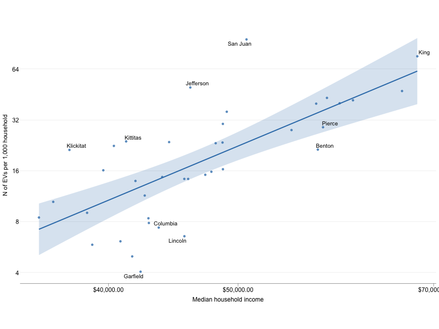<!-- --> ] <style> .panel1-ev_income4-user { color: black; width: 49%; hight: 32%; float: left; padding-left: 1%; font-size: 80% } .panel2-ev_income4-user { color: black; width: 49%; hight: 32%; float: left; padding-left: 1%; font-size: 80% } .panel3-ev_income4-user { color: black; width: NA%; hight: 33%; float: left; padding-left: 1%; font-size: 80% } </style> --- ## Some takeaways - Don't rely on defaults; starts with minimalist aesthetics -- - Understand the consequence of `inherit.aes = TRUE` and how to take advantage/overwrite it -- - Learn to scale everything (color, fill, x-axis, y-axis, etc) -- - Choose nice colors with `RColorBrewer` -- - Order things intelligently with `factor` -- - Save graphic output correctly with `ggsave`