0 2025/spectral-1031

Post by Agastya Ravuri (aravuri@andrew.cmu.edu)

Ideally, this post would be targeted at those who have just learned the basics of matrices and linear transformations in a first linalg class and are maybe just about to see the spectral theorem for symmetric matrices, or at someone who has seen the spectral theorem before but felt like they didn’t understand what it was really saying (me).

If my explanation of dual spaces/covectors ends up being too confusing, eigenchris’ Tensors for Beginners series is a great resource.

Finally got this done on the most spectral night of the year.

Motivation

Usually, when you hear someone state the spectral theorem, it’s something like the following: If I have a symmetric matrix, meaning it has the same values when reflected across its major diagonal (), then the following things hold:

1. It has eigenvalues (counting multiplicity)
2. It can be diagonalized by an orthogonal matrix (i.e, a rotation or a reflection); in other words, its eigenvectors are orthogonal.

When generalized to a complex matrix, we talk about a Hermitian (conjugate symmetric) matrix instead, meaning it has the same values when reflected across its major diagonals and all the values are complex conjugated (). Then,

1. It has eigenvalues (counting multiplicity), and they’re all real numbers.
2. It can be diagonalized by a unitary matrix (a matrix that preserves the complex dot product). In other words, its eigenvectors are “orthogonal.”

These turn out to be very useful statements: the spectral theorem is the reason why a multidimensional normal distribution will always have perpendicular major axes:

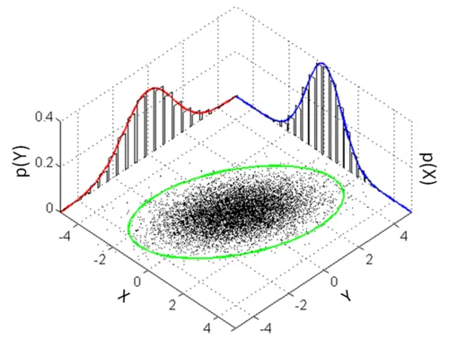
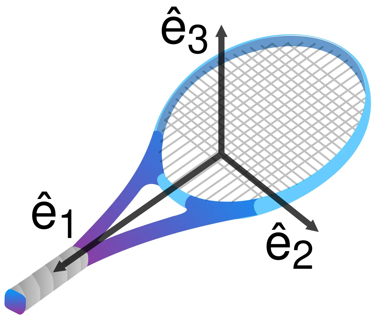
It’s the reason why all physical objects, no matter how weirdly shaped, will always have three perpendicular principal axes they rotate around.

It’s the reason why, for any (reasonable…) periodic function, I can write it as the sum of sine waves, and I can make that basis of waves orthonormal.

It’s the reason why all the quantum mechanical measurement operators have really nice properties, like how all their eigenstates are orthonormal (i think that one’s kinda reversed from the others because we defined it like that, but…).

With all these uses, the spectral theorem really starts to live up to its name: like a spectre, it influences many things we do from behind the scenes, and yet no mortal mind may comprehend what it means.

I would argue that the core of this confusion, at least for me, lay in the fact that I didn’t really know what a symmetric matrix was. To me, the spectral theorem said that this arbitrary class of matrices has an eigenbasis of orthogonal vectors. That’s a pretty cool property, but why would a matrix representing some linear transformation I randomly come across happen to be symmetric?

Overall, I want this post to bridge the gap between two intuitions for the spectral theorem, so keep these in mind:

1. The eigenvectors from the spectral theorem have something to do with maximization in a direction: For example, the principal axes of rotational inertia of an object are the directions with the maximum and minimum resistance, and the directions of these axes are the maximum and minimum covariance—can this be generalized?
2. The eigenvectors from the spectral theorem are orthogonal.

It turns out that both these properties are intimately related to the dot product, or, more generally, a dot product—as we’ll see, you can’t define “maximized in a direction” or “orthogonal” without it. This post seeks to give a deeper understanding of what a dot product is, and seeks to explain the “symmetric” property in that context. We will see how the spectral theorem is really a statement relating two dot products, and then present what is effectively the standard textbook proof of the spectral theorem except with this context in mind.

Note: this post will only talk about the spectral theorem for real symmetric matrices, which is its most used form; I assume there’s a similar argument for all normal matrices (the full class of unitarily diagonalizable matrices), but it’s probably more involved.

Dot Products

In 𝟚, the standard dot product is given by

but there are two problems with this definition.

First, this definition is basis-dependent, and we don’t really like that. If I was using a different basis of 𝟚, the dot product wouldn’t look like this. For example, if my basis was

then notice that

which doesn’t match up.

A lot of the time we find that it’s simpler to work in a weird basis, but the cost of this is that the dot product might not work how it normally does.

Second, the dot product is a way of encoding similarity between vectors: it’s positive when they’re aligned, 0 when they’re perpendicular, and negative when they are misaligned. However, we sometimes find that there are two different useful ways of thinking about similarity, and if you choose a basis where one of them is the standard dot product, the other looks completely screwed up.

Instead, then, we say that a dot product is a “positive-definite symmetric bilinear form.” Let’s go through what this means in reverse order, with representing the dot product:

1. Bilinear form: A function that takes in two vectors and returns a scalar and is linear in both arguments: and .
2. Symmetric: For all vectors , .
3. Positive-definite: For all , , and only if .

When looked at like a product, these properties correspond to the distributivity of multiplication, commutativity of multiplication, and trivial inequality respectively.

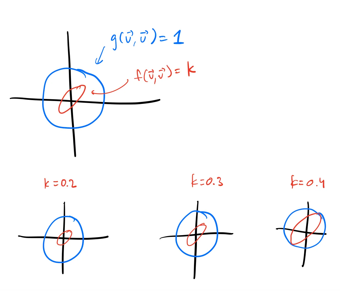
There are two concepts that we use the dot product for—magnitude and orthogonality. We can translate these ideas to any other dot product. The squared magnitude of a vector is , so we can generalize this and say that the -squared-magnitude of a vector is . Also we say that two vectors are orthogonal if , so we can say that vectors are -orthogonal if .

Geometrically, we can visualize it like this—the unit sphere of the regular dot product (the set of all points where ) is, of course, a sphere. In general, the unit sphere of an arbitrary dot product is some ellipsoid. If you don’t have the requirement of positive-definiteness, the unit “sphere” can instead be some other 3D conic section, like a hyperboloid.

Note: I’m going to be ignoring positive-definiteness for most of this post; it is important at one point (see if you can figure out where), but most of the time, feel free to think of the terms “dot product” and “symmetric bilinear form” interchangeably in this post.

Mathematically, a bilinear form is completely determined by where it sends pairs of basis vectors. As a result, as a matrix, we can represent them as a “row vector of a row vector”: for example, the standard dot product on can be represented as the following:

Why? Let’s see how we calculate . You can first apply it to a vector using regular matrix multiplication:

Then, you can apply that to , giving us a familiar formula.

In general, the th element of the th row vector of the matrix representation of a dot product , , represents , where and are the th and th standard basis vectors, respectively:

The symmetry property, then, means that for all , . In other words, the th element of the th row vector should be the same as the th element of the th row vector. This is suspiciously similar to the definition of a symmetric matrix .

Currying

This matrix representation is designed for multiplying with two vectors, but there’s nothing stopping us with multiplying with one vector at a time. In fact, notice what we did with the standard dot product earlier:

It converted the column vector into a row vector! In fact, for the standard dot product specifically, it returned the transpose of !

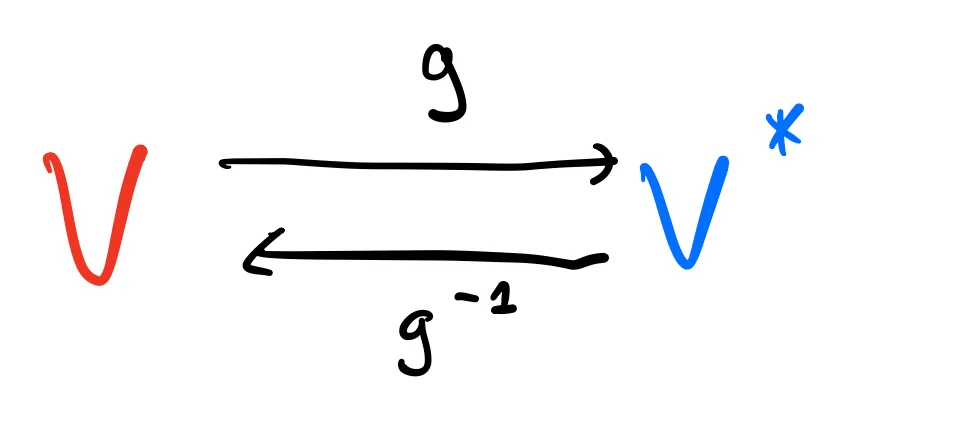
The dot product is usually viewed as a function , one that takes in two vectors and returns a real number. It’s sometimes useful to instead look at the curried dot product, , which is what we get when we apply the matrix once instead of twice. Basically, this is a function that takes in one vector, and then returns the single-variable function .

We call the space of all linear functions the dual space of , represented by . We call elements of that space covectors, row vectors, or matrices, which are terms that I’ll use pretty interchangeably in this post.

Geometrically, you can represent any covector as a set of parallel planes; then, to apply it to a vector, you count how many planes it crosses:

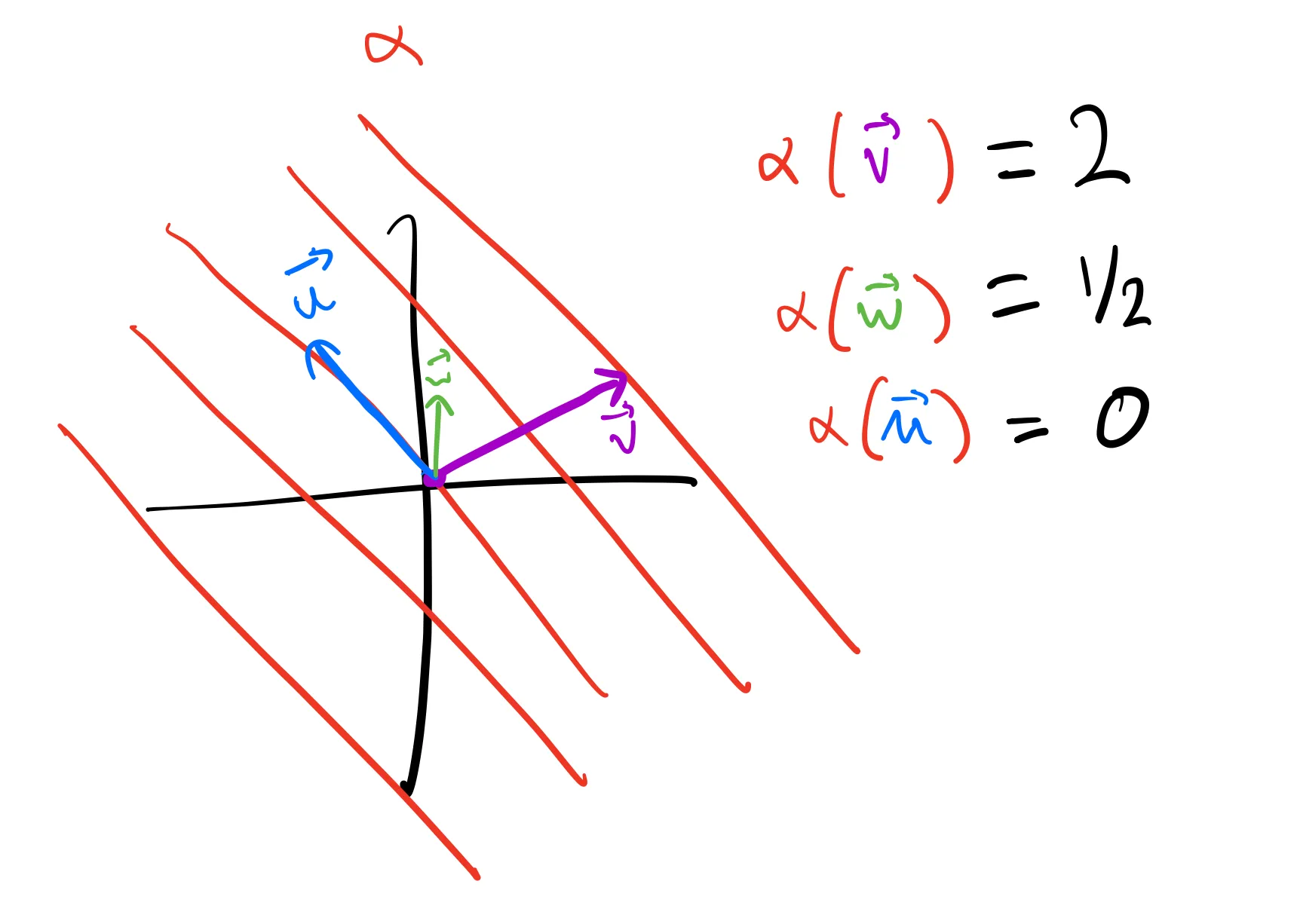
The kernel of a covector is the set of all vectors that it maps to zero. In this case, that’s represented by the plane through the origin.

As we’ve seen, a dot product is a transformation which takes in a vector and returns a covector. This transformation is actually invertible, which we can see with the standard dot product: for the standard dot product, will be the transpose of the column vector. This is clearly invertible, as if we take the transpose of the resulting row vector, we get back where we started.

Of course, for other dot products they won’t have such a nice representation, but in general, will convert a vector to a row vector and will convert a row vector to a vector:

Symmetric Matrices & Associated Linear Transformations

Now that we have talked about dot products, we can think about what happens if I have two of them. Let be dot products on . We know that a dot product is an isomorphism between a vector space and its dual space, so we can draw the following diagram:

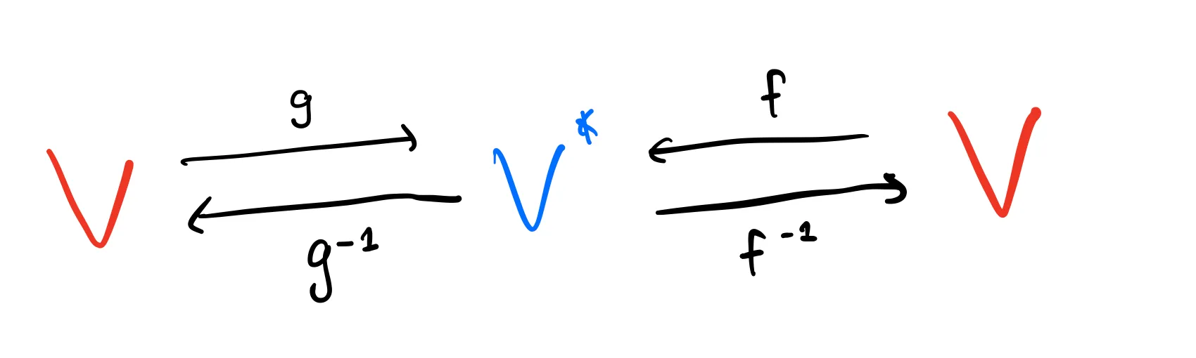
We can think of and as two different embeddings of the vector space into its dual space. Consider the map , which takes . This is just an automorphism on (in other words, a square matrix)! If we consider to be the standard dot product, we say that is ‘s “associated linear transformation (under )”. We call a matrix symmetric if it is the associated linear transformation of a symmetric bilinear form. Likewise, for a symmetric matrix, we say that its “associated symmetric bilinear form (under )” is .

You can think of this by looking at the bilinear form’s matrix representation. If is the standard dot product, and is some other dot product, represented by the matrix , recalling that the inverse dot product is the inverse transpose, can be represented as

We know that the symmetry property of dot products means that . We can finally see how the symmetry property of dot products relates to the symmetry property of matrices!

How do we think about this transformation geometrically? Well, consider that . The associated linear transformation, then, converts the -dot product into the -dot product. By symmetry of , this works for both arguments ().

For geometric intuition on what does, first, you apply to , giving you a row vector, or a linear function on ; the kernel of this row vector, , represents the set of all vectors that are -orthogonal to .

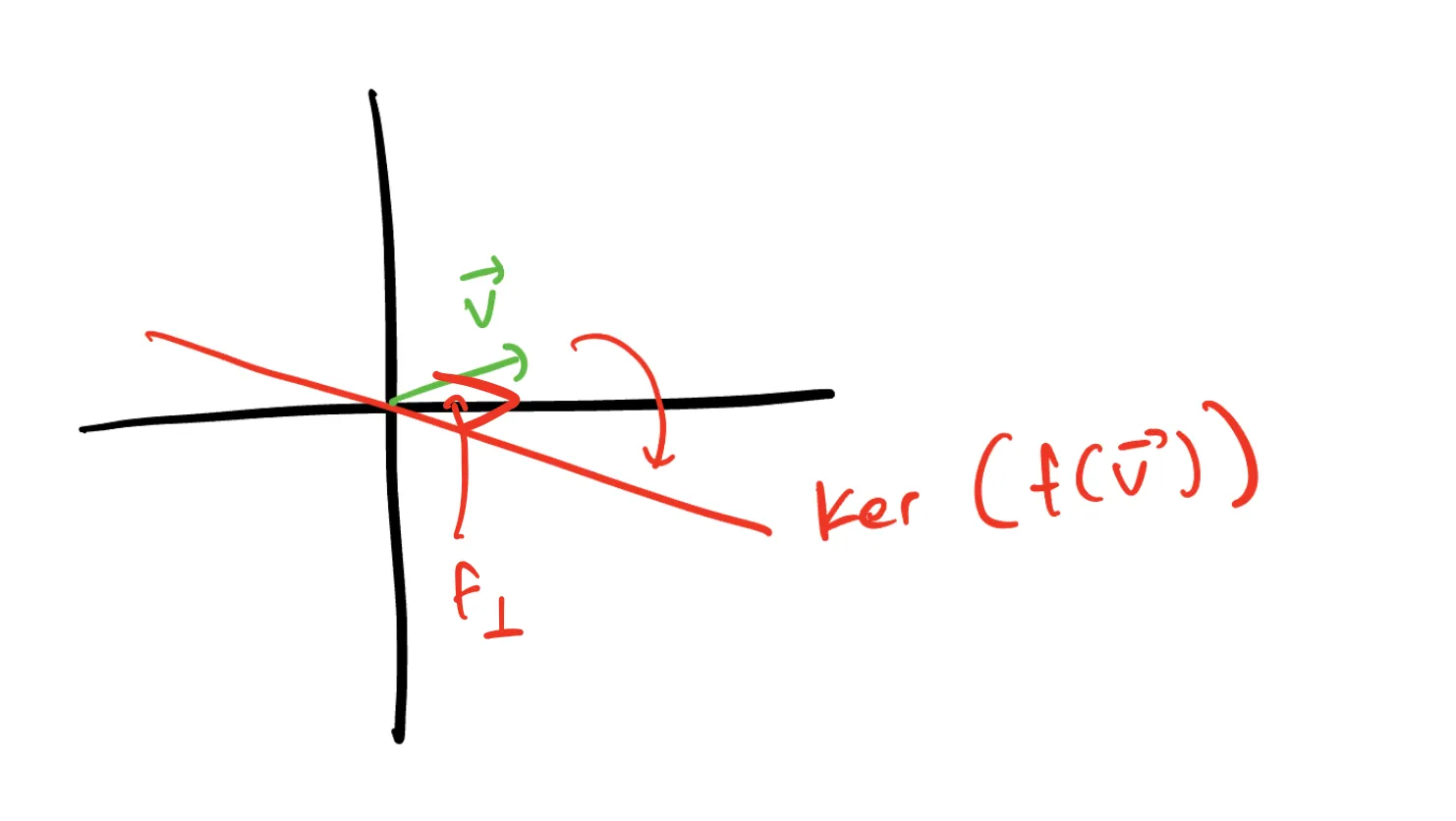
Then, when we apply to , we ask “give me a vector that is -orthogonal to this set.”

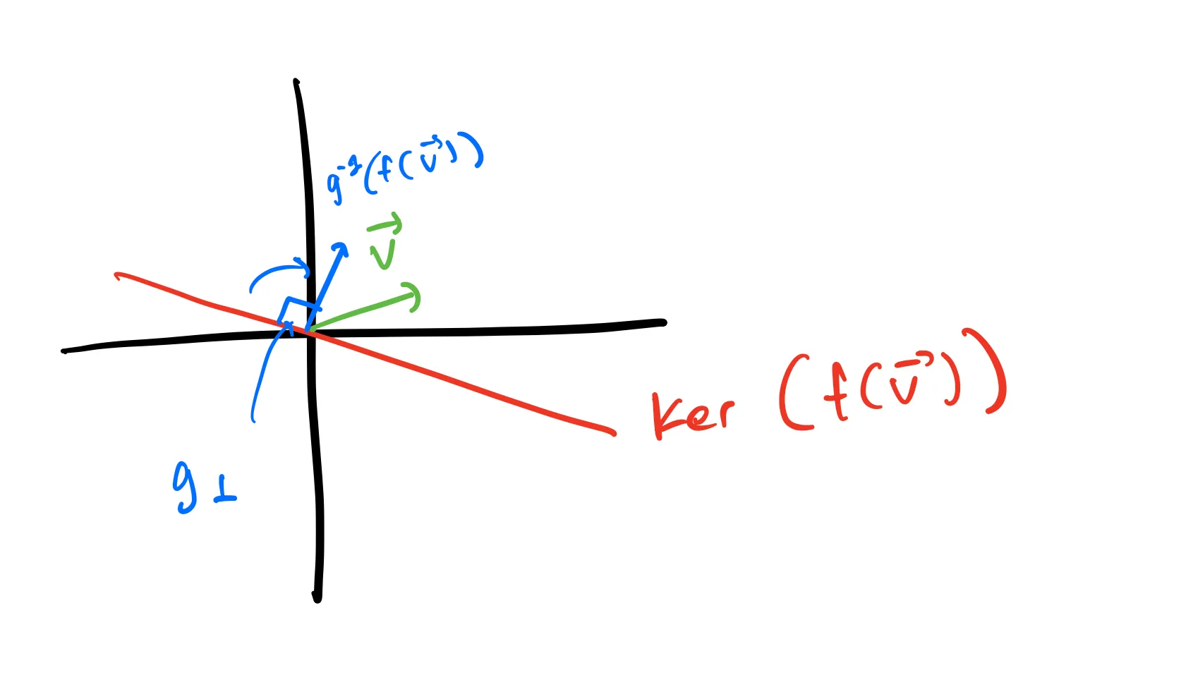
Therefore, we can think of as translating between two representations of the plane , the -embedding and the -embedding.

Note: will have a magnitude, dependent on the magnitude of the original and how and measure length, but it turns out we don’t have to think about it very much. In fact, if you think of vectors as simply their equivalence class under scalar multiplication (lines through the origin), that might help visually.

Eigenvectors

What does an eigenvector of represent? Unfolding the definition, we have that are an eigenvector-eigenvalue pair iff . Applying to both sides and using linearity, this is . If I have two covectors and one is a scaled version of the other, that means the same thing as them having the same kernel (think about how geometrically a covector is parallel planes). As a result, we can rewrite this as . In other words, is an eigenvector of if and only if and both agree on the space that is perpendicular to .

The standard statement of the spectral theorem is the following: Given a dot product and a symmetric matrix on , there exists a -orthogonal basis of such that is diagonal: each basis vector is an eigenvector.

If we write this in terms of , the associated bilinear form of , using our interpretation of eigenvector, this is the same thing as the following: There exists a basis that is both -orthogonal and -orthogonal on .

In my opinion, this is pretty nice characterization. It turns out that there’s a simple algorithm for constructing this basis, too, using the idea of maximization/minimization. Using this, we’re finally ready for the proof of the spectral theorem.

The Spectral Theorem

Consider the set of the vectors on the -sphere, defined by . For each of those vectors, consider how measures them, . By the extreme value theorem (spheres are compact), there is some vector on the -sphere for which is minimized. I claim that this vector is an eigenvector of , or equivalently .

The proof for this is pretty simple by using the idea of Lagrange multipliers. Imagine “blowing up” the -sphere, , starting from and slowly increasing it.

The minimum will be the first value of for which hits the sphere, and will be the point where it touches. At this point, is the plane tangent to the -sphere at , and is the plane tangent to the -sphere at . Clearly, the tangent spaces align at the extreme value (the principle of Lagrange multipliers), so . Therefore, is an eigenvector of .

Note: “Tangent space” actually doesn’t depend on a dot product. By definition, the tangent space of a norm are the directions for which that -length is locally stationary when going along them (); it turns out that this aligns with the definition of orthogonal (), which you can prove using calculus, the bilinearity property, and symmetry (note specifically how the last step hinges on symmetry!):

Ok, great! We’ve found one eigenvector of . How do we find the rest of them, and prove they’re all both and -orthogonal to ? Well, this also depends on the property of symmetry.

Consider the set . What is its image under ? Well, let be an arbitrary vector in that set. Because , by definition, , or are -orthogonal.

Now, what is ? We don’t know exactly, but by symmetry, we know , so must contain . From above, we know that first takes a vector to its -orthogonal plane, and then spits out a vector that is -orthogonal to that plane. Ok, but if is -orthogonal to the plane , and , then must surely be -orthogonal to . But this is just the defining property of being in !

What have we found? For any vector in , takes it to . But equals —therefore, we have found that , which used to be an automorphism , is also an automorphism (one dimension lower!).

Now, we’re basically done! If we repeat this process recursively, finding extreme values and then restricting to their orthogonal subspaces, we will end up with a basis of that is both and -orthogonal.

Symmetry in Real Life

This proof hinged on the fact that dot products being symmetric meant that orthogonality of vectors was a symmetric relation. I hope that makes it easier to imagine why matrices we see in nature might be symmetric—they encode some kind of symmetric relation.

I think it’s easiest to see this in the covariance case: If I have two random variables and , then if and only if and are independent. This should, pretty clearly, be symmetric: if and are independent, then surely and are too. As a result, the spectral theorem holds.

Moment of inertia is a little harder. There are two main formulas that involve the moment of inertia in physics (three, but the third is just the time derivative of the first): In two-dimensions, we can write and where those are all scalars (=angular momentum, =moment of inertia, angular velocity, =rotational kinetic energy). Generalizing to three dimensions, is some linear transformation where , and .

If we write the kinetic energy formula using our new funny dot product notation, , or, if we examine ‘s associated bilinear form , we have , and . Cool! Moment of inertia is just some 2-norm that “measures” angular velocity and spits out kinetic energy. All 2-norms can be naturally represented as a symmetric bilinear form, which is the unique bilinear form that agrees with the norm and has the property that “-orthogonal” aligns with the tangent space of , which is very useful (see the note from the spectral theorem proof above). Now all you have to ask is why moment of inertia is a 2-norm in the first place, which is a physics question that I don’t know the answer to (is it because doubling angular velocity doubles velocity of all the particles which quadruples kinetic energy? probably. why is energy proportional to velocity squared in the first place? God probably knows. I read this one post about how it comes from Galilean invariance). Anyway, this 2-norm idea is probably the most common reason that symmetric matrices show up in physics. For example, the stress tensor is symmetric. Why? It takes in strain and spits out the stress and is energy density, just as moment of inertia takes in angular velocity and spits out angular momentum and is energy. (i think. i don’t know much about continuum mechanics so don’t quote me on this one).

The Fourier transform is also kind of hard. It’s common knowledge that the waves from the Fourier transform are the eigenfunctions of the laplacian on , which is a circle, and all the waves happen to be orthogonal with respect to the inner product . Why is the laplacian (the second derivative) symmetric w.r.t. this dot product? Well, you can do the math and do integration by parts twice:

because a circle has no boundary so the term vanishes. So yeah, you can see that the bilinear form is in fact symmetric, but I have no intuition for why or what maximizing this means. I guess my best guess would be looking at that middle term in the above derivation? You’re basically doing the dot product on the derivative and maximizing that? What does that have to do with harmonics? If somebody who knows more reads this please help.

As for quantum mechanical operators being Hermitian… yeah sorry I can’t help you. I think that one mostly comes from asserting the Born rule?

Anyway, those are a couple examples of where the spectral theorem would show up. There are many more (the generalized second derivative test, spectral graph theory, etc.), but I hope this article and associated proof has given an intuition for why something might be symmetric and why the spectral theorem would apply to allow you to find extreme perpendicular values.

I’ll probably make a sequel about the SVD and how it generalizes the spectral theorem not just to square normal matrices but to all linear transformations between inner product spaces.

---

Log in to Comment

Firebase not Loaded

---