spherical harmonics

The spherical harmonics are the angular part of the solution to the hydrogenic wave equation; the modulus squared of the solution is interpretted as the probability. Part of the importance of the spherical harmonics is that they form a complete orthonormal set and can be used as a basis for expansions of functions in spherical coordinate system(for an example see multipole moments in complement Ex in Cohen-Tannoudji's volume 2 of Quantum Mechanics book). Clebsch-Gordon coefficients relate the spherical harmonics in different representations. In Mathematica program the spherical harmonics are implemented as SphericalHarmonicY[l,m,theta,phi]; in matlab they are not built in and will be defined as complex functions in SH.m and as real spherical harmonics squared in SH2.m In the spherical coordinate system the polar or colatitudinal angle varies as 0 to pi and the azimuthal or longitudinal coordinate varies from 0 to 2*pi. In matlab the angle instead of starting from the z axis and moving from 0 to pi starts from the xy plane. This makes for some confusion! By replacing all sin(theta) -> cos(theta) and cos(theta) -> sin(theta) everything works out with theta varying from -pi/2 to pi/2 instead of the polar angle varying from 0 to pi.

The representation of a complex function could be done by using different colors or by causing a rotation; the latter was chosen and rotation is represented by variation of light reflected off a rotating surface. Click the above button to start the animation of complex valued spherical harmonic amplitude. For m=0 the spherical harmonic is real and not rotating. Y(2,2) rotates twice as fast as Y(2,1). Y(1,-1) would rotate in the opposite direction to Y(1,1).

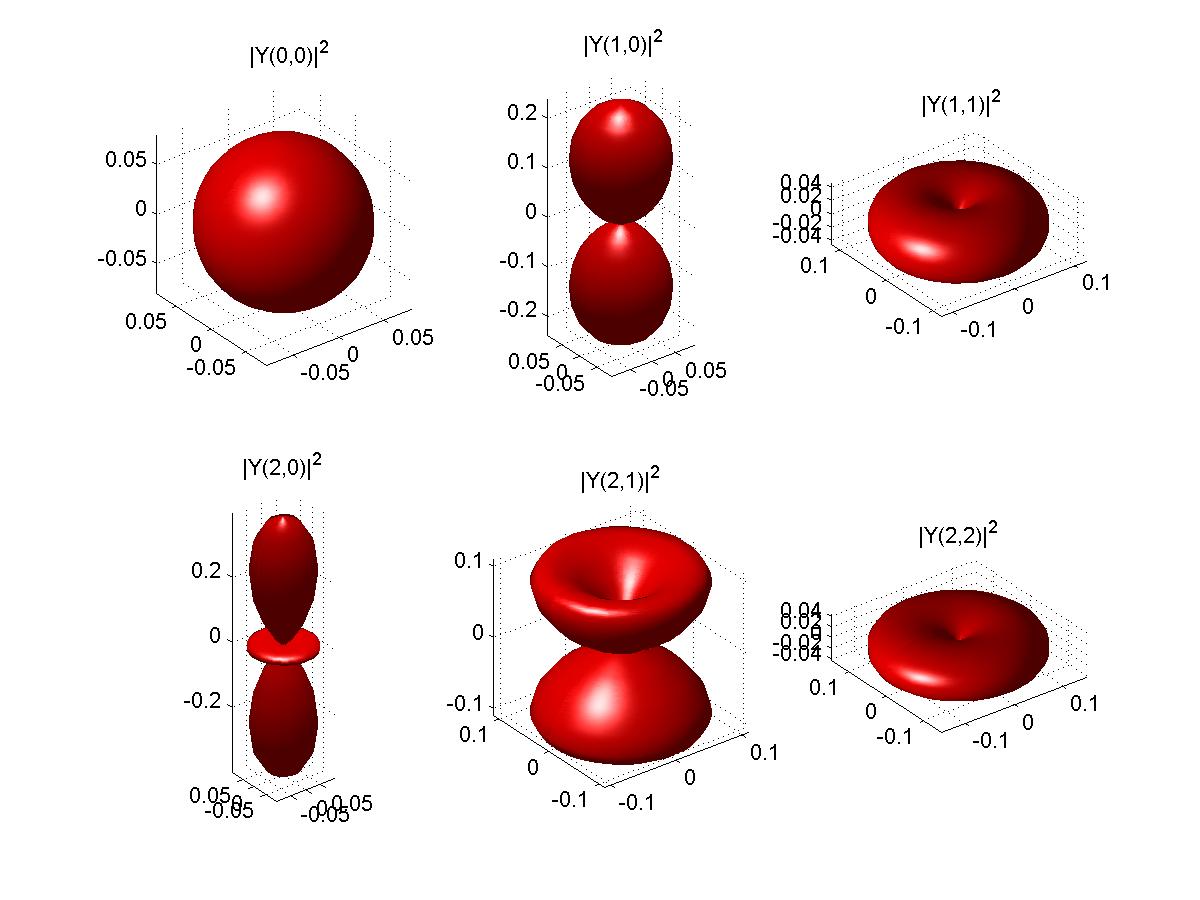
 The spherical harmonics squared are real and represented below:





 Many formulas
and some other plots ( not the same as the above complex functions)
of spherical harmonics are at 

http://mathworld.wolfram.com/SphericalHarmonic.html



Matlab program for sperical harmonic squared followed by
SH.m for complex spherical harmonic

%SHsquared.m
%Spherical Harmonics 
clear; clc;
%[X,Y]=meshgrid(-8:.5:8);
%R=sqrt(X.^2+Y.^2) + eps;
%Z=sin(R)./R;
%mesh(X,Y,Z,'EdgeColor','black')
%this was the sinc function

  THIS CODE IS DOWN FOR 
     REJUVENATION










title(' Y(1,0)');
axis equal;
%%%%%%%%%%%%%





























%mesh(X,Y,Z,'EdgeColor','black')


subplot(2,3,4);

camlight left; lighting phong

axis equal;


























%mesh(X,Y,Z,'EdgeColor','black')




camlight left; lighting phong
title('Y(2,2)');
axis equal;

%surf(X,Y,Z)
%colormap hsv
%colorbar
%surf(X,Y,Z)
%colormap hsv
%alpha(.4) 
% alpha ranges from 0(completely transparent to 1 (not transparent)

%surf(X,Y,Z,'FaceColor','red','EdgeColor','none')
%camlight left; lighting phong

%subplot(2,3,2);
%surfl(X,Y,Z)
%shading interp;
%colormap(pink);
%axis square;
%title('prob with Y(1,1)^2  / sin(theta)');









%this was the sinc function

















%surf(X,Y,Z,abs(sqrt(X*X+Y*Y)))


%surfl(X,Y,Z)
%shading interp;
%colormap(pink);

axis equal;
%%%%%%%%%%%%




  THE CODE IS DOWN FOR REJUVENATION












%%%%%%%%%%%%%





%mesh(X,Y,Z,'EdgeColor','black')










































surf(X,Y,Z,'FaceColor','red','EdgeColor','none')
camlight left; lighting phong

axis equal;

%%%%%%%%%%%%%%%%%%%%%%%%
%%%%%%%%%%%%%%%%%%%%%%%

THE CODE IS DOEN FOR REJUVENATION




%mesh(X,Y,Z,'EdgeColor','black')

%was shown
subplot(2,3,6);
surf(X,Y,Z,'FaceColor','red','EdgeColor','none')
camlight left; lighting phong











%surf(X,Y,Z,'FaceColor','red','EdgeColor','none')
%camlight left; lighting phong

%subplot(2,3,2);
%surfl(X,Y,Z)
%shading interp;
%colormap(pink);
%axis square;